| Issue |
A&A
Volume 706, February 2026
|
|
|---|---|---|
| Article Number | A197 | |
| Number of page(s) | 11 | |
| Section | The Sun and the Heliosphere | |
| DOI | https://doi.org/10.1051/0004-6361/202555230 | |
| Published online | 10 February 2026 | |
A solar jet-induced perturbation propagating through coronal loops and in-loop electron beam transport as indicated by type II and type N radio bursts
1
School of Space Science and Technology, Institute of Space Sciences, Shandong Key Laboratory of Space Environment and Exploration Technology, Shandong University Weihai Shandong 264209, PR China
2
Institute of Frontier and Interdisciplinary Science, Shandong University Qingdao Shandong 266237, PR China
3
Key Laboratory of Dark Matter and Space Astronomy, Purple Mountain Observatory, CAS Nanjing 210023, PR China
4
Yunnan Observatories, Chinese Academy of Sciences Kunming Yunnan 650216, PR China
★ Corresponding author: This email address is being protected from spambots. You need JavaScript enabled to view it.
Received:
21
April
2025
Accepted:
20
December
2025
Abstract
Aims. Solar type II radio bursts are commonly attributed to coronal shocks driven by coronal mass ejections (CMEs). However, some metric type II bursts have occasionally been reported to occur in the absence of a CME and to be associated with weak solar activity. The aim of this study is to identify the driver of the coronal shock in this kind of type II event.
Methods. We investigated a high-frequency metric type II burst with clear band splitting, observed simultaneously by the Chashan Broadband Solar radio spectrograph and the Nançay Radioheliograph. It is associated with a C3.1-class flare and a small-scale jet, but without a detectable CME in the coronagraphs.
Results. The type II burst is preceded by multiple type III bursts, one of which exhibits characteristics of a type N burst. The type II burst source is associated with the jet-induced perturbation front propagating through nearby closed loops at a speed of ∼880 km s−1, rather than the much slower jet front. This suggests that the disturbance initiated by the jet can convert to a shock wave within low Alfvénic coronal loops, providing the necessary conditions for electron acceleration and subsequent radio emission. Our findings offer new insights into the formation mechanism of high-frequency type II bursts associated with weak flares and jets.
Key words: Sun: activity / Sun: corona / Sun: flares / Sun: particle emission / Sun: radio radiation
© The Authors 2026
 Open Access article, published by EDP Sciences, under the terms of the Creative Commons Attribution License (https://creativecommons.org/licenses/by/4.0), which permits unrestricted use, distribution, and reproduction in any medium, provided the original work is properly cited.
This article is published in open access under the Subscribe to Open model. This email address is being protected from spambots. You need JavaScript enabled to view it. to support open access publication.
1. Introduction
Solar flares and coronal mass ejections (CMEs) are intense energy release activities in the solar atmosphere, capable of accelerating a large number of electrons to high energies. These energetic electrons further generate various types of radio bursts through coherent radiation mechanisms, such as plasma emission (Ginzburg & Zhelezniakov 1958; Pick & Vilmer 2008). Solar radio bursts at decimeter–meter wavelengths serve as one of the primary diagnostics for the acceleration and transport of energetic electrons in the corona.
Type II and type III radio bursts are the most commonly observed radio emissions associated with explosive solar activities. Type II bursts appear as narrow bands that slowly drift in radio dynamic spectra and are attributed to energetic electrons accelerated at outward-propagating shock fronts (Nelson & Melrose 1985). Most type II bursts exhibit intermittent or patchy emission bands. In many events, the fundamental and harmonic bands of type II bursts can further split into sub-bands, known as the band splitting phenomenon (e.g., Smerd et al. 1975; Vršnak et al. 2001; Du et al. 2014, 2015). In addition to the main emission lanes, various fine structures are often observed, including herringbones, characterized by short-duration drifts toward low and high frequencies from a type II burst backbone (Holman & Pesses 1983). In contrast, type III bursts drift much more rapidly in radio dynamic spectra, representing the propagation of fast electron beams (∼0.1−0.3c, where c is the speed of light) accelerated through magnetic reconnection during solar flares and propagating along open or large-scale closed magnetic field lines (Reid 2020). The solar corona is pervaded by closed magnetic loops. When electron beams propagate along a coronal loop, the frequency drift reverses as they pass the loop top and turn toward the Sun, resulting in type III burst variants, including type J and type U bursts (e.g., Reid & Kontar 2017; Mancuso et al. 2023; Feng et al. 2024). If the electron beams encounter reflection due to the magnetic mirroring effect of coronal loops, a type N burst can be observed (e.g., Caroubalos et al. 1987; Kong et al. 2016).
Metric type II bursts and their fine structures are generally identified as radio signatures of CME-driven shocks through the solar corona (e.g., Zimovets et al. 2012; Feng et al. 2016; Lv et al. 2017; Morosan et al. 2019; Kouloumvakos et al. 2021; Koval et al. 2024). However, not all type II radio bursts correlate with CME-driven shocks (e.g., Nindos et al. 2011; Magdalenić et al. 2012; Su et al. 2015; Kumari et al. 2023; Vasanth 2024). Different physical mechanisms have been proposed to explain the driver of type II bursts in the absence of associated CMEs. Su et al. (2015) suggested that when the strongly inclined magnetic loops reconnected with the newly emerging flux near the active region (AR), the fast expansion of the loops driven by magnetic tension forces could generate coronal shock waves that accelerated energetic electrons to produce type II bursts. Kumar et al. (2016) established that the high-frequency type II burst was associated with an extreme-ultraviolet (EUV) wave triggered by magnetic reconnection during the flare, and that the wave later evolved into a fast shock as it propagated through nearby loops. Specifically, some type II events have been found to be accompanied by only C-class flares and narrow jets (e.g., Maguire et al. 2021; Duan et al. 2022; Hou et al. 2023; Morosan et al. 2023). Maguire et al. (2021) showed that the type II burst source observed by LOw-Frequency ARray (LOFAR) was located much higher than the jet and propagated much faster. Therefore, they suggested that the narrow jet could produce a piston-driven shock ahead of it. For another event, Morosan et al. (2023) found that the type II burst source was ahead of jet-disturbed loops and proposed that the EUV wave may steepen into a shock wave in surrounding regions with low Alfvén speeds.
Recently, a high-performance solar radio spectrograph at meter wavelengths was developed at the Chashan solar radio observatory (CSO). More than 50 type II bursts have been recorded since its operation began1. For this paper we selected an event that occurred on 2023 May 8 without accompanying CMEs and that was associated with a C-class flare and coronal jet. We investigated the origin of the type II burst by combining multi-wavelength observations. The paper is organized as follows. We describe the observations in Section 2 and present the results of our analysis in Section 3. The summary and discussion are given in Section 4.
2. Observations
The radio burst event that occurred on 2023 May 8 was identified with radio spectral data from the Chashan Broadband Solar radio spectrograph at meter wavelengths (CBSm; Chang et al. 2024). CBSm is located at the CSO and is managed by the Institute of Space Science of Shandong University. It is designed to monitor high-frequency solar radio bursts at metric wavelengths. Its frequency range is 90−600 MHz, with a frequency resolution of about 76.294 kHz and a high temporal resolution of up to 0.21 ms. Since the start of its operation in November 2022, more than 50 type II radio bursts have been recorded.
Simultaneously, the Nançay Radioheliograph (NRH; Kerdraon & Delouis 1997) has provided radio imaging at ten different frequencies from 150 to 445 MHz for this radio burst event, with a 3-dB bandwidth of 700 kHz. Here we focus on analyzing the NRH data at three frequencies: 150, 173, and 228 MHz. The spatial resolution of the NRH is determined by its half-power beam width, calculated using the NRH routine in the SolarSoftWare. During the event, the half-power beam size at 150 MHz was 489.6″ (major axis of beam ellipse) and 264.4″ (minor axis of beam ellipse), at 173 MHz it was 420.2″ and 236.6″, and at 228 MHz it was 322.1″ and 172.9″, respectively. Due to the early morning observation, the low solar elevation angle resulted in beam elongation. However, since we focus on the variation of the centroids of radio sources, this effect can be negligible. Additionally, because NRH radio sources are observed at high frequencies and in the harmonic band, and the event occurred near the solar disk center, positional shifts arising from anisotropic scattering can be neglected for this event (e.g., Kontar et al. 2019; Chen et al. 2020; Kontar et al. 2023).
We examined the coronagraph images in the duration of the type II radio burst, taken by the Large Angle Spectrographic Coronagraph (LASCO; Brueckner et al. 1995) C2 on board the Solar and Heliospheric Observatory (SOHO) and the Sun Earth Connection Coronal and Heliospheric Investigation (SECCHI; Howard et al. 2008) on board the Solar Terrestrial Relations Observatory (STEREO), but no signatures of CMEs could be observed. The only eruptive feature is the onset of a C3.1-class flare accompanied by a small-scale jet from the NOAA AR 13296 (N13W12). The eruption was observed by multiple instruments, including the Atmospheric Imaging Assembly (AIA; Lemen et al. 2012) on board the Solar Dynamics Observatory (SDO; Pesnell et al. 2012). The EUV data from AIA were primarily used to analyze the flare and jet in this study. The Hard X-ray Imager (HXI; Su et al. 2019) payload of the Advanced Space-Based Solar Observatory (ASO-S; Gan et al. 2019) was employed to observe the nonthermal hard X-ray (HXR) emission of the solar flare. HXI covers an energy range of ∼10−300 keV for spectroscopy and ∼15−300 keV for imaging, with a maximum operational temporal cadence of 0.25 s and a spatial resolution of 3.1″ (Su et al. 2024). Meanwhile, the Gamma-ray Burst Monitor (GBM; Meegan et al. 2009) on the Fermi satellite provides count rates in the range of 8 keV to 1 MeV.
3. Results
A weak C3.1-class flare occurred simultaneously with the type II radio burst, as observed in the GOES soft X-ray (SXR) light curve in Figure 1a. The flare began at 08:20:00 UT, peaked at 08:25:00 UT, and ended at 08:49:24 UT. Figure 1b shows a composite of radio dynamic spectra from CSO/CBSm, Learmonth, and GERMANY-DLR in the range 50−300 MHz from 08:22:00 UT to 08:28:00 UT. Various types of radio bursts, including type III-like (J, N), type III, and type II bursts, were recorded. During the early impulsive phase of the flare between 08:22:00 and 08:23:24 UT, when the SXR flux began to rise, type III and type III-like radio bursts were already generated, indicating that electrons accelerated by magnetic reconnection had propagated outward along magnetic field lines of different configurations. This resulted in distinct frequency-drift patterns and intensities on the radio spectrogram. A type N burst, resembling the letter N (Kong et al. 2016), occurred before 08:23:00 UT, with other type III bursts around. An intense period of type III bursts manifested later during the flare impulsive phase between 08:23:30−08:24:18 UT, approximately coincident with the peak in the HXR flux. They drifted continuously to low frequencies (an interplanetary type III burst observed by STEREO-A/WAVES). The type II burst occurred at 08:26:30 UT after the flare SXR peak time during the gradual phase. It exhibits both fundamental (F) and harmonic (H) lanes, with clear band-spitting in the harmonic emission.
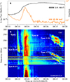 |
Fig. 1. Overview of the event on 2023 May 8. (a) GOES 1−8 Å soft X-ray light curve (black) of the C3.1-class flare and the ASO−S/HXI count rate from combined total flux detectors (D92+D93+D94) in the 25−50 keV energy channel (orange) between 08:22 and 08:28 UT. (b) Radio dynamic spectrum observed by CSO/CBSm (110−300 MHz), Learmonth (80−110 MHz), and GERMANY-DLR (50−80 MHz), displaying various type III and type III-like (J, N) bursts followed by a type II burst. Both fundamental (F) and harmonic (H) emission lanes can be identified for the type N burst and type II burst. |
3.1. Flare and jet eruption
The characteristics of the flare and jet in the eruptive AR are shown in Figure 2. Panels a1–a4, b1–b4, and c1–c4 are a sequence of EUV images in the AIA 131 Å, 171 Å, and 304 Å channels, respectively, presenting an overview of the eruption process in AR 13296 near the solar disk center. As shown in Figure 2c1, the AR was located near a magnetic polarity inversion zone, with two clearly visible mini-filaments (F1, F2) in 304 Å. During the early phase of the eruption (08:20:05−08:23:09 UT), no clear filament rise can be observed, possibly due to the high altitude of the filaments and intense flare brightening. At 08:23:09 UT, a jet is observed on the southern side of the AR, followed by the ejection of dark filament material with likely untwisting motion (see online animation). After the jet eruption, the mini-filaments disappeared (Fig. 2c4).
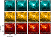 |
Fig. 2. EUV images in the AIA 131 Å, 171 Å, and 304 Å wavelengths (from top to bottom), showing the circular-ribbon flare and jet eruption. The white and black contours in panel c1 respectively represent the positive and negative magnetic fields of the HMI LOS magnetogram scaled at ±120 G. In panel c3 the green and blue curves mark the locations of filaments F1 and F2, respectively, as observed in panel c1. (The associated movie is available online). |
Figures 3a–c present a series of GONG Hα images before, during, and after the jet eruption, respectively. The two filaments F1 and F2 can be identified from the GONG Hα data before the eruption. However, filament F1 appears to be indistinct as a result of the lower spatial resolution of GONG. The filament structures finally disappeared after the eruption, as shown in Figure 3c, consistent with the observation in AIA 304 Å.
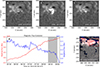 |
Fig. 3. (a)–(c) GONG Hα images before, during, and after the jet eruption. The white arrows in panel a indicate the two mini-filaments. (d) Evolution of the positive (red) and negative (blue) magnetic flux between 05:20 and 09:10 UT. The gray shaded region indicates the period of the flare. (e) HMI vector magnetic field map at 08:24:00 UT. The red and blue arrows represent the transverse field for positive and negative polarities, respectively. The length of the arrows indicates the magnetic field strength and the direction corresponds to the azimuthal orientation. |
To investigate the trigger mechanism of the filament eruption, we further analyzed the observation characteristics of magnetic flux and vector magnetic field in the AR. Figure 3d shows the temporal evolution of the magnetic flux near the polarity inversion line (PIL). It is calculated from the HMI LOS magnetograms for the target region, marked by the red rectangle in Figure 3e, over a time range from three hours before the eruption to 10 minutes after the flare (05:20−09:10 UT). The negative magnetic flux exhibits a significant and continuous decrease, while the positive magnetic flux shows a sustained increase due to the movement of positive polarity into the target region, suggesting that magnetic cancellation was ongoing during the flare (08:20−09:00 UT, shaded region in Figure 3d). Therefore, magnetic cancellation may be a key triggering factor in the eruption of mini-filaments. This finding is consistent with the widely observed physical mechanism in quiet-regions and coronal hole jets, where small-scale filament eruptions are triggered by magnetic flux cancellation (e.g., Adams et al. 2014; Sterling et al. 2015; Panesar et al. 2016; McGlasson et al. 2019).
Based on the HMI vector magnetograms with a 12-minute cadence, we also analyzed the tranverse magnetic field evolution in the AR. As shown in Figure 3e, significant magnetic shear motion is observed near the PIL, where the transverse magnetic field arrows of the positive and negative polarity regions are nearly parallel. Magnetic cancellation and shear cause the opposite polarity magnetic fields to continuously approach each other at the neutral line, triggering magnetic reconnection that alters the magnetic configuration. During this process, the erupting magnetic structure drives both internal and external reconnection: internal reconnection releases significant flare energy, manifesting as a C3.1-class flare with circular ribbons, while external reconnection, driven by the eruption of mini-filaments, opens magnetic field lines to produce the jet (e.g., Adams et al. 2014; Sterling et al. 2015; Panesar et al. 2016).
Energetic electrons accelerated during magnetic reconnection in the jet eruption produced nonthermal HXR emission. Figure 4a shows that the ASO-S/HXI light curves in the energy range of 15−300 keV began to rise around 08:23:00 UT. The flux curves from Fermi/GBM in the energy range of 4−300 keV have the same rising trend as the HXI light curves (Fig. 4b). Both reach their peaks at 08:23:52 UT, as marked by the vertical red dashed lines. The weak GBM signals above 100 keV may originate from the emission of electrons with energies exceeding 100 keV, indicating possible electron acceleration up to ∼100 keV in this weak C-class flare. The HXI exhibits no signal above 100 keV, primarily due to its detector area being over ten times smaller than that of the GBM and to its higher background signals.
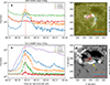 |
Fig. 4. HXR light curves and imaging of the flare in the duration of radio bursts. (a) ASO-S/HXI count rates of combined total flux detectors (D92+D93+D94) in three energy channels in the range 15−300 keV. (b) Fermi/GBM HXR flux in five channels in the range 4−300 keV. The red dashed lines indicate the peak of the curves at 08:23:52 UT. (c) and (d) Contours of HXR sources from HXI, in energy ranges of 15−25 keV (orange), 20−30 keV (blue), and 30−50 keV (red), overplotted on the AIA 1600 Å and HMI magnetogram images. The contour levels represent 25% and 60% of the maximum. The yellow arrow indicates the positive polarity at the center of the circular ribbon. |
For this flare event, the HXI is able to provide reliable imaging of HXR sources during the impulsive phase of the flare. HXR sources are reconstructed using the background-subtracted counts of HXI detectors from D19 to D91 (which are well calibrated), integrating from 08:23:56 UT to 08:24:24 UT, by the HXI_Clean algorithm (Su et al. 2024). The locations of HXR sources of different energies (in Fig. 4c) are cospatial with the circular ribbons in the AIA 1600 Å image, suggesting that the HXR emission is mainly produced at the footpoints of newly reconnected field lines due to the collision of energetic electrons with the low atmosphere. As indicated by the arrow in Figure 4d, the magnetic polarity in the center of the circular ribbon is positive and surrounded by negative polarities, consistent with the fan-spine topology (e.g., Zhong et al. 2019; Duan et al. 2022, 2024; Zhang et al. 2022; Zhang 2024). Additionally, as shown in Figure 2, the shape of the jet as it develops also supports the presence of a fan-spine magnetic configuration in the AR. Both the flare ribbon and HXR sources are located near the polarity inversion region. As shown in Figure 3 and discussed above, magnetic flux emergence and shear motion create preferred sites for magnetic reconnection and electron acceleration in the complex magnetic fields during the jet eruption (e.g., Glesener et al. 2012; Chen et al. 2018).
3.2. Type N radio burst
As shown in Figure 1b, during the impulsive phase of the flare (before 08:25 UT), multiple episodes of fast-drifting type III and type III-like bursts can be observed, indicating accelerated electron beams propagating outward along open or large-scale closed magnetic field lines. Specifically, the most intense type III burst occurred simultaneously with the HXR peak time. This demonstrates that the electrons generate HXR and radio emissions may have the same origin. Here we focus on the likely type N burst in the early impulsive phase. It appeared before 08:23 UT, when the HXR flux in low-energy channels of Fermi/GBM exhibited a rise. We note that unlike its harmonic counterpart, the fundamental emission of this type N burst is relatively weak and does not exhibit the complete N-shaped profile, consistent with the event investigated in our previous work (Kong et al. 2016). This may be attributed to the fact that the fundamental emission is subject to relatively strong scattering effects (Kontar et al. 2019).
Figure 5a presents a zoomed-in view of the radio dynamic spectrum from CSO/CBSm with a temporal resolution of 0.1 s, highlighting the harmonic emission of the type N burst. We note that the scale of the frequency-axis is reversed for easier comparison with the schematic diagram illustrating the generation of a type N burst, as shown in Figure 5b. The emission lanes of the type N burst are illustrated by the black dashed curve, which consists of three branches. The frequency drift rate is approximately −44 MHz s−1 from 228 to 150 MHz for the first branch, and 15 MHz s−1 from 150 to 173 MHz for the second branch. Caroubalos et al. (1987) revealed a smaller frequency drift rate for the second branch from the analysis of 16 “true” type N bursts, and they explained this phenomenon by the geometrical propagation effect, as the electron beam associated with the second branch is directed toward the Sun. Other contributing factors include the asymmetry or inclination of coronal loops, energy loss and pitch-angle scattering due to Coulomb collisions, and continuous variation in parallel velocity due to the magnetic mirror effect. We note that the drift rate for the first branch is generally consistent with previous statistical results for type III bursts (e.g., Zhang et al. 2018), indicating the average speed being ∼0.2c. In addition, we can see the duration of emission lanes basically increases for the three successive branches; the third branch is the most diffuse, which is likely due to the dispersion of the same electron beam along its path. The brightest emission is during the transition between the first and second branches (at the loop top) and the emission generally fades out between the second and third branches (around the mirror point). The above observational properties are generally consistent with those of type N bursts reported in previous studies (Caroubalos et al. 1987; Kong et al. 2016).
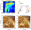 |
Fig. 5. Radio spectral and imaging observations of the type N burst (harmonic emission). (a) CSO/CBSm radio spectrum, the type N burst is outlined by the black dashed curve. The white dashed lines indicate the three NRH imaging frequencies at 150, 173, and 228 MHz. The red symbols mark the six selected data points shown in panels c and d. (b) Schematic diagram illustrating the generation of a type N burst. The red arrows indicate the propagation directions of the electron beam, while the blue and green curves represent closed and open magnetic field lines, respectively. The ellipses on the closed loop correspond to the radio source locations shown in panels c and d. (c) NRH radio sources superposed on the AIA 193 Å image at three times, as marked by the red dots in panel a. The contours represent 70% of the maximum of each NRH image and are plotted in blue, red, and cyan at three frequencies (150, 173, 228 MHz), respectively. (d) NRH contours corresponding to the data points marked by the red diamond, asterisk, and square in panel a. The white curve represents a schematic of the large-scale closed loop. The yellow arrow points to the position of the jet. |
Unfortunately, we did not identify large-scale closed field lines associated with the type N burst using the PFSS extrapolation model, likely due to the complex magnetic field configuration in the active region. The white curve in Figures 5c and d is based on the direction of the radio source movement and the physical picture of the type N burst. The purpose of using this shape is to pass through the centroid of the radio sources as much as possible, while accounting for the projection effect.
The first branch is attributed to outward-propagating electron beams, exhibiting negative frequency drift identical to normal type III bursts. It was imaged by NRH at three frequencies, 150, 173, and 228 MHz, as marked by the red dots in Figure 5a. In Figure 5c, the contours (70% of the maximum) of NRH imaging for the three data points are overlaid on the AIA 193 Å images. It shows that the radio sources for the first branch are located above the AR where the jet erupted. The NRH sources align well with each other at different frequencies. Although the higher-frequency source is expected to be closer to the solar surface, it is hard to determine their altitudes because of the serious projection effect near the disk center. However, the trend remains apparent that the lower the frequency, the more the radio source tends to shift toward the northwest. The second branch represents electron beams traversing the apex of large-scale closed loops (as illustrated by the white curve) and undergoing sunward motion. Therefore, the frequency drift reverses and becomes positive. NRH imaged it at the frequency of 150 MHz (red diamond in panel a); the radio imaging source is shown in Figure 5d. It can be seen that the second branch is displaced to the northwest far away from the flare and jet. The third branch of the type N burst is produced by the electron beams being reflected as a result of magnetic mirror effect of the loops, also imaged at 150 MHz (red square in panel a). The data point around the mirroring point is imaged at 173 MHz at 08:23:07 UT (red asterisk in panel a). The locations of the third branch and mirroring point generally align with the second branch, largely owing to the projection effect in the plane of the sky.
From the radio spectrum, we can obtain the crossing time for the electron beam to propagate from the jet side at 173 MHz to the mirroring point located in the northwest, ∼7 seconds. As shown in Figures 5c and d, the displacement of the centroids of the NRH sources at 173 MHz is approximately 450″ ∼ 315 Mm. If the propagation path of the electron beam along the closed loop can be simplified as a semicircle, we can estimate the average speed of the electrons to be ∼0.24c (energy ∼15 keV). Due to the magnetic mirror effect in the magnetic loop, the parallel velocity of the electron decreases gradually as it propagates to stronger magnetic field at lower altitudes. This implies that the above estimate can be taken as a lower limit. The derived beam energy of ∼15 keV and beyond is comparable to that of the HXR-emitting electrons, indicating that the type N burst and HXR may be produced by energetic electrons from a similar acceleration process. The absence of HXR emission at the second footpoint is likely due to the fact that most electrons are reflected, leaving insufficient precipitating electrons to generate detectable emission within the HXI energy range.
3.3. Type II radio burst and its origin
The type II radio burst is characterized by both fundamental and harmonic bands with band-splitting and herringbones, as shown in the radio dynamic spectrum in Figure 6a. It started around 08:26:20 UT after the SXR peak time and lasted for about 1.5 minutes. The starting frequency is ∼125 MHz in the fundamental band and ∼250 MHz in the harmonic band. The average frequency drift rate of the harmonic band is about −0.53 MHz s−1. Consequently, that of the fundamental band is −0.265 MHz s−1. While the drift rate is comparable to that observed in a similar frequency range (e.g., Su et al. 2015), it is much faster than the drift rates of type II bursts occurring at lower frequency ranges (e.g., Du et al. 2015). The larger frequency drift rates observed at higher frequencies can be attributed to the steeper plasma density gradient in the lower corona, which results in a more rapid decrease in plasma frequency with increasing height.
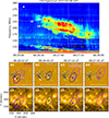 |
Fig. 6. Radio spectrum and temporal evolution of NRH sources of the type II radio burst. (a) CSO/CBSm dynamic spectrum. The white horizontal dashed lines indicate the two NRH imaging frequencies, 173 and 228 MHz. The vertical dashed lines indicate the four selected times shown in the four columns below. The two white dashed curves indicate spectral fitting of the type II burst bands using the Newkirk density model and a shock speed of 800 km s−1. (b1)–(b4) and (c1)–(c4) AIA 171 Å running-difference and original images overplotted with the NRH sources at 173 MHz (magenta) and 228 MHz (dark blue). The contours represent 80% of the maximum brightness temperatures (TBm) and the filled circles denote the centroids of the radio sources from elliptical Gaussian fits. The green curves in panels b2–b4 highlight the wave-like disturbance front. The yellow arrow in panel c1 points to the closed loops. |
The harmonic band splits into two sub-bands, the lower frequency band (LB) and the upper frequency band (UB). The NRH observed the harmonic band of the type II burst at two frequencies, 173 and 228 MHz, as indicated by the two white horizontal dashed lines in Figure 6a. We note that the NRH did not provide imaging at frequencies between 173 and 228 MHz. Here we use the NRH imaging data with an integration time of 1 s.
We now examine the temporal and spatial evolutions of NRH radio sources relative to the jet eruption. NRH sources were overplotted on the AIA 171 Å running-difference and original images at four selected times, as shown in Figures 6b1–b4 and c1–c4, respectively. The maximum brightness temperatures (TBm) of the type II sources are indicated in panels b2–b4. The centroids of the radio sources are determined by applying an elliptical Gaussian fit to the 70% contour levels of the TBm. The uncertainty in the centroid positions should not exceed the pixel size, ∼30″. Due to the jet eruption, the closed loops west of the AR were disturbed. However, the disturbance on the western loops is very weak and cannot be clearly observed, particularly in the original EUV images. From the 1 min cadence EUV running-difference images, we can identify weak signals of the wave-like perturbation front propagating through the closed loops, as highlighted by the green curves in panels b1–b4. Similar jet-induced perturbation fronts can be observed in the running-difference images in 193 Å and 211 Å wavelengths as well.
As shown in Figure 6b1, at 08:26:02 UT, before the onset of the type II burst, the radio sources at both frequencies were initially located near the flare and jet. In panel b2, at the time of the UB backbone, the location of the radio source at 228 MHz shifted to the northwest, coincident with the perturbation front in the EUV running-difference image. Type II bursts are believed to be associated with shock waves. This temporal and spatial coincidence suggests that the observed perturbation induced by the jet eruption is probably a fast-mode shock. In panel b3, the radio source at 228 MHz, representing the herringbones drifting toward high frequencies from the UB, moved toward the southeast. Compared to the UB backbone source, the herringbones are probably located downstream of the shock front, consistent with the physical scenario of herringbones (Holman & Pesses 1983). Later, the radio source in the background at 228 MHz moves back to the position of the jet.
The radio sources at 173 MHz are shown in Figures 6b3 and b4, representing the LB (likely herringbones) and the UB (at a later time), respectively. Both are cospatial with the disturbed loops. The location of the UB at later times moves farther to the northwest, in line with the propagation of the shock over time. The likely LB-associated herringbones, drifting toward lower frequencies from the backbone, are observed to be in the upstream of the shock front, as expected. Because the LB emission exhibits patchy bands and is contaminated by the UB emission, NRH lacks the detection of LB backbone emission for this event. The intermittent characteristics and bumps of the type II burst may be attributed to irregular shock fronts as a result of the inhomogeneity of plasma density in closed loops (Kong et al. 2015; Koval et al. 2023).
To further explore the origin of the shock wave and type II burst, we analyzed the velocities of the jet front and the jet-induced disturbance along the loops. As shown in Figure 7, we selected two cuts in the 171 Å running-difference images to construct the time-distance plots, the red line along the direction of jet eruption and the blue curve along the closed loop. The average speeds were derived by applying a linear fit, as indicated by the dashed lines in panels b and c. The speed of the jet front is ∼246 km s−1 in the plane of the sky. If we assume the inclination angle of the jet relative to the radial direction is 30°, the corrected speed will be ∼500 km s−1. In contrast, the jet-induced perturbation front propagated with a speed of ∼880 km s−1, significantly faster than the jet front.
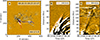 |
Fig. 7. Time–distance plots showing the propagation of the jet front and jet-induced disturbance along the loops. (a) Two cuts along the jet front (red) and the closed loop (blue) in the AIA 171 Å running-difference image. (b) Linear fit (red dashed) to the propagation of the jet front. (c) Propagation speed of the jet-induced wave front (blue dashed). |
We also derived the shock wave speed by performing spectral fitting of the type II burst. Here we apply the Newkik coronal density model Newkirk (1961),
 (1)
(1)
where r is the radial distance from the solar center in units of R⊙. Based on the equation of plasma frequency,
 (2)
(2)
we found that the type II radio spectrum can be nicely fitted with the shock speed of ∼800 km s−1 (see the white dashed curves in Fig. 6), generally consistent with that measured from the time–distance plot of the EUV perturbation front (Fig. 7c). This provides further evidence that the jet-induced perturbation propagating through nearby closed loops acted as the shock driver of the type II radio burst. However, it should be noted that this widely used approach relies on the coronal density model, which has significant uncertainties, particularly in the lower corona.
Coronal structures, such as streamers and loops, are characterized by closed magnetic fields and high plasma density, and thus have a lower Alfvén speed than the ambient corona. The interaction regions between coronal shocks and these structures have been identified as the source regions of both type II radio bursts (e.g., Reiner et al. 2003; Kong et al. 2015; Kouloumvakos et al. 2021; Morosan et al. 2023) and high-energy protons (e.g., Rouillard et al. 2016; Kouloumvakos et al. 2020; Frassati et al. 2022; Liu et al. 2023), due to their higher Alfvénic Mach number and the quasi-perpendicular shock geometry. Using the magnetohydrodynamics model, Morosan et al. (2023) showed that the type II centroids were located in the region with enhanced density inside the streamer, where the minimum Alfvén speed is only ∼100 km s−1. Warmuth & Mann (2005) presented an analytical model of the Alfvén speed in the corona and found regions of minimum Alfvén speed (thus high magnetosonic Mach number) at about 1.2−1.4 R⊙, where the Alfvén speed is generally < 500 km s−1. In our event, the starting frequency of the harmonic emission of the type II burst is about 250 MHz; therefore, we can get the number density Ne ∼ 2 × 108 cm−3 and a height of ∼1.2 R⊙ from Equations (1) and (2). Considering the typical magnetic fields in active region loops, B ∼ 2 − 5 G, we can estimate that the Alfvén speed is about 310−770 km s−1. Compared with the jet-induced perturbation speed ∼880 km s−1, it yields a fast-mode Mach number 1.1−2.8. This suggests that the jet-induced perturbation can steepen into a fast-mode shock wave within low Alfvénic coronal loops.
4. Summary and discussion
In this paper we investigated the origin of a type II radio burst recorded by the CSO/CBSm using multi-wavelength observations. The type II burst was associated with a C-class flare and a small jet, in the absence of a CME. During the impulsive phase of the flare, electrons were accelerated through magnetic reconnection and generated HXR footpoint sources cospatial with the circular ribbons and multiple episodes of type III bursts. A type N burst was observed in the early impulsive phase, while the intense type III burst followed by an interplanetary type III burst occurred around the HXR peak time. NRH imaging shows that the type II radio sources are cospatial with the wave-like perturbation fronts propagating through nearby loops with a speed of ∼880 km s−1, instead of being in front of the jet, as observed in EUV running-difference images. This supports the scenario that a shock wave can form in jet-disturbed surrounding regions with a low Alfvén speed, subsequently accelerating electrons to produce the type II burst. Irregular shock fronts due to the density inhomogeneity of the loops can explain the bumps and patchy structures in the type II emission bands.
Currently, there is an ongoing debate regarding the origin of coronal shock waves that generate metric type II bursts (Vršnak & Cliver 2008). While they are often associated with CME-driven shocks, some events may instead be linked to flare-driven blast waves, jet eruptions, or localized reconnection processes. For the type II event in this study, the solar eruption was a small-scale jet eruption and no clear CME signatures were detected by LASCO/C2 and STEREO/COR1 coronagraphs (angular separation of 9°). We note that this may be attributed to the active region being located close to the solar disk center, as it is affected by projection effects and the field of view of the coronagraphs. Previous studies have also reported that some type II bursts lack CME association (Su et al. 2015; Kumar et al. 2016; Hou et al. 2023; Kumari et al. 2023; Morosan et al. 2023). This suggests that there may exist a specific category of metric type II events at higher starting frequency in which the shock drivers could be different from wide and fast CMEs, therefore changing our traditional paradigm of type II bursts. Future studies combining newly developed solar radioheliographs in the meter and decimeter wavebands are needed to understand the origin and evolution of coronal shocks.
Despite being associated with a small flare, the event still produced electrons with energies up to ∼100 keV, as shown by the Fermi/GBM HXR flux (Fig. 4). This significant phenomenon was also reported in previous studies. Recently, Chen et al. (2025) statistically analyzed 1331 C-class flares recorded by ASO-S/HXI from December 2022 to October 2024. They identified 127 events as high-energy C-class flares, characterized by > 30 keV HXR emission. The event in our study is one of them, in which the HXR flux of ASO-S/HXI exhibits a signal response up to 70 keV. This indicates that despite relatively weak SXR emission, some C-class flares still possess significant capability in nonthermal electron acceleration. Microflares were shown to efficiently accelerate electrons to high energies under specific magnetic field conditions (Ishikawa et al. 2013; Battaglia et al. 2024). For instance, Battaglia et al. (2024) noted that these small flares are typically rooted in sunspots where strong magnetic fields can provide ample energy for magnetic reconnection. However, the specific acceleration mechanism for each individual event requires in-depth analysis.
Our observational results support the fan–spine magnetic topology in the active region. Magnetic reconnection can therefore occur at the coronal null point and near the polarity inversion line where magnetic flux cancellation and shear are observed. During the flare impulsive phase, a fraction of the accelerated electrons propagated outward along the closed filed lines, generating the type N burst and intense type III burst; the other fraction precipitated into the chromosphere, producing the footpoint HXR sources, accompanied by brightening of circular-ribbons in EUV 1600 Å. However, with limited observations of this flare event, it is challenging to determine the exact timing and location of magnetic reconnection and electron acceleration.
Following the onset of the type II radio burst, the Fermi/GBM detected an increase in the 10−25 keV energy range around 08:27 UT (Fig. 4), but no corresponding increase was observed by ASO-S/HXI and no associated HXR source was identified. Recently, Li et al. (2021) explored the possibility that high-energy electrons accelerated by flare reconnection may be further accelerated by CME-shocks. Through interchange reconnection, some flare-accelerated electrons could move to the vicinity of the shock region and be further accelerated, thereby contributing to the generation of type II radio bursts and solar energetic electron events. Based on the current observations, it remains unconfirmed whether the GBM flux enhancement is related to electrons accelerated by the jet-induced shock. As seen from the animation, after the onset of the type II burst, the flare ribbons continued to brighten and expand, indicating that magnetic reconnection was ongoing. Therefore, the increase in GBM flux may be related to the continuous acceleration of electrons by reconnection during the jet eruption process.
Data availability
Movie associated to Fig. 2 is available at https://www.aanda.org
Acknowledgments
X.K. is supported by the National Key R&D Program of China under grant 2022YFF0503002 (2022YFF0503000), the National Natural Science Foundation of China under grants 42074203, and the Qilu Young Scholars Program of Shandong University. Z.L. is supported by the Prominent Postdoctoral Project of Jiangsu Province (2023ZB304). D.Y.D. is supported by NSFC grant 12403065. Z.Z. is supported by NSFC grant 12303061, the Shandong Natural Science Foundation of China (ZR2023QA074), and the China Postdoctoral Science Foundation (2023T160385 and 2022M711931). H.N. is supported by NSFC grant 12203031 and the China Postdoctoral Science Foundation (2022TQ0189). Y.S. is supported by NSFC 12333010. Z.W. is supported by Natural Science Foundation of Shandong Province of China ZR2025MS88. We acknowledge the use of data from the Chinese Meridian Project.
References
- Adams, M., Sterling, A. C., Moore, R. L., & Gary, G. A. 2014, ApJ, 783, 11 [NASA ADS] [CrossRef] [Google Scholar]
- Battaglia, A. F., Krucker, S., Veronig, A. M., et al. 2024, A&A, 691, A172 [NASA ADS] [CrossRef] [EDP Sciences] [Google Scholar]
- Brueckner, G. E., Howard, R. A., Koomen, M. J., et al. 1995, Sol. Phys., 162, 357 [NASA ADS] [CrossRef] [Google Scholar]
- Caroubalos, C., Poquerusse, M., Bougeret, J. L., & Crepel, R. 1987, ApJ, 319, 503 [Google Scholar]
- Chang, S., Wang, B., Lu, G., et al. 2024, ApJS, 272, 21 [Google Scholar]
- Chen, B., Yu, S., Battaglia, M., et al. 2018, ApJ, 866, 62 [Google Scholar]
- Chen, X., Kontar, E. P., Chrysaphi, N., et al. 2020, ApJ, 905, 43 [NASA ADS] [CrossRef] [Google Scholar]
- Chen, C., Su, Y., Chen, W., et al. 2025, ApJ, 987, L4 [Google Scholar]
- Du, G., Chen, Y., Lv, M., et al. 2014, ApJ, 793, L39 [NASA ADS] [CrossRef] [Google Scholar]
- Du, G., Kong, X., Chen, Y., et al. 2015, ApJ, 812, 52 [NASA ADS] [CrossRef] [Google Scholar]
- Duan, Y., Shen, Y., Zhou, X., et al. 2022, ApJ, 926, L39 [NASA ADS] [CrossRef] [Google Scholar]
- Duan, Y., Shen, Y., Tang, Z., Zhou, C., & Tan, S. 2024, ApJ, 968, 110 [Google Scholar]
- Feng, S. W., Chen, Y., Song, H. Q., Wang, B., & Kong, X. L. 2016, ApJ, 827, L9 [Google Scholar]
- Feng, S. W., Xie, H. X., & Misawa, H. 2024, ApJ, 964, 108 [NASA ADS] [CrossRef] [Google Scholar]
- Frassati, F., Laurenza, M., Bemporad, A., et al. 2022, ApJ, 926, 227 [NASA ADS] [CrossRef] [Google Scholar]
- Gan, W.-Q., Zhu, C., Deng, Y.-Y., et al. 2019, RAA, 19, 156 [Google Scholar]
- Ginzburg, V. L., & Zhelezniakov, V. V. 1958, AZh, 35, 694 [NASA ADS] [Google Scholar]
- Glesener, L., Krucker, S., & Lin, R. P. 2012, ApJ, 754, 9 [Google Scholar]
- Holman, G. D., & Pesses, M. E. 1983, ApJ, 267, 837 [NASA ADS] [CrossRef] [Google Scholar]
- Hou, Z., Tian, H., Su, W., et al. 2023, ApJ, 953, 171 [NASA ADS] [CrossRef] [Google Scholar]
- Howard, R. A., Moses, J. D., Vourlidas, A., et al. 2008, Space Sci. Rev., 136, 67 [NASA ADS] [CrossRef] [Google Scholar]
- Ishikawa, S.-N., Krucker, S., Ohno, M., & Lin, R. P. 2013, ApJ, 765, 143 [NASA ADS] [CrossRef] [Google Scholar]
- Kerdraon, A., & Delouis, J. M. 1997, in Coronal Physics from Radio and Space Observations, ed. G. Trottet, 483, 192 [Google Scholar]
- Kong, X., Chen, Y., Guo, F., et al. 2015, ApJ, 798, 81 [Google Scholar]
- Kong, X., Chen, Y., Feng, S., et al. 2016, ApJ, 830, 37 [Google Scholar]
- Kontar, E. P., Chen, X., Chrysaphi, N., et al. 2019, ApJ, 884, 122 [NASA ADS] [CrossRef] [Google Scholar]
- Kontar, E. P., Emslie, A. G., Clarkson, D. L., et al. 2023, ApJ, 956, 112 [NASA ADS] [CrossRef] [Google Scholar]
- Kouloumvakos, A., Rouillard, A. P., Share, G. H., et al. 2020, ApJ, 893, 76 [CrossRef] [Google Scholar]
- Kouloumvakos, A., Rouillard, A., Warmuth, A., et al. 2021, ApJ, 913, 99 [NASA ADS] [CrossRef] [Google Scholar]
- Koval, A., Stanislavsky, A., Karlický, M., et al. 2023, ApJ, 952, 51 [NASA ADS] [CrossRef] [Google Scholar]
- Koval, A., Karlický, M., Brazhenko, A., et al. 2024, A&A, 689, A345 [NASA ADS] [CrossRef] [EDP Sciences] [Google Scholar]
- Kumar, P., Innes, D. E., & Cho, K.-S. 2016, ApJ, 828, 28 [Google Scholar]
- Kumari, A., Morosan, D. E., Kilpua, E. K. J., & Daei, F. 2023, A&A, 675, A102 [NASA ADS] [CrossRef] [EDP Sciences] [Google Scholar]
- Lemen, J. R., Title, A. M., Akin, D. J., et al. 2012, Sol. Phys., 275, 17 [Google Scholar]
- Li, G., Wu, X., Effenberger, F., et al. 2021, Geophys. Res. Lett., 48, e95138 [NASA ADS] [Google Scholar]
- Liu, W., Kong, X., Guo, F., et al. 2023, ApJ, 954, 203 [Google Scholar]
- Lv, M. S., Chen, Y., Li, C. Y., et al. 2017, Sol. Phys., 292, 194 [NASA ADS] [CrossRef] [Google Scholar]
- Magdalenić, J., Marqué, C., Zhukov, A. N., Vršnak, B., & Veronig, A. 2012, ApJ, 746, 152 [Google Scholar]
- Maguire, C. A., Carley, E. P., Zucca, P., Vilmer, N., & Gallagher, P. T. 2021, ApJ, 909, 2 [NASA ADS] [CrossRef] [Google Scholar]
- Mancuso, S., Barghini, D., Bemporad, A., et al. 2023, A&A, 669, A28 [NASA ADS] [CrossRef] [EDP Sciences] [Google Scholar]
- McGlasson, R. A., Panesar, N. K., Sterling, A. C., & Moore, R. L. 2019, ApJ, 882, 16 [NASA ADS] [CrossRef] [Google Scholar]
- Meegan, C., Lichti, G., Bhat, P. N., et al. 2009, ApJ, 702, 791 [Google Scholar]
- Morosan, D. E., Carley, E. P., Hayes, L. A., et al. 2019, Nat. Astron., 3, 452 [Google Scholar]
- Morosan, D. E., Pomoell, J., Kumari, A., Kilpua, E. K. J., & Vainio, R. 2023, A&A, 675, A98 [NASA ADS] [CrossRef] [EDP Sciences] [Google Scholar]
- Nelson, G. J., & Melrose, D. B. 1985, in Solar Radiophysics: Studies of Emission from the Sun at Metre Wavelengths, eds. D. J. McLean, & N. R. Labrum, 333 [Google Scholar]
- Newkirk, G. 1961, ApJ, 133, 983 [NASA ADS] [CrossRef] [Google Scholar]
- Nindos, A., Alissandrakis, C. E., Hillaris, A., & Preka-Papadema, P. 2011, A&A, 531, A31 [NASA ADS] [CrossRef] [EDP Sciences] [Google Scholar]
- Panesar, N. K., Sterling, A. C., Moore, R. L., & Chakrapani, P. 2016, ApJ, 832, L7 [Google Scholar]
- Pesnell, W. D., Thompson, B. J., & Chamberlin, P. C. 2012, Sol. Phys., 275, 3 [Google Scholar]
- Pick, M., & Vilmer, N. 2008, A&ARv, 16, 1 [NASA ADS] [CrossRef] [Google Scholar]
- Reid, H. A. S. 2020, Front. Astron. Space Sci., 7, 56 [NASA ADS] [CrossRef] [Google Scholar]
- Reid, H. A. S., & Kontar, E. P. 2017, A&A, 606, A141 [NASA ADS] [CrossRef] [EDP Sciences] [Google Scholar]
- Reiner, M. J., Vourlidas, A., Cyr, O. C. S., et al. 2003, ApJ, 590, 533 [Google Scholar]
- Rouillard, A. P., Plotnikov, I., Pinto, R. F., et al. 2016, ApJ, 833, 45 [NASA ADS] [CrossRef] [Google Scholar]
- Smerd, S. F., Sheridan, K. V., & Stewart, R. T. 1975, Astrophys. Lett., 16, 23 [NASA ADS] [Google Scholar]
- Sterling, A. C., Moore, R. L., Falconer, D. A., & Adams, M. 2015, Nature, 523, 437 [NASA ADS] [CrossRef] [Google Scholar]
- Su, W., Cheng, X., Ding, M. D., Chen, P. F., & Sun, J. Q. 2015, ApJ, 804, 88 [NASA ADS] [CrossRef] [Google Scholar]
- Su, Y., Liu, W., Li, Y.-P., et al. 2019, RAA, 19, 163 [Google Scholar]
- Su, Y., Zhang, Z., Chen, W., et al. 2024, Sol. Phys., 299, 153 [Google Scholar]
- Vasanth, V. 2024, Sol. Phys., 299, 63 [Google Scholar]
- Vršnak, B., & Cliver, E. W. 2008, Sol. Phys., 253, 215 [Google Scholar]
- Vršnak, B., Aurass, H., Magdalenić, J., & Gopalswamy, N. 2001, A&A, 377, 321 [NASA ADS] [CrossRef] [EDP Sciences] [Google Scholar]
- Warmuth, A., & Mann, G. 2005, A&A, 435, 1123 [NASA ADS] [CrossRef] [EDP Sciences] [Google Scholar]
- Zhang, Q. 2024, Rev. Mod. Plasma Phys., 8, 7 [NASA ADS] [CrossRef] [Google Scholar]
- Zhang, P. J., Wang, C. B., & Ye, L. 2018, A&A, 618, A165 [NASA ADS] [CrossRef] [EDP Sciences] [Google Scholar]
- Zhang, Y., Zhang, Q., Song, D., et al. 2022, ApJS, 260, 19 [Google Scholar]
- Zhong, Z., Guo, Y., Ding, M. D., Fang, C., & Hao, Q. 2019, ApJ, 871, 105 [CrossRef] [Google Scholar]
- Zimovets, I., Vilmer, N., Chian, A. C. L., Sharykin, I., & Struminsky, A. 2012, A&A, 547, A6 [NASA ADS] [CrossRef] [EDP Sciences] [Google Scholar]
All Figures
|
Fig. 1. Overview of the event on 2023 May 8. (a) GOES 1−8 Å soft X-ray light curve (black) of the C3.1-class flare and the ASO−S/HXI count rate from combined total flux detectors (D92+D93+D94) in the 25−50 keV energy channel (orange) between 08:22 and 08:28 UT. (b) Radio dynamic spectrum observed by CSO/CBSm (110−300 MHz), Learmonth (80−110 MHz), and GERMANY-DLR (50−80 MHz), displaying various type III and type III-like (J, N) bursts followed by a type II burst. Both fundamental (F) and harmonic (H) emission lanes can be identified for the type N burst and type II burst. |
| In the text | |
|
Fig. 2. EUV images in the AIA 131 Å, 171 Å, and 304 Å wavelengths (from top to bottom), showing the circular-ribbon flare and jet eruption. The white and black contours in panel c1 respectively represent the positive and negative magnetic fields of the HMI LOS magnetogram scaled at ±120 G. In panel c3 the green and blue curves mark the locations of filaments F1 and F2, respectively, as observed in panel c1. (The associated movie is available online). |
| In the text | |
|
Fig. 3. (a)–(c) GONG Hα images before, during, and after the jet eruption. The white arrows in panel a indicate the two mini-filaments. (d) Evolution of the positive (red) and negative (blue) magnetic flux between 05:20 and 09:10 UT. The gray shaded region indicates the period of the flare. (e) HMI vector magnetic field map at 08:24:00 UT. The red and blue arrows represent the transverse field for positive and negative polarities, respectively. The length of the arrows indicates the magnetic field strength and the direction corresponds to the azimuthal orientation. |
| In the text | |
|
Fig. 4. HXR light curves and imaging of the flare in the duration of radio bursts. (a) ASO-S/HXI count rates of combined total flux detectors (D92+D93+D94) in three energy channels in the range 15−300 keV. (b) Fermi/GBM HXR flux in five channels in the range 4−300 keV. The red dashed lines indicate the peak of the curves at 08:23:52 UT. (c) and (d) Contours of HXR sources from HXI, in energy ranges of 15−25 keV (orange), 20−30 keV (blue), and 30−50 keV (red), overplotted on the AIA 1600 Å and HMI magnetogram images. The contour levels represent 25% and 60% of the maximum. The yellow arrow indicates the positive polarity at the center of the circular ribbon. |
| In the text | |
|
Fig. 5. Radio spectral and imaging observations of the type N burst (harmonic emission). (a) CSO/CBSm radio spectrum, the type N burst is outlined by the black dashed curve. The white dashed lines indicate the three NRH imaging frequencies at 150, 173, and 228 MHz. The red symbols mark the six selected data points shown in panels c and d. (b) Schematic diagram illustrating the generation of a type N burst. The red arrows indicate the propagation directions of the electron beam, while the blue and green curves represent closed and open magnetic field lines, respectively. The ellipses on the closed loop correspond to the radio source locations shown in panels c and d. (c) NRH radio sources superposed on the AIA 193 Å image at three times, as marked by the red dots in panel a. The contours represent 70% of the maximum of each NRH image and are plotted in blue, red, and cyan at three frequencies (150, 173, 228 MHz), respectively. (d) NRH contours corresponding to the data points marked by the red diamond, asterisk, and square in panel a. The white curve represents a schematic of the large-scale closed loop. The yellow arrow points to the position of the jet. |
| In the text | |
|
Fig. 6. Radio spectrum and temporal evolution of NRH sources of the type II radio burst. (a) CSO/CBSm dynamic spectrum. The white horizontal dashed lines indicate the two NRH imaging frequencies, 173 and 228 MHz. The vertical dashed lines indicate the four selected times shown in the four columns below. The two white dashed curves indicate spectral fitting of the type II burst bands using the Newkirk density model and a shock speed of 800 km s−1. (b1)–(b4) and (c1)–(c4) AIA 171 Å running-difference and original images overplotted with the NRH sources at 173 MHz (magenta) and 228 MHz (dark blue). The contours represent 80% of the maximum brightness temperatures (TBm) and the filled circles denote the centroids of the radio sources from elliptical Gaussian fits. The green curves in panels b2–b4 highlight the wave-like disturbance front. The yellow arrow in panel c1 points to the closed loops. |
| In the text | |
|
Fig. 7. Time–distance plots showing the propagation of the jet front and jet-induced disturbance along the loops. (a) Two cuts along the jet front (red) and the closed loop (blue) in the AIA 171 Å running-difference image. (b) Linear fit (red dashed) to the propagation of the jet front. (c) Propagation speed of the jet-induced wave front (blue dashed). |
| In the text | |
Current usage metrics show cumulative count of Article Views (full-text article views including HTML views, PDF and ePub downloads, according to the available data) and Abstracts Views on Vision4Press platform.
Data correspond to usage on the plateform after 2015. The current usage metrics is available 48-96 hours after online publication and is updated daily on week days.
Initial download of the metrics may take a while.