| Issue |
A&A
Volume 706, February 2026
|
|
|---|---|---|
| Article Number | A379 | |
| Number of page(s) | 11 | |
| Section | The Sun and the Heliosphere | |
| DOI | https://doi.org/10.1051/0004-6361/202555337 | |
| Published online | 20 February 2026 | |
STIX observation of chromospheric evaporation
1
Space Research Centre, Polish Academy of Sciences ul. Bartycka 18a 00-716 Warszawa, Poland
2
Astronomical Institute, University of Wrocław ul. Kopernika 11 51-622 Wrocław, Poland
★ Corresponding author: This email address is being protected from spambots. You need JavaScript enabled to view it.
Received:
29
April
2025
Accepted:
11
December
2025
Abstract
Context. Hard X-rays (HXRs) offer the most direct insight into nonthermal electron populations in solar flares, presenting an essential tool for investigating the physical states within flaring structures. The thick-target model suggests that HXR source altitudes in flare footpoints decrease with rising energy due to increased column density. Nonetheless, this relation not depends only on the density, but it is also shaped by the power-law distribution of nonthermal electrons. Furthermore, during the impulsive phase, significant changes in plasma density and ionization levels within footpoints can occur due to heating and chromospheric evaporation, complicating the interpretation of observed HXR footpoint altitudes.
Aims. We aim to investigate the evolution of footpoint source locations for various energy ranges using the most recent measurements collected by the Spectrometer Telescope for Imaging X-rays (STIX).
Methods. Images were reconstructed with the MARLIN algorithm for narrow energy and time bins. For each time and energy interval, images have been reconstructed 101 times, varying detector counts according to their uncertainties. Thus, the source positions were estimated with errors. The absolute reference level (photosphere) has been estimated directly from the analysis of the density distribution derived from the energy-altitude relation.
Results. We found two velocity fields. In the chromosphere, we observed a plateau in the energy-altitude relation that is related to fast mass flow (chromospheric evaporation) up to 250 km s−1. However, with estimated errors in the source positions, at times, we can observe the bump instead of the plateau. If this is indeed a real result, it clearly cannot be explained by the density changes only. In the low corona, we observe a steady flow of plasma, with a velocity of up to 100 km s−1.
Key words: Sun: chromosphere / Sun: corona / Sun: flares / Sun: X-rays / gamma rays
© The Authors 2026
 Open Access article, published by EDP Sciences, under the terms of the Creative Commons Attribution License (https://creativecommons.org/licenses/by/4.0), which permits unrestricted use, distribution, and reproduction in any medium, provided the original work is properly cited.
This article is published in open access under the Subscribe to Open model. This email address is being protected from spambots. You need JavaScript enabled to view it. to support open access publication.
1. Introduction
In a typical flare scenario, the energy stored in magnetic fields is released in the solar corona as the result of to magnetic reconnection. The abrupt change of magnetic field configuration (reconnection) is a cause for the occurrence of dynamic events such as flares, coronal mass ejections (CME), loop oscillations, waves, and so on. The disturbance might cover the entire solar atmosphere (Thompson et al. 1999). Our understanding of solar flares is such that about 40% of the released magnetic energy is transferred to the kinetic energy of electrons (Aschwanden et al. 2016), which deposit it in the chromosphere through interactions with the surrounding plasma via Coulomb collisions. This process is known as the thick-target model (Brown 1971).
The direct result of electron-induced heating of the chromosphere is the expansion of its heated plasma, called chromospheric evaporation. The phenomena was first detected in soft X-ray spectra (SXR; Canfield et al. 1982; Antonucci 1982) as blueshifts produced by the upward-moving plasma. Observed velocities were up to 400 km s−1. The chromospheric evaporation may occur as gentle or explosive (Fisher et al. 1985) depending on the amount of energy deposited by nonthermal electrons. This gives a broad range of expected velocities from a few km s−1 up to several hundred km s−1.
Apart from spectroscopic evidence (e.g., Brosius & Phillips 2004; Milligan et al. 2006a; Doschek et al. 2013; Sellers et al. 2022; Li et al. 2022), numerous observations of vertical movement of flare X-ray footpoints are interpreted as chromospheric evaporation. For example, using YOHKOH/SXT images Tomczak (1997) analyzed the so-called SXR impulsive brightenings (Hudson et al. 1994) in the arcade flare footpoints. He found systematic changes in pixel brightness and estimated the plasma velocity in three footpoints: 460 ± 60, 590 ± 95, and 750 ± 180 km s−1. Statistical analysis of SXR impulsive brightenings (Mrozek & Tomczak 2004) gave the range of velocities 130 − 720 km s−1. The first imaging observation of chromospheric evaporation in the hard X-ray (HXR) was discussed by Silva et al. (1997). The authors compared images from SXT and HXT together with BCS spectra. Moving sources were observed up to energies 14 − 23 keV (HXT’s L channel). HXR sources were observed to be moving with a velocity up to 60 km s−1; however, due to projection effects, the real velocity was higher, up to 200 km s−1, which was observed in the blueshifted component of the Ca XIX line registered by BCS.
The RHESSI observatory (Lin et al. 2002) provided more examples of moving sources observed in HXRs. Liu et al. (2006) analyzed M1.7 SOL20031113T050051 flare. On the X-ray images reconstructed in 12 − 15, 15 − 20, and 20 − 30 keV, they found a change of HXR source brightness along a flare loop. The maximum velocity registered was very high (103 km s−1) but estimated from three data points only. Sui et al. (2006) reports observations of C1.1 SOL20021128T043608 flare visible close to the solar east limb. In the energy range 3 − 6 keV, they observed sources moving upward with the velocity of 340 km s−1. More estimations of chromospheric evaporation velocity were mainly concentrated on the line blueshifts (Milligan et al. 2006a; Li et al. 2017; Sellers et al. 2022) while RHESSI data were used to estimate nonthermal electron beam properties. The obtained values vary from 67–300 km s−1 during downflows to 36 − 60 km s−1 during upflows.
Overall, HXR images with a high energy resolution (i.e., better than a few keV) allow us to test and empirically assess the theoretical correlation between the altitude of HXR footpoint sources and the emitted radiation’s energy (Brown & McClymont 1975). The relation between energy and altitude results from the bremsstrahlung emission process and is influenced by the column density as well as the spectral index of the nonthermal electron beam, as described by Brown et al. (2002). The relation was observed in several investigations including Matsushita et al. (1992), Aschwanden et al. (2002), Matsushita et al. (1992), Aschwanden et al. (2002), Mrozek (2006) and utilized it to derive the density distribution of a flaring loop (Fletcher 1996; Aschwanden et al. 2002). Analyzing HXR source locations provides insights into the physical conditions of a flaring structure. Nonthermal particles serve as a diagnostic tool for investigating plasma across different heights (Kontar et al. 2011). It is important to note that HXR images in the preceding analyses were reconstructed with integration times of at least 40 s. Therefore, the derived density of the vertical structure is averaged over time and it might overlook the plasma dynamics resulting from chromospheric evaporation.
With past HXR telescopes, exploring chromosphere dynamics in high-time and energy resolutions was challenging. For this purpose, we needs a strong flare close to the solar limb and with as simple geometry as possible to avoid doubts in interpretation. Only a few examples have been analyzed (Liu et al. 2006; Mrozek et al. 2022) with time resolutions of 12–24 s for which it was possible to reconstruct RHESSI images with few-keV energy resolution. Assuming plasma density changes dominate the observed changes of source positions, the chromospheric evaporation was analyzed. The velocity and plasma mass (through column density change) were estimated directly from images.
The difficulty of finding flares which are well observed for energy-altitude temporal evolution could potentially be resolved thanks to a new Spectrometer Telescope for Imaging X-rays (STIX; Krucker et al. 2020) installed on board the Solar Orbiter mission. Its angular resolution and dynamic range are not better than those of previous instruments, but its advantage is that it has the capacity to approach the Sun at a distance closer than 0.3 AU. Thus, we expect to observe more details in the energy-altitude. In this study, we concentrated on the solar flare observed by STIX one day after the Solar Orbiter’s perihelion passage. One of the flare’s footpoints was very bright, providing enough count-statistics for the reconstruction of HXR images with time resolution down to 5 seconds, which was never possible for energy-altitude evolution investigation. The close distance to the Sun allowed us to study chromospheric evaporation with a spatial resolution that is better than any previous study of this kind. The observational data are outlined in Sect. 2. Section 3 explains the methodology. Results are detailed in Sect. 4, with conclusions in Sect. 5.
2. Observations and data analysis
STIX is a coded aperture telescope installed on board the Solar Orbiter (Müller et al. 2020) interplanetary mission. Starting from 1 January 2021, STIX continuously records solar HXRs. The observational database currently contains almost 70 000 flares, with a few dozen very strong events recorded close to the orbit’s perihelion. STIX records X-rays in 30 bins covering intervals 4–150 keV using Caliste-Solar Orbiter pixelated detectors (Meuris et al. 2012). The imaging system is based on 30 sub-collimators, which modulate incoming radiation regarding the incident angle. Each sub-collimator consists of a pair of grids that are slightly tilted within a few degrees of each other. The radiation passing through such a system of slits and slats generates a Moiré pattern on the front side of the detectors. This pattern is sampled with a system of 12 pixels (8 large and 4 small) of the detector (Krucker et al. 2020).
The Solar Orbiter’s first scientific orbit started after Earth’s gravitational assist, which took place on 27 November 2021. This maneuver put the Solar Orbiter into orbit with a perihelion distance below 0.33 AU. The first perihelion was reached on 27 March 2022. One day later, a strong solar flare was recorded by STIX. Logarithmically scaled STIX light curves in several energy bands are presented in Fig. 1. Its GOES class was M4.2. The impulsive phase consists of a few HXR bursts, among which the first (above 25 keV) was the strongest and relatively short-lived (∼11:21:06–11:22:06 UT). HXR bursts observed after were slightly weaker and had significantly longer time characteristics. The flare was well-studied by Purkhart et al. (2023). Their studies concern energy release and transport in the flare. Analysis of AIA 1600 Å images was also made to investigate the chromospheric plasma response at the flare footpoints, where the energy from high-energy electrons is deposited. This event was also studied by Morosan et al. (2024) in terms of coronal mass ejection associated with the flare (shock-accelerated electrons). The temporal evolution of the flare-accelerated electrons of this flare has also been studied in detail by Bhattacharjee et al. (2025).
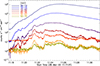 |
Fig. 1. STIX light curves derived from pixel data, background subtracted. Energy bands widths and color coding are presented in the top-left legend. |
The flare was registered by several other telescopes such as SDO/AIA (Lemen et al. 2012) or Solar Orbiter/EUI (Rochus et al. 2020). The longitude separation between the Solar Orbiter and Earth was equal to 81°, giving an excellent overview of flare geometry. Several AIA 171 Å images revealing the morphology of the analyzed flare are presented in Fig. 2 (bottom panels). The first brightenings were observed in a sigmoid-shaped dark structure. From another perspective, EUI 174 Å (Fig. 2, top panels) showed an arc-shaped structure. Next, when the impulsive phase started, the bright loop was visible with precise locations of footpoints. We used these panels to estimate the approximate shape and inclination of a flaring loop visible during the first HXR burst visible from 11:21:06 UT to 11:22:06 UT. Later, the entire morphology became more complicated (arcade shape), which prevented the analysis of single HXR source locations. Moreover, during the first strong HXR burst (electron injection), we may expect that the density distribution in the chromosphere is closest to the nonflaring chromosphere. Further electron injections occur in a more complicated density structure, making the interpretation harder (Mrozek et al. 2022). Therefore, we concentrated only on the first HXR burst, allowing us to trace changes in the flaring atmosphere as they happen.
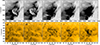 |
Fig. 2. Solar Orbiter/EUI (top row) and SDO/AIA (bottom row) negative images presenting EUV context for the observed event. |
2.1. STIX image reconstructions
STIX image reconstruction is realized in two ways: visibility and count-based (Massa et al. 2023). In this work, we have focused on the MARLIN (Siarkowski et al. 2020) count-based algorithm. We verified the results with other imaging algorithms and found that the relative source positions at individual energies behave consistently. The compatibility of MARLIN with other reconstruction methods is discussed in Litwicka et al. (2025). As STIX is not yet fully calibrated, for image reconstruction, we used sub-collimators Nos. 3–10. The finest grid #3 has an FWHM angular resolution of 14.6″. At the moment of flare observations, the distance of the Solar Orbiter from the Sun was 0.33 AU. It means that 1″ on the solar disc seen from that distance equals 236.6 km. Therefore, even with a resolution of 14.6″, we observe HXR sources with spatial resolution better than 3500 km (4.75″ from a distance of 1 AU). This is better than Yohkoh/HXT FWHM resolution (8″; Kosugi et al. 1991) and is slightly worse than the finest RHESSI resolution, which was expected to be 2.25″ (Hurford et al. 2002). However, in practice, RHESSI images were reconstructed with collimators 3–9 with nominal FWHM resolution 7″ (5000 km spatial resolution). It is worth mentioning that after the full calibration of STIX collimators, including collimators 1 and 2, the FWHM resolution of images will reach 7.1″, which translates into 1680 km spatial resolution for a perihelion distance.
2.2. Stability check of STIX images
We checked the stability of images reconstructed with the MARLIN algorithm as follows. With count-based methods, the input for the reconstruction algorithm is counts recorded in the detector’s stripes A, B, C, and D (Krucker et al. 2020). Having twenty-four detectors (from 3 to 10), we utilized 96 count flux values measured in a given time and energy interval; termed us F[0 : 95]. The uncertainties, containing statistical and compression errors, are also provided after reading fits files, UNC[0 : 95]. These uncertainties have been used to analyze the stability of the image reconstruction; namely, for a given time and energy interval, we perturbed F[0 : 95] values with UNC[0 : 95] in the following manner,
![Mathematical equation: $$ \begin{aligned} FD[0:95] = F[0:95] + COEFF[0:95]*UNC[0:95]. \end{aligned} $$](/articles/aa/full_html/2026/02/aa55337-25/aa55337-25-eq1.gif) (1)
(1)
Here, FD[0 : 95] are fluxes perturbed by uncertainties, and COEFF[0 : 95] are random numbers (uniform distribution) from the interval [ − 1, 1]. Eventually, we got a perturbed set of count fluxes for image reconstruction. The draw of disturbed count fluxes was repeated 101 times and for each set, images were reconstructed. This allowed us to assign errors to parameters (e.g., position) calculated for the image reconstructed in given time and energy intervals. These uncertainties are used further in the paper.
2.3. The loop geometry
After analyzing bright structures in EUV images from 11:21:06 UT to 11:22:06 UT, we estimated the loop parameters in which nonthermal electrons propagate. Figure 3 (panels A and B) shows images recorded by EUI/FSI 174 Å. The images were obtained 5 minutes before and after reconstructed STIX sources, where we can see a system of loops. We outlined the contours of the X-ray sources in 5–7, 16–20, and 36–45 keV energy ranges. We determined the shape of the observed loop from X-ray images (see Fig. 3c), ensuring that all altitudes were accurately corrected for the projection effect to maintain measurement accuracy. We used SDO/AIA and EUI/FSI images to determine the northern footpoint (which is why the loop in Fig. 3c extends beyond the HXR source in the footpoint). Using a simple geometrical method introduced by Loughhead et al. (1983), we estimated the absolute altitude of the loop above the photosphere. For the estimation of the altitude of a loop, we needed to determine its position in the image and identify the reference point (the level of the photosphere), obtained from the footpoint sources. We estimated the height of the loop to be 10 500 km, while the distance between the footpoints was 24 825 km, based on measurements obtained from the image. We confirmed the height of the loop using the method presented in Netzel et al. (2012). Then, assuming that the loop is a perfect ellipse, we corrected the determined altitudes of the HXR sources.
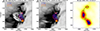 |
Fig. 3. EUI/FSI 174 Å images (negative greyscale) were obtained (a) at 11:10:45 UT and (b) at 11:20:45 UT. Contours of the X-ray sources in 5–7, 16–20, and 36–45 keV energy ranges are outlined on the images (blue, red, and orange solid lines, respectively). The loop was determined manually from STIX images outlined on image 16–20 keV at 11:21:46 UT (black dashed line). Projection effects are more negligible for the southern footpoint (c). |
2.4. Energy-altitude relation and plasma density derivation
The thick-target model is utilized in theoretical contexts to describe a relation involving the altitude of HXR footpoint sources as it refers to the energy of the radiation emitted from such sources (as discussed in detail by Brown & McClymont 1975). The relation arises due to the bremsstrahlung emission process. It is characterized by a dependency on the column density as well as the spectral index of the nonthermal electron beam (Brown et al. 2002).
There are three scenarios for fitting the function to the relation and then obtaining the density. These techniques have been employed by numerous authors (e.g., O’Flannagain et al. 2013; Jeffrey et al. 2014; Mrozek et al. 2022), whose methodology presumes that particles move along the magnetic field lines and that the scattering is neglected.
The first approach is a simple treatment. The column density, N, necessary to stop an electron with energy, E, can be expressed as a function of height based on the observed relation,
 (2)
(2)
where K = 2πe4Λ is constant. The method ignores the spectral dependence and assumes a photon with energy ϵ produced by an electron with energy E. The observed HXR sources are located at different altitudes. Therefore, we can write the formula as follows
 (3)
(3)
We can obtain the density distribution from the relation given by Eq. (3). If we take the derivative d/dz, we get as a result a simple differential relation to obtain the density, n,
 (4)
(4)
Having discrete values of source energy (ϵ) and altitude (z) at hand, we can obtain the density distribution with altitude (Brown et al. 2002):
 (5)
(5)
There is a strong assumption that density is the main parameter defining the shape of the energy-altitude relation. We neglected electron index evolution and other mechanisms (e.g., magnetic mirroring, albedo, etc.). This approach is simple, but very useful for studying the density when the energy-altitude relation cannot be described by a simple analytical function.
The second method involves the fitting of the analytical function to the observations. For example, Aschwanden et al. (2002) fit the observed altitudes of HXR sources as a function of energy with a power law. The observed relation between the photon energy and altitude of the HXR source takes the form of
 (6)
(6)
From this case, we can obtain the changes in the column density with depth given by the formula
 (7)
(7)
where n0 is constant in the form  , and a and z0 are the fitting parameters. We used this approach to analyze the energy-altitude relation obtained from images integrated over long time intervals (up to 60 s) where strong averaging of parameters smears the details and fine structure of the relation. The third and most detailed method assumes electron spectral index dependence. Here, we present the formula written by Brown et al. (2002):
 (8)
(8)
where I0 is scale factor,  ,
,  are the dimensionless parameters, b is free parameter, δ is a spectral slope, and B is the incomplete beta function.
3. Results
3.1. Absolute altitudes of HXR sources
We reconstructed the positions of HXR sources for energies 5–70 keV, for the entire 11:21:06–11:22:06 UT peak (see STIX light curve in Fig. 1). This is the most intense HXR burst detected in higher energies (> 20 keV). We conducted a study of the HXR source that becomes apparent at the footpoint of the solar flare. Figure 4 (top-left panel) shows the 50% isophotes of HXR sources reconstructed for that HXR peak. Energy bands have widths ranging from 3 keV (low energies) up to 20 keV. Centroids of sources within a dotted box marked on the left panel are shown on the right. The energy is denoted by color in a manner that is consistent with the left panel. Linear approximation to the positions and a perpendicular to it, which is the provisional reference level, are indicated. The altitudes above the provisional reference level are presented in the bottom panel of Fig. 4. They have been transformed to kilometers, taking into account the actual Solar Orbiter-to-Sun distance on that day, namely, 0.33 AU. To determine the absolute altitudes of the HXR sources above the photosphere, we used the method described in Mrozek & Kowalczuk (2010). In this way, we were able to fit a power law to the observed energy-altitude relation and derive the density distribution using Eq. (7). The estimated photospheric density altitude (1.16 × 1017 cm−3) was then calculated. Next, we assumed that the altitude of the photospheric level is 0 and applied corrections to the altitudes of HXR sources accordingly. Here, the correction factor is 173 km.
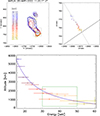 |
Fig. 4. Top-left: Contours of STIX images reconstructed for time interval 11:21:06–11:22:06 UT. Top-right: centroids of sources within a dotted box on the left panel. Linear fits to positions and perpendicular preliminary reference levels are marked accordingly. Energy is color-coded the same way on both panels. Bottom: Energy-altitude relation obtained for points marked in Figure 4. The altitudes have been estimated for corrected reference level, thus they are altitudes above the top of the photosphere. The bump is marked by green square. |
Figure 4 (bottom panel) shows the energy-altitude relation obtained for centroids of the HXR sources in the southern footpoint for the entire examined HXR burst. The fitted power-law function to the observational points is also presented. There is a visible strong deviation from the power law (hereinafter called bump) for higher energies > 30 keV in the energy-altitude relation (Fig. 4, bottom panel). Such a deviation from the power law suggests a more complicated nature of the energy-altitude relation. The relation generally depends on the actual density distribution, so the bump can be caused by the presence of local density disturbances (nonuniform column density distribution) in the loop associated with the chromospheric evaporation. However, the power-law index of the electron spectrum, ionization state, and an unknown ingredient in the magnetic field configuration can also change the altitude of electron thermalization. All these parameters may change during the impulsive phase, so the relation obtained for the entire HXR burst is highly averaged over a more detailed evolution. Since the HXR burst, in the event analyzed here, is strong enough, it can be divided into narrow time intervals. For each of them, the energy-altitude relation can be obtained, as detailed in the next section.
3.2. Energy-altitude relation evolution
We divided the investigated observational time interval of 11:21:06–11:22:06 UT for the HXR burst into subintervals and reconstructed images every 5–10 s, for which we repeated the estimation of the sources’ altitudes (corrected for projection effects) above the photosphere (Figs. 5 and 6). Figure 5 shows the temporal evolution of the relation estimated for all intervals. Using this approach, we can see that for the first four intervals, the relation has a power-law distribution (as we might expect). However, for the next intervals (11:21:41, 11:21:46, 11:21:51 UT), the bump appears and the altitudes get higher over time. The last interval shows the power-law distribution again.
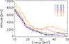 |
Fig. 5. Energy-altitude relations obtained for several time intervals extracted from interval 11:21:06–11:22:06 UT. Time is color-coded. Different evolutions for the chromospheric part end loop leg are visible. Plasma flows in the leg are more gradual, without abrupt changes in velocity. In the chromosphere region, violent reactions to electron beams are visible. |
Figure 6 shows the temporal evolution of the source altitudes for different energies (upper panel) and the evolution of the electron spectrum power-law index (middle panel). We can see that source altitudes evolve in two regimes. Low-energy sources, up to 25 keV, move systematically to higher altitudes. For higher energies, the abrupt rise of altitude is observed after the maximum HXR burst (minimum of the spectral index). For the highest energies (32–56 keV), there is also a significant decrease in the altitude, which is correlated to the spectral index hardening and nonthermal energy flux (Fig. 6, bottom panel).
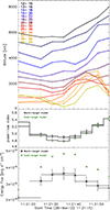 |
Fig. 6. Top: Time evolution of energy-altitude relation for different energies. Middle: Evolution of the nonthermal spectrum power-law index. Bottom: Nonthermal electron energy flux calculated for individual pulses with flare footpoints areas of about 1017 cm2. |
We note that the estimated energy deposited by nonthermal electrons is affected by the choice of target model. The warm-target model provides a more realistic description of electron transport and allows for more accurate estimates of the low-energy cutoff and total injected power (Kontar et al. 2015). In the middle panel of Fig. 6, the power-law index is shown for both the cold-target (green) and warm-target (blue) approaches. The bottom panel presents the corresponding energy fluxes, with the cold-target results marked in green crosses and the warm-target values in black symbols, for direct comparison. The main quantitative differences between the cold- and warm-target models concern the injected electron rate (N0), low-energy cutoff (Ecutoff), and excess emission measure (ΔEM). Since our analysis relies primarily on source altitudes and plasma densities rather than on detailed energetic parameters, the conclusions regarding the evolution of HXR source positions remain unchanged.
According to Eq. (8), two parameters are the main contributors to HXR source altitudes: column density and electron spectral index. Generally, the harder the electron spectral index, the lower the altitude we should observe for a source of a given energy. We noticed the trend for the HXR source altitudes with the spectral index (Fig. 6); it is not clear even for the highest energies. For example, curves representing the sources’ altitudes for energies 32–45, 36–50, and 40–56 keV decrease with spectral index hardening, but this decrease is delayed in time, which is hard to explain with hardening only. Similarly, for rising altitudes, there is a delay in reaction time for different energies, which suggests that density is more important in the evolution of source altitudes. To check this, we employed Eq. (8) to calculate expected altitudes of sources with observed change of electron spectral index (5.0–5.4) and fixed density distribution. The largest change in altitude is found to be ∼200 km for low energy sources (below 25 keV). For higher energies (50 keV), the expected changes due to the observed electron spectral index are much smaller, below 100 km. The observed changes of HXR source altitudes are much larger (> 2500 km for high energy sources). Therefore, we treat the observed range of altitude changes and delay in reaction times as effects directly related to density changes. Assuming that altitudes are related to the column density, we can conclude that from the data in Fig. 5, we can see changes associated with the evolution of plasma density probed by nonthermal electron precipitation.
3.3. Density-altitude relation
The energy-altitude relations (Fig. 5) we used to estimate plasma density distribution along the nonthermal electron path. Because of the complexity of the relations, which are not subject to a power law, we used the simplest approach (Eq. (5)). The density distributions obtained for consecutive subintervals are presented in Fig. 7 with the same color coding as for previous figures. Generally, when the energy-altitude relations are close to a power-law distribution, then the resulting densities are similar to results obtained in Aschwanden et al. (2002). The density changes from roughly 1011 to 1013 cm−3 for altitudes from 5000–6000 km to 600–800 km above the photosphere. The situation is different for the energy-altitude relations with the bump. We can see a sudden increase in the density at 2000–3000 km, which we interpret as the chromospheric plasma moving upwards, namely, the chromospheric evaporation front transiting into the corona. The density evolution fits models of the atmosphere heated by nonthermal electron beams calculated by Nagai & Emslie (1984). A similar pattern of the temporal evolution of the density was obtained in models by Allred et al. (2005), Reep et al. (2015), and Emslie et al. (2024).
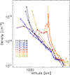 |
Fig. 7. Density evolution for different altitudes obtained for the same time intervals as in Fig. 5. Distributions show clear evaporation front. Time is color-coded. |
Because direct differentiation of noisy observational data leads to large instabilities in the derived density profiles, we introduce an alternative approach for determining the density variation with height. We constructed a grid of theoretical energy–altitude models. Each model consists of two power-law functions smoothly joined at a transition energy and described by the equation,
where A1, A2 are the normalization coefficients, α1, α2 are the power-law indices, h is the HXR emission altitude, and htr is the transition altitude between two regimes. This form provides a simple parametrization consistent with a single rapid density change with height producing a bump in the energy-altitude relation. By varying the normalization coefficients and power-law indices, we generated a grid of models that reflect different plausible scenarios. The resulting curves were additionally smoothed to minimize the effect of the E0(h) discontinuity. From this grid, we selected only those models that best reproduce the observed energy-altitude trends. Using these selected models, we recalculated the density profiles as a function of height. However, it is important to note that the method becomes model-dependent, as it implicitly assumes a specific form of the density distribution with a single discontinuity. Despite this limitation, the results are consistent with the values obtained directly from the observational data (see Fig. 8).
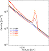 |
Fig. 8. Examples of model-dependent density evolution for different altitudes obtained for the time intervals as in Fig. 5. Time is color-coded. |
3.4. Chromospheric evaporation velocity
Figure 5 and associated Fig. 7 show that the velocity of plasma moving in the flaring loop differs for different parts of a loop. Specifically, for altitudes below 3000 km, we observe the highest velocities up to 250 km s−1. They can be observed for less than 20 s shortly after the maximum of energy deposited by nonthermal electrons. At higher altitudes above the photosphere (> 3000 km), we observe significantly smaller velocities which are below 50 km s−1 before the maximum of deposited nonthermal energy and up to 100 km s−1 after (11:21:40 UT).
In Table A.1, we list the published literature where chromospheric evaporation velocities were reported in the spectral ranges from radio through Hα to X-ray as a reference for our work. The upflows were registered during the impulsive and gradual phases of the solar flares. The table also provides the energy ranges and spectral lines, as well as the instruments used by the authors to determine the upflow velocity. Since the authors did not provide the altitude in the solar atmosphere at which they determined the velocities, we provided (if possible) the logarithm of the temperature (log T) at which the given spectral lines are formed (or the altitudes in a few cases) to clarify which region of the atmosphere chromospheric evaporation was studied in each instance.
4. Discussion
In this work, we analyzed the HXR footpoint source locations related to the source energy (i.e., the energy-altitude relation) and their evolution. In the majority of previous works (Fletcher 1996; Brown et al. 2002; Aschwanden et al. 2002; Mrozek 2006; Kontar et al. 2008, 2010; Battaglia & Kontar 2011), the energy-altitude relation and density structure have been obtained for the entire HXR burst. We repeated this approach for the calibration of source altitudes above the photosphere by fitting the energy-altitude relation to a power-law model (Brown et al. 2002; Aschwanden et al. 2002).
We observed a bump in the energy-altitude relation obtained for the entire HXR burst, which exhibited a more complicated nature of the relation. Having STIX much closer to the Sun increases count statistics, thus, we can now see details of the temporal evolution of the relation during a single HXR burst. We reconstructed HXR images in short time intervals (5–10 s) and narrow energy intervals (3–10 keV). Their altitudes above the photosphere showed new features that we had not observed in the past in the HXRs. It can be noted (Fig. 5) that for ∼11:21:16, 11:21:26, and 11:21:31 UT, the relation has a power-law distribution, as we might expect. However, for the next three time intervals, a bump appeared (the altitudes getting higher with time). The last interval shows a power-law distribution again. The origin of the bump may be related to several parameters, which are from nonthermal electron beam properties and the state of the target atmosphere. Moreover, the albedo may affect the reconstructed source parameters (e.g., position, size; Battaglia et al. 2011); namely, the photon backscattering from the photosphere (Kontar & Jeffrey 2010).
The effect of albedo should always be considered when the sizes or positions of X-ray sources are analyzed. Among other parameters, the displacement of the HXR source position is energy-dependent and related to the radial distance from the solar disc center. The flare analyzed here was observed at μ ∼ 0.17, while the bump is a feature occurring in the energy range 30–50 keV. According to Kontar & Jeffrey (2010), the displacement observed in the range 20–50 keV at μ ∼ 0.1–0.2 is 0.2–0.7 arc sec, depending on the degree of anisotropy of the source emission. Considering that a source’s position shifts due to albedo is always towards the solar disc centre, the bump we observe is an effect in the opposite direction, namely, it is facing away from the disc centre.
The main factors influencing the height of HXR sources and potentially responsible for the observed bump primarily include the column density and the nonthermal electron spectrum’s power-law index (Brown et al. 2002). As we discuss in Sect. 3.2, the power-law index for the analyzed event is seen to change from 4.8 to 5.6. Assuming a steady density structure, the power-law index of the electron beam spectrum could generate changes in the altitude at a level of 200 km for 15 keV and 400 km for 30 keV sources. For the region of the bump occurrence, it is less than 100 km, which is far below the observed range of altitude changes (around 2500 km). Therefore, in the remainder of the discussion, we focus on observed changes that are density-related only.
The observed energy-altitude relation’s evolution shows the density changes in a large part of the flare half-loop (i.e., the loop connecting the top with the southern footpoint). Utilizing nonthermal electrons as a tool, we can probe the density with very high precision. From a simple comparison of energy-altitude relations obtained for different moments in time, we see that two regions with different velocities exist in the flaring loop. There is almost a steady flow of plasma in the coronal part of the loop (> 3000 km, loop sources) and a more abrupt, high-velocity region located below (< 3000 km, footpoint sources). Loop sources are mainly observed in the energies 10–20 keV and we expect a strong influence of the thermal emission in this range. Indeed, the spectral analysis revealed that for that event, the clear nonthermal emission is observed above 18 keV. Thus, we expect that the low-energy part of the energy-altitude relation gives us mainly information about hot plasma flowing up in the flaring loop. The estimated velocities are in the range of 50 − 100 km s−1 depending on the phase of the HXR burst (i.e., they are lower before the burst’s maximum and reach 100 km s−1 after the maximum). These velocities are partly consistent with previous results presented in Table A.1, where we collected results from several papers related to the observations of the chromospheric evaporation. Spectral lines forming in the hot plasma often show similar values (below 100 km s−1), but there are also results (e.g., Antonucci 1982; Canfield et al. 1982; Milligan & Dennis 2009) presenting velocities well above 200 km s−1. However, we have to remember that formation temperature cannot be simply translated to altitude. For example, there are observations based on soft X-ray images (Tomczak 1997; Silva et al. 1997; Mrozek & Tomczak 2004) which revealed 60 − 750 km s−1 velocities in the footpoints observed SXR region. Such “hot footpoints” are interesting from the point of view of the nonthermal energy beam deposition, as they are hot targets for electrons (Brown & Mallik 2009; Emslie 2003).
From a theoretical point of view, the dichotomy of chromospheric evaporation (i.e., explosive vs. gentle) was first discussed by Fisher et al. (1985). The limit value of the beam’s energy, which results in the explosive evaporation coined by Fisher et al. (1985), is equal to 7 × 10⁹ erg cm−2 s−1. For the purposes of a simple comparison, we estimated the beam energy. Assuming a single power-law electron distribution, we obtained the non-thermal electron energy flux for individual pulses. From individual images, we estimated the ranges of flare footpoint areas which have values between 1.93 × 1017 cm2 and 2.98 × 1017 cm2. The obtained area range allowed us to determine possible values of the beam energy (in erg cm−2 s−1) for each moment presented in Fig. 6 (bottom panel). For each point, we determined both the maximum and minimum values of the beam energy according to a range of estimated areas. It follows that the determined values of the energy flux are greater than the critical value for each of the intervals analyzed in this work, namely, explosive evaporation occurs.
Despite the fact that explosive evaporation threshold was reached, we also observed simultaneously lower velocities in the coronal part of the flaring loop. Such a behavior can be explained by models that include the effects of turbulence on energy release and transport in solar flares, as in the study by Emslie et al. (2024). Their key findings indicate that turbulence plays a significant role in changing the solar atmosphere’s response to flare energy input, leading to rapid heating of the corona to high temperatures and sustaining elevated temperatures post-energy input, causing overpressure in the corona and impeding the upward motions of chromospheric plasma.
Based on the temporal evolution of the energy-altitude relation, we obtained a density evolution for each time interval (Fig. 7). We can see that the evolution corresponds to the changes in the relation. A large density gradient occurring at ∼11:21:46 UT and ∼11:21:51 UT indicates significant disturbances in the loop. Employing the model by Nagai & Emslie (1984) with the density evolution 10–15 seconds after the electron beam was released, we obtained results of the distributions on a similar time scale for the STIX observational cadence of similar ranges (10–15 s). We observed that there is a strong front at lower altitudes and gentle flow at higher altitudes, but the front remains in the model.
The details of the plasma flows in the flaring loop revealed by the STIX data are very important from the nonthermal energy deposition depth point of view, giving additional constraints to flaring atmosphere models. The energy deposition site (limited plasma volume) evolves in time in terms of height in the loop and in terms of width due to chromospheric evaporation and material moving towards the corona. The temporal evolution of the position of such a layer in the loop and its expansion and contraction were investigated, utilizing HXR observations from RHESSI, presented in the work of Radziszewski et al. (2020). The layer expanded from 500 to 1625 km above the temperature minimum. If the layer in which the energy is deposited begins to expand and the density in it increases (as can be seen in our analysis). Then, it is plausible that the subsequent nonthermal electron beams that move towards the chromosphere do not have enough energy (i.e., there is a small amount of energetic electrons that penetrate deep into the chromosphere and they penetrate the chromospheric front, but most electrons in the beam have low energies and do not pass further) to penetrate the previously created high plasma density.
The precise determination of HXR source altitudes changes dramatically when estimated for the entire HXR burst or finer time bins. Figures 4 and 5 show that whole-burst reconstructions and source positions follow a power law within error bars. However, our analysis, which reconstructs sources for the burst into small intervals, reveals significantly different positions for some of the analyzed time intervals. We find that positions in the range 30–50 keV can differ by 2500 km in the time scale of 10 s. This is extremely important when comparing this with observations in other wavelengths and the interpretation of absolute positions of HXR sources above the photosphere (e.g., Battaglia & Kontar 2011; Martínez Oliveros et al. 2012). Potentially, detailed HXR analysis of plasma dynamics and energy deposition levels might help to solve many complex spectroscopic observations (see discussion in Doschek et al. 2013), where the observed hot plasma emissions are strongly related to the site of maximum energy deposition. In our work, we show an example to demonstrate that HXR observations should be analyzed with as narrow time intervals and energy bands as possible. For example, the importance of time interval selection was recently shown by Battaglia & Krucker (2025), thereby resolving a 20-year-long mystery regarding the positions of HXR and gamma footpoint sources.
5. Summary
This study examines the energy-altitude relation of HXR sources at footpoints and their evolution, emphasizing the complexity of this relation. Previous research took into account the entire HXR burst using a power-law model. By studying HXR sources observed by STIX when it was closer to the Sun with better count statistics, research has revealed temporal evolution details within a single HXR burst. By reconstructing HXR images in narrow time and energy intervals, new altitude characteristics have appeared, including a noticeable increase in the energy-altitude relation at specified intervals (i.e., the appearance of the bump ∼30 s after the HXR emission start), velocity dichotomy during chromospheric evaporation, and density distribution.
The dynamics of chromospheric evaporation observed during the flare provide critical insights into how energy deposited by nonthermal electrons can lead to significant changes in plasma behavior. The observed bump in the energy-altitude relation challenges existing models that rely on simpler power-law distributions, indicating that more complex interactions and conditions within the solar atmosphere must be considered. The distinct velocity fields highlight the layered structure of the solar atmosphere and underscore the importance of time-resolution measurements in capturing the rapid changes occurring during flare events. The ability to derive density distributions enhances our understanding of the physical conditions within flaring loops.
Electrons serve as a valuable tool for probing the levels of energy deposition in solar flares and the subsequent response of the solar atmosphere, particularly in terms of chromospheric evaporation. Beams of high-energy particles moving in the solar atmosphere make it possible to study the dynamics and physical properties of flare plasma (e.g., plasma density distribution in flare loops). The study indicated that by analyzing the energy-altitude relation of HXR footpoint sources, we could gain insights into the dynamics of plasma flows and density changes in the chromosphere and corona. This approach allows for a detailed understanding of how nonthermal electrons influence the heating and movement of plasma in the solar atmosphere.
In general, our results are consistent with previous works, particularly with studies based on images in the HXR energy range (e.g., Silva et al. 1997; Mrozek & Tomczak 2004). In addition, we can clearly see that the chromospheric evaporation rate decreases with altitude. The emergence of two velocity fields is an open question that ought to be further investigated via data-driven modeling. From a data analysis point of view, we are in the process of performing a statistical analysis of the events leading up to the appearance of the bump during HXR bursts.
Acknowledgments
Solar Orbiter is a space mission of international collaboration between ESA and NASA, operated by ESA. The STIX instrument is an international collaboration between Switzerland, Poland, France, the Czech Republic, Germany, Austria, Ireland, and Italy. This work was supported by the Polish National Science Center grant number 2020/39/B/ST9/01591. TM is supported by the Polish National Science Center grant number 2023/49/B/ST9/02409. We thank the anonymous referee for helpful comments and suggestions that improved the manuscript.
References
- Allred, J. C., Hawley, S. L., Abbett, W. P., & Carlsson, M. 2005, ApJ, 630, 573 [NASA ADS] [CrossRef] [Google Scholar]
- Antonucci, E. 1982, Mem. Soc. Astron. It., 53, 495 [NASA ADS] [Google Scholar]
- Aschwanden, M. J., Brown, J. C., & Kontar, E. P. 2002, Sol. Phys., 210, 383 [Google Scholar]
- Aschwanden, M. J., Holman, G., O’Flannagain, A., et al. 2016, ApJ, 832, 27 [Google Scholar]
- Battaglia, M., & Kontar, E. P. 2011, ApJ, 735, 42 [Google Scholar]
- Battaglia, A. F., & Krucker, S. 2025, A&A, 694, A58 [NASA ADS] [CrossRef] [EDP Sciences] [Google Scholar]
- Battaglia, M., Kontar, E. P., & Hannah, I. G. 2011, A&A, 526, A3 [NASA ADS] [CrossRef] [EDP Sciences] [Google Scholar]
- Berlicki, A., Heinzel, P., Schmieder, B., Mein, P., & Mein, N. 2005, A&A, 430, 679 [NASA ADS] [CrossRef] [EDP Sciences] [Google Scholar]
- Bhattacharjee, D., Kontar, E. P., & Luo, Y. 2025, ApJ, 987, 211 [Google Scholar]
- Brosius, J. W., & Phillips, K. J. H. 2004, ApJ, 613, 580 [Google Scholar]
- Brown, J. C. 1971, Sol. Phys., 18, 489 [Google Scholar]
- Brown, J. C., & Mallik, P. C. V. 2009, ApJ, 697, L6 [Google Scholar]
- Brown, J. C., & McClymont, A. N. 1975, Sol. Phys., 41, 135 [NASA ADS] [CrossRef] [Google Scholar]
- Brown, J. C., Aschwanden, M. J., & Kontar, E. P. 2002, Sol. Phys., 210, 373 [NASA ADS] [CrossRef] [Google Scholar]
- Canfield, R. C., Gunkler, T. A., Hudson, H. S., et al. 1982, Adv. Space Res., 2, 145 [NASA ADS] [CrossRef] [Google Scholar]
- Czaykowska, A., De Pontieu, B., Alexander, D., & Rank, G. 1999, ApJ, 521, L75 [Google Scholar]
- del Zanna, G., Schmieder, B., Mason, H., Berlicki, A., & Bradshaw, S. 2006, Sol. Phys., 239, 173 [Google Scholar]
- Doschek, G. A., Warren, H. P., & Young, P. R. 2013, ApJ, 767, 55 [NASA ADS] [CrossRef] [Google Scholar]
- Emslie, A. G. 2003, ApJ, 595, L119 [NASA ADS] [CrossRef] [Google Scholar]
- Emslie, A. G., Allred, J. C., & Alaoui, M. 2024, ApJ, 977, 246 [Google Scholar]
- Fisher, G. H., Canfield, R. C., & McClymont, A. N. 1985, ApJ, 289, 414 [NASA ADS] [CrossRef] [Google Scholar]
- Fletcher, L. 1996, A&A, 310, 661 [NASA ADS] [Google Scholar]
- Hudson, H. S., Strong, K. T., Dennis, B. R., et al. 1994, ApJ, 422, L25 [Google Scholar]
- Hurford, G. J., Schmahl, E. J., Schwartz, R. A., et al. 2002, Sol. Phys., 210, 61 [Google Scholar]
- Jeffrey, N. L. S., Kontar, E. P., Bian, N. H., & Emslie, A. G. 2014, ApJ, 787, 86 [NASA ADS] [CrossRef] [Google Scholar]
- Kontar, E. P., & Jeffrey, N. L. S. 2010, A&A, 513, L2 [NASA ADS] [CrossRef] [EDP Sciences] [Google Scholar]
- Kontar, E. P., Hannah, I. G., & MacKinnon, A. L. 2008, A&A, 489, L57 [NASA ADS] [CrossRef] [EDP Sciences] [Google Scholar]
- Kontar, E. P., Hannah, I. G., Jeffrey, N. L. S., & Battaglia, M. 2010, ApJ, 717, 250 [NASA ADS] [CrossRef] [Google Scholar]
- Kontar, E. P., Brown, J. C., Emslie, A. G., et al. 2011, Space Sci. Rev., 159, 301 [NASA ADS] [CrossRef] [Google Scholar]
- Kontar, E. P., Jeffrey, N. L. S., Emslie, A. G., & Bian, N. H. 2015, ApJ, 809, 35 [NASA ADS] [CrossRef] [Google Scholar]
- Kosugi, T., Makishima, K., Murakami, T., et al. 1991, Sol. Phys., 136, 17 [NASA ADS] [CrossRef] [Google Scholar]
- Krucker, S., Hurford, G. J., Grimm, O., et al. 2020, A&A, 642, A15 [NASA ADS] [CrossRef] [EDP Sciences] [Google Scholar]
- Lemen, J. R., Title, A. M., Akin, D. J., et al. 2012, Sol. Phys., 275, 17 [Google Scholar]
- Li, D., Ning, Z. J., Huang, Y., & Zhang, Q. M. 2017, ApJ, 841, L9 [NASA ADS] [CrossRef] [Google Scholar]
- Li, D., Hong, Z., & Ning, Z. 2022, ApJ, 926, 23 [NASA ADS] [CrossRef] [Google Scholar]
- Li, D., Li, C., Qiu, Y., et al. 2023, ApJ, 954, 7 [Google Scholar]
- Lin, R. P., Dennis, B. R., Hurford, G. J., et al. 2002, Sol. Phys., 210, 3 [Google Scholar]
- Litwicka, M., Mrozek, T., Awasthi, A. K., et al. 2025, ApJ, 985, 29 [Google Scholar]
- Liu, W., Liu, S., Jiang, Y. W., & Petrosian, V. 2006, ApJ, 649, 1124 [NASA ADS] [CrossRef] [Google Scholar]
- Loughhead, R. E., Wang, J. L., & Blows, G. 1983, ApJ, 274, 883 [Google Scholar]
- Martínez Oliveros, J.-C., Hudson, H. S., Hurford, G. J., et al. 2012, ApJ, 753, L26 [CrossRef] [Google Scholar]
- Massa, P., Hurford, G. J., Volpara, A., et al. 2023, Sol. Phys., 298, 114 [NASA ADS] [CrossRef] [Google Scholar]
- Matsushita, K., Masuda, S., Kosugi, T., Inda, M., & Yaji, K. 1992, PASJ, 44, L89 [NASA ADS] [Google Scholar]
- Meuris, A., Hurford, G., Bednarzik, M., et al. 2012, Nucl. Instrum. Methods Phys. Res., 695, 288 [Google Scholar]
- Milligan, R. O., & Dennis, B. R. 2009, ApJ, 699, 968 [NASA ADS] [CrossRef] [Google Scholar]
- Milligan, R. O., Gallagher, P. T., Mathioudakis, M., et al. 2006a, ApJ, 638, L117 [NASA ADS] [CrossRef] [Google Scholar]
- Milligan, R. O., Gallagher, P. T., Mathioudakis, M., & Keenan, F. P. 2006b, ApJ, 642, L169 [NASA ADS] [CrossRef] [Google Scholar]
- Morosan, D. E., Pomoell, J., Palmroos, C., et al. 2024, A&A, 683, A31 [NASA ADS] [CrossRef] [EDP Sciences] [Google Scholar]
- Mrozek, T. 2006, Adv. Space Res., 38, 962 [NASA ADS] [CrossRef] [Google Scholar]
- Mrozek, T., & Kowalczuk, J. 2010, Cent. Eur. Astrophys. Bull., 34, 57 [Google Scholar]
- Mrozek, T., & Tomczak, M. 2004, A&A, 415, 377 [NASA ADS] [CrossRef] [EDP Sciences] [Google Scholar]
- Mrozek, T., Falewicz, R., Kołomański, S., & Litwicka, M. 2022, A&A, 659, A60 [NASA ADS] [CrossRef] [EDP Sciences] [Google Scholar]
- Müller, D., St. Cyr, O. C., Zouganelis, I., et al. 2020, A&A, 642, A1 [Google Scholar]
- Nagai, F., & Emslie, A. G. 1984, ApJ, 279, 896 [Google Scholar]
- Netzel, A., Mrozek, T., Kołomański, S., & Gburek, S. 2012, A&A, 548, A89 [NASA ADS] [CrossRef] [EDP Sciences] [Google Scholar]
- Ning, Z. J. 2011, ASI Conf. Ser., 2, 279 [Google Scholar]
- Ning, Z., Cao, W., Huang, J., et al. 2009, ApJ, 699, 15 [Google Scholar]
- O’Flannagain, A. M., Gallagher, P. T., Brown, J. C., Milligan, R. O., & Holman, G. D. 2013, A&A, 555, A21 [NASA ADS] [CrossRef] [EDP Sciences] [Google Scholar]
- Purkhart, S., Veronig, A. M., Dickson, E. C. M., et al. 2023, A&A, 679, A99 [NASA ADS] [CrossRef] [EDP Sciences] [Google Scholar]
- Radziszewski, K., Falewicz, R., & Rudawy, P. 2020, ApJ, 903, 28 [Google Scholar]
- Reep, J. W., Bradshaw, S. J., & Alexander, D. 2015, ApJ, 808, 177 [NASA ADS] [CrossRef] [Google Scholar]
- Rochus, P., Auchère, F., Berghmans, D., et al. 2020, A&A, 642, A8 [NASA ADS] [CrossRef] [EDP Sciences] [Google Scholar]
- Sadykov, V. M., Vargas Dominguez, S., Kosovichev, A. G., et al. 2015, ApJ, 805, 167 [Google Scholar]
- Schmieder, B., Malherbe, J. M., Simnett, G. M., Forbes, T. G., & Tandberg-Hanssen, E. 1990, ApJ, 356, 720 [NASA ADS] [CrossRef] [Google Scholar]
- Sellers, S. G., Milligan, R. O., & McAteer, R. T. J. 2022, ApJ, 936, 85 [Google Scholar]
- Siarkowski, M., Mrozek, T., Sylwester, J., Litwicka, M., & Dąbek, M. 2020, Open Astron., 29, 220 [NASA ADS] [CrossRef] [Google Scholar]
- Silva, A. V. R., Wang, H., Gary, D. E., Nitta, N., & Zirin, H. 1997, ApJ, 481, 978 [NASA ADS] [CrossRef] [Google Scholar]
- Sui, L., Holman, G. D., & Dennis, B. R. 2006, ApJ, 645, L157 [NASA ADS] [CrossRef] [Google Scholar]
- Thompson, B. J., Gurman, J. B., Neupert, W. M., et al. 1999, ApJ, 517, L151 [Google Scholar]
- Tomczak, M. 1997, A&A, 317, 223 [NASA ADS] [Google Scholar]
Appendix A: Chromospheric evaporation velocities
Chromospheric evaporation velocities from selected publications.
All Tables
All Figures
|
Fig. 1. STIX light curves derived from pixel data, background subtracted. Energy bands widths and color coding are presented in the top-left legend. |
| In the text | |
|
Fig. 2. Solar Orbiter/EUI (top row) and SDO/AIA (bottom row) negative images presenting EUV context for the observed event. |
| In the text | |
|
Fig. 3. EUI/FSI 174 Å images (negative greyscale) were obtained (a) at 11:10:45 UT and (b) at 11:20:45 UT. Contours of the X-ray sources in 5–7, 16–20, and 36–45 keV energy ranges are outlined on the images (blue, red, and orange solid lines, respectively). The loop was determined manually from STIX images outlined on image 16–20 keV at 11:21:46 UT (black dashed line). Projection effects are more negligible for the southern footpoint (c). |
| In the text | |
|
Fig. 4. Top-left: Contours of STIX images reconstructed for time interval 11:21:06–11:22:06 UT. Top-right: centroids of sources within a dotted box on the left panel. Linear fits to positions and perpendicular preliminary reference levels are marked accordingly. Energy is color-coded the same way on both panels. Bottom: Energy-altitude relation obtained for points marked in Figure 4. The altitudes have been estimated for corrected reference level, thus they are altitudes above the top of the photosphere. The bump is marked by green square. |
| In the text | |
|
Fig. 5. Energy-altitude relations obtained for several time intervals extracted from interval 11:21:06–11:22:06 UT. Time is color-coded. Different evolutions for the chromospheric part end loop leg are visible. Plasma flows in the leg are more gradual, without abrupt changes in velocity. In the chromosphere region, violent reactions to electron beams are visible. |
| In the text | |
|
Fig. 6. Top: Time evolution of energy-altitude relation for different energies. Middle: Evolution of the nonthermal spectrum power-law index. Bottom: Nonthermal electron energy flux calculated for individual pulses with flare footpoints areas of about 1017 cm2. |
| In the text | |
|
Fig. 7. Density evolution for different altitudes obtained for the same time intervals as in Fig. 5. Distributions show clear evaporation front. Time is color-coded. |
| In the text | |
|
Fig. 8. Examples of model-dependent density evolution for different altitudes obtained for the time intervals as in Fig. 5. Time is color-coded. |
| In the text | |
Current usage metrics show cumulative count of Article Views (full-text article views including HTML views, PDF and ePub downloads, according to the available data) and Abstracts Views on Vision4Press platform.
Data correspond to usage on the plateform after 2015. The current usage metrics is available 48-96 hours after online publication and is updated daily on week days.
Initial download of the metrics may take a while.