| Issue |
A&A
Volume 706, February 2026
|
|
|---|---|---|
| Article Number | A299 | |
| Number of page(s) | 11 | |
| Section | Astrophysical processes | |
| DOI | https://doi.org/10.1051/0004-6361/202555394 | |
| Published online | 18 February 2026 | |
The role of distant pulsars in the detectability of continuous gravitational waves
1
Max-Planck-Institut für Radioastronomie Auf dem Hügel 69 D-53121 Bonn, Germany
2
Sternberg Astronomical Institute, Moscow State University, Universitetsky Pr. 13 Moscow 119234, Russia
3
Jodrell Bank Centre for Astrophysics, University of Manchester, Department of Physics and Astronomy, Alan-Turing Building Oxford Street Manchester M13 9PL, UK
★ Corresponding author: This email address is being protected from spambots. You need JavaScript enabled to view it.
Received:
5
May
2025
Accepted:
4
January
2026
Abstract
Context. One of the imminent science goals of pulsar timing arrays (PTAs) is the detection of a continuous gravitational wave (CGW) emitted by an individual supermassive black hole binary (SMBHB). SMBHBs that cause CGWs with GW frequencies fGW > 10 nHz (high-frequency end of the nano-Hertz GW spectrum) have undergone significant orbital evolution and hence a change in fGW over time. In PTA datasets with a sufficiently long observational time span, this means that the contributions of the Earth and the pulsar terms to the CGW signal signature can eventually become resolvable. Since the pulsar term is accumulated incoherently and thus often treated as an additional source of noise, this separation can prove to be beneficial for the detection of the CGW signal in the PTA dataset.
Aims. We investigate to which extent resolvable Earth and pulsar terms affect currently used techniques for CGW searches with PTA datasets, which treat the pulsar term as an additional source noise. We focus on the dependence of the pulsar term frequencies on the pulsar distance. We aim to answer the question of whether adding more distant pulsars to a PTA dataset can mitigate biases and improve the detection of CGWs.
Methods. We used simulated PTA datasets based on the EPTA DR2 and IPTA DR2 pulsars in order to study the performance of the Earth-term-only Bayesian parameter estimation of the circular SMBHB model parameters and the frequentist narrow-band optimal statistic in the light of resolved pulsar terms due to larger pulsar distances.
Results. We show that under ideal conditions, more distant pulsars can facilitate the CGW search with PTA datasets. The Bayesian parameter estimation is yielding better parameter constraints, and the frequentist search becomes more stable. Based on realistic dataset simulations, however, we found that other configuration parameters of a PTA, such as the anisotropic distribution of pulsars and the effective number of pulsars in a PTA, can play a crucial role in the importance of this effect.
Key words: gravitational waves / methods: numerical / pulsars: general
© The Authors 2026
 Open Access article, published by EDP Sciences, under the terms of the Creative Commons Attribution License (https://creativecommons.org/licenses/by/4.0), which permits unrestricted use, distribution, and reproduction in any medium, provided the original work is properly cited.
This article is published in open access under the Subscribe to Open model.
Open access funding provided by Max Planck Society.
1. Introduction
The direct detection of a gravitational wave (GW) originating from the interaction of a black-hole binary allows us to draw conclusions about the masses of the components, the orientation of the binary, and the distance and eccentricity by analysing the measured wave form (Maggiore 2000). Results of GW searches in the past decade were dominated by the detection of GWs in the high-frequency regime (1 Hz to 1000 Hz) caused by merging stellar mass black-hole binaries with ground-based interferometers (Bailes et al. 2021). In addition to the high-frequency GW regime, significant efforts were made over the past decades to also detect GWs at lower frequencies (fGW ∼ nHz). These low-frequency GWs can originate from supermassive black hole (SMBH) binaries (Rajagopal & Romani 1995). These SMBHs are expected to be found in the centres of galaxies (Begelman et al. 1980; Kormendy & Richstone 1995; Milosavljević & Merritt 2001), and their GW fingerprint can thus serve as a tracer of galaxy interaction and formation history (Burke-Spolaor 2015). To detect these low-frequency GWs, a galaxy-sized GW detector is needed.
The so-called Pulsar Timing Arrays (PTAs) provide this type of detector by exploiting the highly predictable rotational behaviour of millisecond pulsars (Estabrook & Wahlquist 1978; Sazhin 1978; Detweiler 1979; Foster & Backer 1990). Pulsar timing describes the method of exploiting the extraordinary rotational stability of millisecond pulsars by precisely recording their pulse arrival times (ToAs) at the radio telescope using maser clocks tied to international time standards, and comparing the measured time series to the one predicted by the timing model (e.g. Lorimer & Kramer 2005). The deviations between measurement and model, the so-called timing residuals, are then used to determine the model parameters, such as the astrometric or orbital parameters, to unmatched precision. With typical observation time spans of some dozen years, PTA datasets allow for the analysis of periodic signals ranging in frequencies from fmin = 1/Tobs ∼ nHz to the Nyquist frequency 1/(2Δtobs) determined by the observational cadence of the PTA. A typical cadence of monthly observations sets the upper signal frequency limit of a PTA to ∼100 nHz.
By combining the ToA measurements and timing models of several pulsars, it is possible to search for the pulsar residuals induced by GWs in the nano-Hertz regime. The degree of correlation of the GW-induced delays, the overlap reduction function, follows, the Hellings-Downs (HD) curve (Hellings & Downs 1983) as a function of the angular pulsar separation, under the assumption of GR. This correlation function is the fingerprint of GWs in the dataset. The GW analysis of a PTA is built upon the Fourier decomposition of the dataset, where the Fourier frequencies are multiples of fmin, also referred to as frequency bins.
The two main GW signals that are searched for using PTAs are (i) the stochastic gravitational wave background (GWB), which manifests as a stochastic common red-noise signal in the pulsar timing residuals (see e.g. Allen & Romano 1999; Phinney 2001; Jaffe & Backer 2003), and (ii) continuous gravitational waves (CGWs) originating from individual SMBHB inspirals, which produce a deterministic correlated wave-like pattern in the residuals (Foster & Backer 1990; Sesana & Vecchio 2010; Ravi et al. 2012). Both signals are expected to be HD correlated (Romano & Allen 2024).
Based on realistic simulations of cosmological population of SMBHs, it was found that the first source that is expected to be detected in the PTA band is the GWB (Rosado et al. 2015). In June 2023, various PTA collaborations around the world published compelling evidence for the presence of an HD-correlated common red-noise signal in their respective datasets (EPTA Collaboration and InPTA Collaboration 2023; Reardon et al. 2023; Agazie et al. 2023; Xu et al. 2023). With this, PTAs are undoubtedly entering the detection era, in which the imminent detection of the GWB places a renewed focus on the search for a CGW signal. Additionally, the ongoing combination of the different regional PTA datasets under the umbrella of the international Pulsar Timing Array (IPTA) (Manchester & IPTA 2013), as well as the contribution of modern radio telescopes such as the MeerKAT radio telescope (Spiewak et al. 2022), steadily increases the sensitivity and resolution of PTAs (Babak et al. 2024). Building upon earlier works (e.g. Sesana et al. 2004, 2009; Sesana & Vecchio 2010; Babak & Sesana 2012; Petiteau et al. 2013), this again raises the question of how the data analysis and PTA configurations can be improved for more sensitive datasets towards the detection of a CGW.
A single GW originating from a SMBHB and passing across the line of sight from the radio telescope to the pulsar causes wave-like spacetime distortions at the positions of the pulsar and the Earth. Both these distortions, known as the Earth term (ET) and the pulsar term (PT), respectively (Sesana & Vecchio 2010), affect the measured ToA, causing the GW-induced timing residuals (Sesana & Vecchio 2010). The GW frequencies of the ET and PT can differ significantly, depending on the orbital evolution of the SMBHB: As a result of the GW emission, the SMBHB orbit shrinks, leading to an increase in the CGW frequency. At higher orbital frequencies, this evolution occurs on shorter timescales. For a CGW source emitting at the high-frequency end of the PTA band, fGW > 10 nHz, and a PTA with a significantly long observation time, the ET and PT frequencies differ by more than fmin, that is, they fall in different frequency bins and become resolvable (Sesana et al. 2004; Sesana & Vecchio 2010; Falxa et al. 2023).
The ETs of all pulsars build up coherently (Sesana & Vecchio 2010). At the same time, the phase (and for evolving sources, also the period of the PT) depends on the pulsar distance, which for most pulsars is poorly known, with uncertainties typically much larger than the wavelength of the CGWs in question (Deller et al. 2011). This causes the PT to build up incoherently in the analysis of a PTA dataset. This work approaches the PTA configuration aspect by focusing on the role of the PT. Although it has been discussed that a coherent inclusion of the PT in Bayesian PTA analyses is beneficial for improving the sky localisation and detection probability (Lee et al. 2011; Arzoumanian et al. 2014; Zhu et al. 2016; Petrov et al. 2025), the subsequent increase in the search dimension (two parameters, pulsar distance and GW phase, for each pulsar) makes this computationally costly (Falxa et al. 2023). Moreover, when the ET and PTs are very close, their interference can degrade our ability to observe this signal (Ellis et al. 2012). In this case, modelling the full signal, including the PT frequencies (see Eq. (15)) requires a precise characterisation of the pulsar distances and the chirp mass of the SMBHB, both of which are often unknown. Thus, in most PTA data analyses (e.g. Sesana & Vecchio 2010; Petiteau et al. 2013; Falxa et al. 2023), the PTs are treated as an additional source of self-noise and are ignored (Babak et al. 2016; Taylor et al. 2014).
As realised more than a decade ago by Corbin & Cornish (2010), Ellis et al. (2012) and investigated in detail by Zhu et al. (2016) and several related studies (e.g. Wang & Mohanty 2017; Chen & Wang 2022), using only the ET in a CGW search with unresolved PTs leads to biased results, especially in the recovery of the source position. Furthermore, the ET-only search is known to detect CGW signatures with a lower signal-to-noise (S/N) than the originally injected signal (Ellis et al. 2012). In the field, the leading approach for solving this problem has been to increase the precision of pulsar distance measurements in order to be able to constrain and efficiently include PTs in the CGW search (see e.g. Mingarelli et al. 2012, 2018; Kato & Takahashi 2023).
We aim to explore a different path here, namely the behaviour of standard analysis methods in light of resolved PTs. As already pointed out by Ellis et al. (2012), it is likely that analysis methods behave differently in the regime in which the ET and PTs do not fall into the same frequency bin. To achieve resolved PTs, we focused on the increasing difference between the ET frequency and PT frequencies with increasing distance of the pulsars (see Sect. 2, Eq. (8)). We therefore investigated to which extent CGW analysis techniques improve when they are applied to more distant pulsars with resolved PTs as opposed to an application to nearby pulsars. This targets, on the one hand, the parameter recovery with a Bayesian ET-only search, especially the bias in the source position described by Zhu et al. (2016). On the other hand, we investigate the effect of resolved ET and PT frequencies on the per-frequency optimal statistic (Gersbach et al. 2025), motivated by the discussion in Allen (2023), who reported that PTs with similar magnitudes and frequencies as the ET lead to an increased variance in the measured HD curve.
In Section 3 we focus on the CGW parameter estimation using Bayesian methods, and we investigate to which extent the addition of pulsars at a greater distance to an existing dataset can help us to improve the CGW parameter recovery. We then present our study of the effect of resolved ET and PT frequencies on the per-frequency optimal statistic in Section 4. We conclude our findings in Section 5.
2. Methods
We explored the analysis of PTA residuals containing a CGW signal using simulated datasets. As we explore in greater detail in the following paragraphs, our analysis setup was as follows: The cornerstone of the simulated residuals were pulsar ephemerides, which were used to calculate white residuals. In addition to these white residuals, we added a single CGW signal to all pulsars, in one case assuming that all pulsars are located in the proximity of Earth, and we then set the pulsars farther away to achieve a measurable separation of the ET and PT frequency. The resulting datasets were then analysed using a Bayesian and a frequentist analysis methods. The details of these methods are discussed at the beginning of the respective sections in the paper.
Throughout this paper, we use natural units, where G = c = 1. For all GW derivations, we assumed GR. We also use the term ‘frequency’ synonymously with ‘GW frequency’ and refer to any other frequency explicitly.
2.1. Pulsar timing array data analysis theory
PTA data consist of Npsr vectors of pulse ToAs, ta, where the subscript a refers to the ath pulsar. We only explicitly use these subscripts for quantities relating to pairs of pulsars. These ToAs were fit using a timing model that predicts the pulse arrival time by accounting for the rotational behaviour of the pulsar, the astrometry of the pulsar, and various other effects, such as the presence of a binary companion or the dispersion of radio waves due to the ionised interstellar medium (e.g. Lorimer & Kramer 2005). Subtraction of the ToAs predicted by the best-fit timing model leads to the timing residuals δt. These residuals can be expressed as a sum of multiple contributions,
 (1)
(1)
where M is the design matrix describing the linearised timing model, ϵ is the vector of the timing model parameter errors, s can be any additional deterministic signal, such as a CGW, and n refers to the stochastic signals present in the residuals, also called the pulsar noise budget.
The noise present in all residuals leads to correlations between individual residuals. The noise processes were modelled as a sum of Gaussian processes, characterised via their power spectral densities (PSDs) (van Haasteren & Levin 2013). The majority of the PSDs was modelled as power laws, PX(f)∼AXf−γX, where X refers to the name of the signal, and AX and γX are its amplitude and spectral index. The noise budget of a single pulsar has three main contributions: (i) the white noise (WN, flat PSD), arising from noise in the instrumentation and characterised per radio telescope backend with the WN parameters EFAC, ℐ, and EQUAD, 𝒬, and (ii) red-noise (RN) processes (γRN > 0), distinguished into (iia) achromatic RN (the amplitude does not depend on the observational frequency), or pulsar timing noise, caused by random changes in the pulsar spin frequency, and (iib) chromatic red noise (the amplitude depends on the observational frequency as  , with γ > 0), introduced by variations in the interstellar medium (ISM) (Lentati et al. 2014).
A stochastic GW signal present in the PTA dataset gives rise to additional noise that is correlated between pulsars (Allen & Romano 1999), that is, it can be detected by investigating the cross correlations between residuals of different pulsars. The cross-correlation matrix Sab is given as
 (2)
(2)
 (3)
(3)
with the HD correlation coefficients Γab and the PSD of the gravitational-wave signal,
 (4)
(4)
which we again parametrised as a power law in terms of an amplitude, AGWB, and a spectral index, γGWB. In the narrow-band analysis of the PSD we investigate in Sect. 4, the HD correlation was only evaluated in a single frequency bin, not across the full spectrum.
2.2. Continuous gravitational wave model
When we assume that a single CGW signal is present in the PTA dataset, the additional deterministic contribution s in Eq. (1) is variation that is caused by the CGW, which can be derived from GR. The strain of a CGW emitted by a circular SMBHB at right ascension ϕGW and co-latitude θGW induces the residuals
![Mathematical equation: $$ \begin{aligned} s_{a}(t,\hat{\Omega }) = \sum _{A = +,\times } F^{A}_{a}(\hat{\Omega }) \cdot \left[s_{A}(t-\tau _{a}) - s_{A}(t)\right] \end{aligned} $$](/articles/aa/full_html/2026/02/aa55394-25/aa55394-25-eq6.gif) (5)
(5)
in the dataset of the ath pulsar of a PTA. sA(t) denotes the ET and sA(t − ta) the PT. The FA are the antenna pattern functions (Gair et al. 2014),
 (6)
(6)
 (7)
(7)
expressed in terms of the polarisation vectors  and
and  (Sesana & Vecchio 2010).
The delay time, ta, between the source and the ath pulsar can be evaluated geometrically from the distance between the Earth and the pulsar da as
 (8)
(8)
where  is the unit vector pointing from the Solar System barycenter to the pulsar a, and
  denotes the unit vector pointing opposite to the CGW propagation direction, from the Earth to the GW source.
The wave forms are given as
 (9)
(9)
![Mathematical equation: $$ \begin{aligned}&\left.+2\cos \iota \sin {2\psi } \cos (\Phi (t))\right],\end{aligned} $$](/articles/aa/full_html/2026/02/aa55394-25/aa55394-25-eq15.gif) (10)
(10)
 (11)
(11)
![Mathematical equation: $$ \begin{aligned}&\left.-2\cos \iota \sin {2\psi } \sin (\Phi (t))\right], \end{aligned} $$](/articles/aa/full_html/2026/02/aa55394-25/aa55394-25-eq17.gif) (12)
(12)
with the GW frequency, ω(t) = 2πfGW(t), the GW phase, Φ(t), and the inclination of the binary, ι, and the GW polarisation angle ψ. The intrinsic strain amplitude, h0, is defined as
 (13)
(13)
in terms of the chirp mass, ℳc, and the luminosity distance to the source, dL, (Zhu et al. 2016).
We only considered slowly evolving binaries, that is, we considered their frequency evolution over the travel time of the radio pulse from emission at the pulsar until its reception on Earth, but we assumed that the difference between ET and PT frequencies gained was constant over the PTA observation time span. In this approximation, the ET and PT frequencies to leading order of the radiation reaction equation are given as
 (14)
(14)
![Mathematical equation: $$ \begin{aligned} \omega _{a}&= \omega _0 \left[1- \frac{256}{5}{\mathcal{M} }_{\rm c}^{5/3} \omega _0^{8/3} \cdot d_{a} (1-\hat{\Omega }\cdot {\hat{p}}_{a})\right], \end{aligned} $$](/articles/aa/full_html/2026/02/aa55394-25/aa55394-25-eq20.gif) (15)
(15)
meaning that the ET always has a higher frequency than the PT. The corresponding phases are given as
 (16)
(16)
 (17)
(17)
(for a full derivation, see (see e.g. Sesana & Vecchio 2010)).
If the source has significantly evolved over the pulse travel time, the ET and PTs frequencies can differ by more than the fundamental frequency of the PTA, such that they fall into different frequency bins. This is usually the case for GW frequencies above 10 nHz. Due to the limited frequency evolution at lower frequencies, both terms have the same frequency within the resolvability of the PTA for CGWs with an ET frequency below ∼10 nHz for current PTA time spans.
2.3. Simulation details
We used realistic dataset simulations based on the EPTA DR2 dataset (EPTA Collaboration 2023). We assumed the ToA uncertainties of the DR2new dataset, together with an observational time span of ∼10 years and a mean cadence of the pulsars based on the real PTA dataset. All our simulations were performed using the PYTHON package LIBSTEMPO1.
The CGW signal injected into the ToAs was calculated according to Eq. (5), setting ι = π, ψ = π/2, Φ0 = π/2. The distribution of PTs in a PTA dataset is not only dependent on the pulsar distance, but also on the angular separation between the pulsar and the CGW source. By default, we chose to inject the CGW at the sky position of the Virgo cluster (α = 3.2594 rad, δ = 0.2219 rad) because it was proposed (e.g. Simon et al. 2014) that it is the most probable host of a SMBHB that would be visible as a single CGW source. In order to test the dependence of the effects we investigated on the pulsar-source angular distance, we also ran selected analyses on an injected CGW source at two standout positions, shown as the green circles in Fig. 1 and described in more detail in Sect. 3.2.
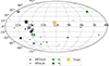 |
Fig. 1. Sky map indicating the positions of the pulsars (stars) and the CGW positions. The size of the pulsar position markers is inversely proportional to the residual root mean square of each pulsar. |
The remaining CGW parameters were chosen considering (a) that the combination of fGW and log10ℳc allowed this frequency evolution, that the transition from unresolved PTs to resolved PTs is realisable using reasonable pulsar distances, and (b) that the S/N of the injected signal, following the definition from Zhu et al. (2016),
![Mathematical equation: $$ \begin{aligned} \rho ^2 = \sum _{j = 1}^{N_{\rm PSR}} \rho _j^2 = \sum _{j = 1}^{N_{\rm PSR}} \sum _{i = 1}^{N_{\rm ToA}} \left[\frac{s(t_i)}{\sigma _j}\right], \end{aligned} $$](/articles/aa/full_html/2026/02/aa55394-25/aa55394-25-eq23.gif) (18)
(18)
falls close to the intermediate (ρ ∼ 30) signal regime, where s(ti) is the injected CGW signal and σj is the mean ToA error of the jth pulsar. As pointed out by Zhu et al. (2016), the strong S/N regime has been ruled out for the Virgo cluster by recent PTA analyses, but it is helpful to test the method.
We found that for the EPTA dataset, these conditions were met for log10ℳc = 9.1 and fGW = 15.9 nHz, corresponding to the sixth frequency bin of the PTA, when we compared pulsars at 1 kpc and 4 kpc distance. This set-up was our fiducial choice of parameters (later: Case (1)), to which we compared other set-ups in order to illustrate other parameter dependences than the pulsar distance. The fGW − log10ℳc parameter space is visualised in Fig. 2, together with the regions for which the PT was resolved, given a timing baseline of 10 yr and two different values of pulsar-CGW angular separation, μ. The fGW-range in which the transition from unresolved to resolved PTs can be tested is clearly reasonably narrow, which illustrates our specific choices of log10ℳc and fGW.
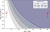 |
Fig. 2. fGW − log10ℳc pfGW − log10ℳc parameter space. The shaded areas indicate the region of resolved PTs for a PTA timing baseline of 10 years. The grey areas correspond to an angular separation between the pulsar and the CGW source of 90°, and the blue areas correspond to 22.5°. The darker and lighter shades refer to a pulsar distance of 1 kpc and 4 kpc, respectively. The red symbols indicate the positions of two exemplary SMBHB candidates in this parameter space, with fGW estimates and upper limits of log10ℳc from electromagnetic models or PTA analyses (OJ287: Titarchuk et al. 2023; Komossa et al. 2023, 3C66B: Cardinal Tremblay et al. 2025). |
To aid comparability across all our simulations, we henceforth fixed the scheme of nearby pulsars sitting at a distance of 1 kpc and distant pulsars that were placed at a distance of 4 kpc. This left the parameters dL and log10ℳc to regulate the frequency evolution, strain amplitude, and S/N of the injected signal.
We assumed that the pulsars at 4 kpc had similar ToA uncertainties as the pulsars at 1 kpc. Although this is counter-intuitive following the well-known scaling between the ToA uncertainty and S/N, which is intimately linked to the pulsar distance, we argue that in light of the FAST radio telescope or the Square Kilometre Array, it is reasonable to assume that pulsars at moderately larger distances (e.g. 4 kpc) yield similar ToA uncertainties as those obtained from observations with current radio telescopes. With the larger observational frequency bandwidths and better telescope gains of these next-generation facilities, the timing precision of most PTA sources are limited by jitter and not by sensitivity. For example, this can be achieved by adapting the integration time, that is, weaker pulsars are observed longer, a strategy that is for instance used in the current scheduling of the MeerKAT PTA (Miles et al. 2022; Middleton et al. 2025).
To explore different regimes of CGW strain and to constrain the effect of the PT resolution, we analysed a total of three different CGW injection cases:
-
Case (1): resolved PTs for dp = 4 kpc; log10ℳc = 9.1; dL = 15 Mpc; h0, (1) = 9.9 × 10⁻¹⁵; S/N ∼ 36
-
Case (2): resolved PTs for dp = {1 kpc, 4 kpc}; log10ℳc = 9.5; dL = 70 Mpc; h0, (2) = h0, (1); S/N ∼ 36
-
Case (3): resolved PTs for dp = 4 kpc, log10ℳc = 9.1; dL = 3 Mpc; h0, (3) = 5h0, (1); S/N ∼ 181.
The particular choices of dL and log10ℳc enabled the following tests: By comparing Cases (1) and (2), we investigated whether changing to resolved PTs yielded a singular improvement of the CGW analysis method or if any improvement increases with a larger frequency difference between ET and PTs, while maintaining the same S/N in both cases. On the other hand, the comparison of Cases (1) and (3) shows the effect that a higher S/N has on any improvement effect, while maintaining the same frequency evolution of the source.
We note that due to the angular proximity to the fiducial CGW position of some pulsars in the EPTA dataset, even at 4 kpc, their PTs are not resolved. In order to single out the effect of a resolved PT, we restricted ourselves to using only 20 out of the 25 EPTA pulsars, for which the PTs are fully resolved at a mean pulsar distance of 4 kpc. Speri et al. (2023) demonstrated that for the latest IPTA dataset (IPTA DR2) and for the EPTA dataset (EPTA DR2), ∼95% of the recovered S/N of the GW signal can be recovered using the most responsive ∼20 pulsars of these datasets. The assumption of a 20-pulsar PTA is therefore sufficiently realistic. We refer to this subset as the EPTA20 dataset. The resulting pulsar sky distribution is shown in Fig. 1, where the size of the markers is inversely proportional to the residual root mean square of each pulsar.
Similar to Zhu et al. (2016), we analysed 500 realisations of the datasets. The analysis methods relevant for the respective section are described at the beginning of each section.
3. Bayesian CGW search
It is common amongst the PTA community to constrain the posterior distributions of PTA parameters in a Bayesian approach by sampling the PTA likelihood function (van Haasteren et al. 2009; van Haasteren & Levin 2013),
 (19)
(19)
In sampling the PTA likelihood function, Eq. (19), the posterior distribution of the CGW parameters log10fGW, log10ℳc, log10h, ϕGW, cos θGW, cos ι, Φ(t), and ψ are determined. When the PT is not considered in the model, the chirp mass cannot be constrained. We employed the analysis scheme that is most commonly used in the PTA community, (e.g. Falxa et al. 2023; EPTA Collaboration and InPTA Collaboration 2023; Agazie et al. 2023; Reardon et al. 2023), namely a Markov chain Monte Carlo (MCMC) sampler, PTMCMC (Ellis & van Haasteren 2017), and the ENTERPRISE software (Ellis et al. 2020) to build the PTA model and calculate the likelihood.
3.1. Results for the test-case scenario
In this part, we aim to investigate whether resolved PTs can lead to improved posteriors of an ET-only MCMC search compared unresolved PTs. In order to keep the PTA dataset as realistic as possible, we analysed the EPTA20 dataset as described above, once with pulsars at 1 kpc, and once with pulsars at 4 kpc. Real PTA datasets are not only affected by WN, but also by RN. As RN processes are known to be covariant with GW parameters, we tested the effect of additional RN in the dataset on the outcome of our simulation. Thus, we started by analysing the Case (1) simulation, once in a dataset with WN only, and once in a dataset with RN also present in each pulsar ToA series. For the simulations, we randomly chose the RN amplitude and spectral index for each pulsar from log10ARN ∈ [ − 15.5, −13.5] and γ ∈ [1.7, 2.2]. The resulting corner plots from analysing 500 realisations of each setup are shown in Fig. 3.
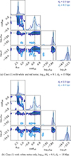 |
Fig. 3. Corner plot of the CGW parameter posteriors (excluding log10ℳc, Φ0, ψ) created from the joint MCMC chain of 500 realisations of each dataset. It shows the result from the dataset containing a CGW signal with log10ℳc = 9.1. The darker contours correspond to the PTA with pulsars at 1 kpc, and the lighter contours correspond to the PTA with pulsars at 4 kpc. |
We found, first, that in both analyses, the marginalised CGW parameter posteriors obtained from the 4 kpc-PTAs (i.e. with resolved PTs) were either narrower and/or more accurate. This held not only for the source position parameter distributions, cos θGW and ϕGW, but also for the posteriors of the GW strain, log10h, and the GW frequency, log10fGW.
The posterior of the GW frequency exhibits an interesting behaviour for the 4 kpc-set-up. Next to the dominant peak, exactly at the ET frequency, it featured a second smaller peak at a slightly lower frequency. Comparing its position to the distribution of PT frequencies in the PTA setup, we found that it coincides very well. We therefore assumed that this additional peak was likely caused by an occasional confusion of the ET frequency with the PT frequency during the MCMC sampling. The ET-only search tried to fit a single sinusoidal pattern with a frequency commonly found in all pulsars, which predominantly is the case at the ET frequency. For the random noise fluctuations present in all pulsars, some correlation can be picked up by chance at the PT frequencies as well, however. This apparent correlation is only a coincidence, unlike the actually correlated signal at the ET frequency. Nonetheless, it causes the MCMC chain to stray into that area of the parameter space. This forms the second peak, but the peak around the ET is more significant. At the same time, this allowed us to understand why the same posterior of the 1 kpc set-up was broader at the position of the injected CGW frequency. Here, the PTs and the ET are not resolved, and the occasional confusion of the MCMC chain into the PT frequencies therefore becomes visible as a broadened posterior distribution.
Additionally, we demonstrated that the WN-only simulation produces representative results of the more realistic WN+RN simulation. This is expected because fGW = 15.9 nHz is the higher-frequency regime of a PTA dataset, in which the effect of RN is weaker. To reduce the complexity of the set-up and separate the PT effect, we therefore restricted ourselves to the more simplistic WN-only simulations.
In the next step, we studied the behaviour of this effect using the Case (2) and Case (3) CGW injections, again for the EPTA20 pulsars at either 1 kpc or 4 kpc. The resulting corner plots of the CGW parameter posteriors are shown in Fig. 4.
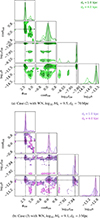 |
Fig. 4. Corner plot of the CGW parameter posteriors (excluding log10ℳc, Φ0, ψ) created from the joint MCMC chain of 500 realisations of each dataset. The darker contours correspond to the PTA with pulsars at 1 kpc, and the lighter contours correspond to the PTA with pulsars at 4 kpc. |
In Case (2), the PTs were resolved for both pulsar distances. Clearly, the marginalised posteriors of the individual parameters show no significant improvements at a larger distance. The only notable difference in the posteriors of Case (2) is found in the distribution of log10fGW. This shows that the analysis performance cannot be amplified by a PT separation of multiple frequency bins compared to a small separation by a single frequency bin. We therefore conclude that for the Bayesian analysis, there is only a single improvement step, which is caused by the transition from unresolved to resolved PTs.
With Case (3), we demonstrate that the improvement achieved with larger pulsar distances is similarly visible for an increased source strain. Notably, the secondary peak in the posterior of log10fGW became slightly larger. This is expected because the larger signal strength amplifies the side effect that the MCMC chain occasionally samples the PT frequencies.
Combining above findings across all three cases, the analysis demonstrates that the observed enhancement effect is caused by the transition from unresolved to resolved PTs.
3.2. PTA set-up and source position
In general, whether it is possible to constrain the parameters of a CGW signal present in a PTA dataset depends on a wide range of characteristic properties of the PTA dataset, such as the number of pulsars, their noise properties, and the overall S/N of the signal, as well as the individual S/N contributions of the pulsars.
We demonstrated that with a sufficient S/N of the signal, resolved PTs can improve the parameter recovery of a Bayesian ET-only CGW analysis. Two main factors set a natural limit to this effect: the distribution of pulsars on the sky, and their individual S/N contribution to the CGW detection in the PTA. Eq. (15) shows that the PT frequency difference does not only depend on the pulsar distance, but also on their location with respect to the CGW source. If the pulsars are too close to the source,  , and so ωa ∼ ωE, even for large da. In this case, even pulsars at large distances have unresolved PTs. On the other hand, when the source is located at a greater angular distance to some of the pulsars, but their S/N contribution is not significant, there is no visible improvement of the posteriors because their behaviour is dominated by the higher S/N pulsars.
We tested these limiting cases by changing the source position from the Virgo cluster to two other positions, P1 = (RA 18 h, Dec −22.5 deg) and P2 = (RA 3 h, Dec −45 deg). P1 resembles a location in the vicinity of the majority of pulsars, whereas P2 is at a larger distance to pulsars with a large RMS. For each of the three cases, the distribution of the PT frequency versus the S/N of the signal in each pulsar is shown in Fig. 5. For these calculations, we used the Case (1) set-up.
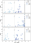 |
Fig. 5. Distribution of PT frequencies vs. S/N contribution in the EPTA20 dataset for three different CGW source positions and pulsars at 1 kpc (dark blue squares) and 4 kpc (light blue dots). The CGW frequency (ET frequency) is indicated as the vertical dark blue line. The fundamental frequencies of the PTA with Tobs = 10 yr are indicated with the vertical grey lines and labels. Top: Virgo cluster. Middle: P1 = (RA 18 h, Dec −22.5 deg). Bottom: P2 = (RA 3 h, Dec −45 deg). Due to the dependence of the strain on the angular distance between the pulsar and the source (cf. Eq. (5)), the S/N varies across the three positions. |
Evidently, the improvement strongly depends on the pulsar constellation. While for a CGW at (and around) P1, the S/N of the signal is high and promises a certain detection, only a few pulsars have resolved PTs at 4 kpc, and they only carry a marginal fraction of the S/N. For P2, most of the PTs are resolved at the larger pulsar distance, but the overall S/N of the signal is very low due to the change in the angular distance between the pulsars and the CGW source (see Eq. (5)). In this case, we therefore expect that the improvement is significantly impaired by the poor detectability of the signal and that it is therefore likely not evident. In comparison, we found for the source position close to the Virgo cluster sky position that most of the PTs are resolved at 4 kpc and that the S/N is sufficiently large. Thus, the effect is visible.
3.3. Adding pulsars to an existing PTA
The way we investigated the behaviour of the Bayesian analysis method in the previous subsections corresponds to analysing only a subset of more distant pulsars in a PTA dataset. Actual PTA datasets span multiple decades, and some of the most precisely timed pulsars also lie at a comparably small distance to Earth. Moreover, in the current state, PTA datasets only contain a limited number of pulsars, and it is therefore not feasible to form meaningful subsets in the near future. It is therefore more realistic to investigate the effect of adding pulsars at a greater distance on the Bayesian parameter recovery of a CGW signal. We tested this by adding 20 pulsars to the EPTA20 dataset, which are shown as grey stars in Fig. 1. The .par-files of the new pulsars were taken from the published MPTA and PPTA datasets (Miles et al. 2024; Reardon et al. 2023), and we therefore refer to them as the IPTA20 dataset. The EPTA20 pulsars are placed at 1 kpc distance, and the added IPTA20 pulsars are located at a distance of ∼4 kpc. As any addition of pulsars to a dataset increases the S/N of the CGW, we investigated two scenarios: (a) the added pulsars increase the S/N of the signal by ∼15%, and (b) the added pulsars increase the S/N by ∼60%. The difference in the S/N was achieved by choosing the RMS of the added pulsars accordingly; a larger RMS means a lower sensitivity. The corner plot of the posterior distribution for the latter scenario (60% S/N increase) is shown in Fig. 6. In both scenarios, we found that the larger dataset provided a better position recovery and a more accurate strain recovery. On the other hand, the recovery of fGW was still slightly impaired due to the significant contribution from the close-by pulsars. Comparing the two scenarios, we found overall that if the more distant pulsars contribute a similar or slightly lower S/N than the close-by pulsars, they still improve the parameter recovery.
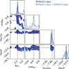 |
Fig. 6. Bayesian posteriors for 500 realisations of the Case (1) injection. The darker contours correspond to the EPTA20 dataset, and the lighter contours show the EPTA20+IPTA20 dataset, which has an S/N increase of 40%. |
3.4. Bias in the source position recovery
As indicated by previous studies such as Zhu et al. (2016), we found that biases of parameter recoveries such as the CGW source position are closely linked to the confusion between the ET and PTs that is unaccounted for in an ET-only search. We demonstrate that an ET-only search with resolved pulsar terms is similarly capable of removing the position recovery bias as including the PTs in the search using our miniature toy-model PTA. To this end, we injected a CGW with a high S/N (log10ℳc = 9.0, dL = 15 Mpc) into four pulsars placed in the Galactic plane, with an RMS of 100 ns. These four pulsars sufficiently recreated the setup from Zhu et al. (2016) because their dataset was also dominated by this small number of pulsars with a high ToA precision. The resulting maximum likelihood values for the CGW source position obtained from 50 exemplary realisations of each dataset are shown in Fig. 7.
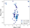 |
Fig. 7. Maximum likelihood solutions for the CGW position parameters ϕGW and θGW (given in radians) using 50 realisations of a CGW signal injected to the 4PSR-GALACTIC dataset with pulsars at a mean distance of |


The source positions recovered using the realisations of the 1 kpc dataset exhibit a similar offset to the injected source position, as shown in Fig. 1 in Zhu et al. (2016). The slight differences between the distribution of our results and those by Zhu et al. (2016) are caused by the different analysis methods: We presented the maximum likelihood solutions obtained from a Bayesian sampling analysis, while Zhu et al. (2016) used a frequentist method.
Using the more distant dataset, we demonstrate that improving the source recovery is not only possible by including the PTs, as indicated by Zhu et al. (2016). It is similarly achievable by using good pulsars at a larger distance, such that the PTs become resolved.
4. Variance in the per-frequency optimal statistic
A computationally efficient way to determine the presence of an HD correlation in a PTA dataset is the frequentist optimal statistic (OS) Anholm et al. (2009), Demorest et al. (2013), Chamberlin et al. (2015), Vigeland et al. (2018). Recently, Gersbach et al. (2025) generalised this framework to the so-called per-frequency optimal statistic (PFOS), which allowed us to characterise the spectral shape of a GW signal present in the PTA dataset by determining the HD content in each frequency bin individually. Gersbach et al. (2025) specifically showed that this method is also capable of indicating the presence of HD-correlated signals limited to a few bins or a single-frequency bin, such as a CGW. These narrow-band signals manifest in terms of significantly larger PSD estimators at these specific frequencies compared to the PSD estimators at other frequencies.
While the OS analysis framework per se is not the optimal way to detect a deterministic signal such as a CGW (this would rather be a matched filter, e.g. the ℱe or ℱp statistic Babak & Sesana 2012), the ETs of the CGW signal exhibit an HD correlation (Romano & Allen 2024) that can be visible in an OS spectrum calculated using the PFOS. The OS analysis is typically employed as a first step in a PTA data analysis because it is much faster and less computationally costly than a full Bayesian analysis of the dataset, especially in light of ever growing datasets. Thus, it is interesting to explore the behaviour of this statistic in the presence of a CGW signal and varying pulsar distances.
4.1. Analysis procedure
The calculation of the PFOS required calculating the PTA free spectrum, that is, determining the amplitudes of the individual Fourier components of the cross-correlation matrix, Eq. (2). The signal of a detectable circular binary manifests itself as a stand-out peak in a single bin of this free spectrum. The free spectrum does not yield any information about the spatial correlation of the signal, however. In Fig. 8 we present the free spectrum of a dataset containing a single CGW signal at 22.3 nHz and an uncorrelated single-bin red-noise signal at 11.2 nHz (both frequencies are multiples of 1/Tobs). Both create a peak in the free spectrum, but only one originates from a CGW.
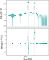 |
Fig. 8. Comparison between a free spectrum and optimal statistic analysis at hand of a simulated dataset with an injection of a CGW and a single bin uncorrelated CRN. Upper plot: Free spectrum. Lower plot: Per-frequency OS. |
Under the assumption that the dataset only contains a GW signal in a few of its frequency bins, it can be analysed with the narrow-band PFOS (Gersbach et al. 2025). Neglecting the pulsar pair covariance, that is, the off-diagonal entries in Cab, cd in Gersbach et al. (2025), we derived the estimator for the GW PSD at the kth frequency bin with the GW frequency fk,
 (20)
(20)
where ρab(fk) and σab(fk) denote the pulsar pair correlations and their uncertainties as given by Eqs. (33) and (34) in Gersbach et al. (2025).
As shown in the lower plot of Fig. 8, this PFOS evaluation now allowed us to identify the CGW as a narrow-band HD correlated signal, while the uncorrelated signal is not visible in the PFOS spectrum.
Across all evaluated frequency bins, the measured PFOS values depend on the specific realisation of the noise processes making up the analysed dataset. Thus, when creating a series of dataset realisations using the same noise parameters, the resulting PFOS values vary, and the spread across all realisations indicates the reliability of the estimator.
As shown by Allen (2023), the PT leads to an increase in the variance in the HD correlation. In a PFOS analysis, we therefore expect it to act like the uncorrelated narrow-band noise in Fig. 8, increasing the uncertainty of the estimator and subsequently leading to a larger spread in the estimators across multiple dataset realisations in the bins closest to the PT frequencies. In the dataset of nearby pulsars, the ET and PT frequencies fall into the same frequency bin, meaning that the PT blurs the information content of the ET. In a dataset with resolved ET and PTs, we expect, on the other hand, that the separation clears the ET frequency bin from the PT noise, which in return should lead to a measurable decrease in the variation of the PFOS value in the ET bin.
4.2. Results from the EPTA-like dataset
The results of the PFOS analyses for the 500 realisations of the EPTA20 datasets with each of the three CGW signals described in Sect. 2.3 are shown in Fig. 9. The violin plots resemble the distribution of P(f) estimates from each realisation. The comparisons demonstrate that the variation in the ET bin diminishes notably in a dataset that consists of pulsars that lie farther away.
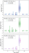 |
Fig. 9. Distribution of narrow-band PFOS values for 500 realisations of the EPTA20 PTA dataset at different average pulsar distances. Each point shows the PFOS estimator of the power spectrum amplitude at the respective frequency for a single dataset realisation. From top to bottom: Cases (1)–(3), as described in Sect. 2.3. |
For both simulations with log10ℳc = 9.1, we clearly find that the spread between the realisations decreases as the ET and PT become resolved. This effect is more pronounced for a higher CGW strain (Case 3). Simultaneously, we note that the spread across the realisations increases in the adjacent lower frequency bin. This is testament to the noise-like treatment of the PT. As the ET falls together with the PT, the latter adds noise to the signal in the corresponding frequency bin. With increasing separation between the two, however, the noise shifts towards the lower frequency bin and only leaves the signal in the ET frequency bin. Unsurprisingly, the spread in the OS values of the simulations using log10ℳc = 9.5 (Case 2) does not differ significantly for the two mean pulsar distances. As discussed previously, for log10ℳc = 9.5, the ET and PT are resolved in all pulsars already for  kpc, and the further separation of the PTs from the ET does not improve the PFOS S/N in the ET frequency bin.
Overall, we deduce from the results of the two PTA set-ups that the identification of narrow-band HD correlations from CGW signals using the PFOS method benefits from separating the ET and PT frequencies by moving to more distant pulsars. This can be of special interest for lower GW strains, that is, for sources at the detection limit: The CGW would be more reliably visible as a raised P(f) value in the PFOS spectrum for pulsars at a large distance to the Earth, while a larger spread for closer pulsars would mean that the P(f) is more likely to vanish in the noise floor of the data.
5. Conclusions and outlook
We have shown that including pulsars at a larger distance to the Earth can improve the performance of two PTA CGW analysis tools in the presence of a high-frequency (≳10 nHz) CGW signal within the respective dataset through the separation of the ET and the PT.
The Bayesian likelihood search using an ET-only CGW model improves using pulsars at a greater distance. Especially the posterior distributions of the source position parameters, the GW frequency, and the strain become more constrained. We tested this effect using an idealised scenario with pulsars either nearby or farther away, but we also demonstrated that adding more distant pulsars to an existing array improves the capabilities of the PTA to constrain CGW parameters in an ET-only search.
Our analyses demonstrated that the improvement of this technique is highly dependent on the constellation of pulsars with respect to the CGW source position, as well as on the S/N with which the signal appears in the residuals of each pulsar. While we did not verify this implicitly for the frequentist analysis, they behave similarly, so that it is safe to assume that it applies to both techniques.
The frequentist analysis with the narrow-band optimal statistic (Gersbach et al. 2025) more reliably indicates the excess power in the regarding frequency bins close to the GW frequency when it is applied to pulsars with resolved PTs. This effect is especially noteworthy for weaker GW sources, where the CGW is close to the noise floor of the timing residuals. In the (currently unrealistic) case that the CGW strain is significantly above the noise floor, this separation effect proves not as relevant for the performance of the PFOS because the CGW is always visible.
Overall, we explored an alternative approach to remedy the impairment in CGW search and analysis techniques in the light of unconstrained PTs due to imprecisely known pulsar distances. We demonstrated that parameter mis-specifications and loss of S/N can be diminished by using pulsars with resolved PTs.
The findings of this work also have several subsequent implications. The notable improvement that a group of pulsars with fully resolved PTs can provide suggests that it might be interesting for the analysis of a future PTA dataset with 𝒪(100 + ) pulsars to perform a CGW search on only a subset of pulsars at a larger distance. This might involve improving the detection of a high-frequency source using the PFOS, or improving the constraints on the parameters of a CGW when one is detected. Additionally, the location of the example SMBHB candidates in Fig. 2 indicates that there are some high-frequency candidates for which an ET-only targeted search is likely sufficient, whereas others with a predicted fGW of only a few nano-Hertz should be targeted with a full ET+PT model. Furthermore, the behaviour of the GW frequency posterior (see Fig. 4), namely that it sometimes breaks out to the PT frequencies, might be used to constrain the frequency evolution of the CGW without the need of precisely known pulsar distances.
Acknowledgments
We thank Mikel Falxa and Stanislav Babak for the fruitful discussions and comments on CGW modelling and the Optimal Statistic. All authors affiliated with the Max-Planck-Gesellschaft (MPG) acknowledge its constant support. KG acknowledges support from the International Max Planck Research School (IMPRS) for Astronomy and Astrophysics at the Universities of Bonn and Cologne and the Bonn-Cologne Graduate School of Physics and Astronomy. NP’s contribution to the study was partially conducted under the state assignment of Lomonosov Moscow State University. The analysis done in this publication made use of the open source pulsar analysis packages TEMPO2 (Hobbs et al. 2006), LIBSTEMPO (Vallisneri 2020), ENTERPRISE (Ellis et al. 2020) and ENTERPRISE_EXTENSIONS (Taylor et al. 2021), as well as open source PYTHON libraries including Numpy (Harris et al. 2020), Matplotlib (Hunter 2007), Astropy (Astropy Collaboration 2013, 2018, 2022) and Chainconsumer (Hinton 2016).
References
- Agazie, G., Anumarlapudi, A., Archibald, A. M., et al. 2023, ApJ, 951, L8 [NASA ADS] [CrossRef] [Google Scholar]
- Allen, B. 2023, Phys. Rev. D, 107, 043018 [NASA ADS] [CrossRef] [Google Scholar]
- Allen, B., & Romano, J. D. 1999, Phys. Rev. D, 59, 102001 [NASA ADS] [CrossRef] [Google Scholar]
- Anholm, M., Ballmer, S., Creighton, J. D. E., Price, L. R., & Siemens, X. 2009, Phys. Rev. D, 79, 084030 [NASA ADS] [CrossRef] [Google Scholar]
- Arzoumanian, Z., Brazier, A., Burke-Spolaor, S., et al. 2014, ApJ, 794, 141 [NASA ADS] [CrossRef] [Google Scholar]
- Astropy Collaboration (Robitaille, T. P., et al.) 2013, A&A, 558, A33 [NASA ADS] [CrossRef] [EDP Sciences] [Google Scholar]
- Astropy Collaboration (Price-Whelan, A. M., et al.) 2018, AJ, 156, 123 [Google Scholar]
- Astropy Collaboration (Price-Whelan, A. M., et al.) 2022, ApJ, 935, 167 [NASA ADS] [CrossRef] [Google Scholar]
- Babak, S., & Sesana, A. 2012, Phys. Rev. D, 85, 044034 [NASA ADS] [CrossRef] [Google Scholar]
- Babak, S., Petiteau, A., Sesana, A., et al. 2016, MNRAS, 455, 1665 [NASA ADS] [CrossRef] [Google Scholar]
- Babak, S., Falxa, M., Franciolini, G., & Pieroni, M. 2024, Phys. Rev. D, 110, 063022 [Google Scholar]
- Bailes, M., Berger, B. K., Brady, P. R., et al. 2021, Nat. Rev. Phys., 3, 344 [NASA ADS] [CrossRef] [Google Scholar]
- Begelman, M. C., Blandford, R. D., & Rees, M. J. 1980, Nature, 287, 307 [Google Scholar]
- Burke-Spolaor, S. 2015, ArXiv e-prints [arXiv:1511.07869] [Google Scholar]
- Cardinal Tremblay, J., Goncharov, B., van Haasteren, R., et al. 2025, ArXiv e-prints [arXiv:2508.20007] [Google Scholar]
- Chamberlin, S. J., Creighton, J. D. E., Siemens, X., et al. 2015, Phys. Rev. D, 91, 044048 [NASA ADS] [CrossRef] [Google Scholar]
- Chen, J.-W., & Wang, Y. 2022, ApJ, 929, 168 [Google Scholar]
- Corbin, V., & Cornish, N. J. 2010, ArXiv e-prints [arXiv:1008.1782] [Google Scholar]
- Deller, A. T., Brisken, W. F., Chatterjee, S., et al. 2011, in 20th Meeting of the European VLBI Group for Geodesy and Astronomy, eds. W. Alef, S. Bernhart, & A. Nothnagel, 178 [Google Scholar]
- Demorest, P. B., Ferdman, R. D., Gonzalez, M. E., et al. 2013, ApJ, 762, 94 [Google Scholar]
- Detweiler, S. 1979, ApJ, 234, 1100 [NASA ADS] [CrossRef] [Google Scholar]
- Ellis, J., & van Haasteren, R. 2017, https://doi.org/10.5281/zenodo.1037579 [Google Scholar]
- Ellis, J. A., Jenet, F. A., & McLaughlin, M. A. 2012, ApJ, 753, 96 [NASA ADS] [CrossRef] [Google Scholar]
- Ellis, J. A., Vallisneri, M., Taylor, S. R., & Baker, P. T. 2020, https://doi.org/10.5281/zenodo.4059815 [Google Scholar]
- EPTA Collaboration and InPTA Collaboration (Antoniadis, J., et al.) 2023, A&A, 678, A50 [CrossRef] [EDP Sciences] [Google Scholar]
- EPTA Collaboration (Antoniadis, J., et al.) 2023, A&A, 678, A48 [Google Scholar]
- Estabrook, F. B., & Wahlquist, H. D. 1978, Acta Astron., 5, 5 [Google Scholar]
- Falxa, M., Babak, S., Baker, P. T., et al. 2023, MNRAS, 521, 5077 [NASA ADS] [CrossRef] [Google Scholar]
- Foster, R. S., & Backer, D. C. 1990, ApJ, 361, 300 [NASA ADS] [CrossRef] [Google Scholar]
- Gair, J., Romano, J. D., Taylor, S., & Mingarelli, C. M. F. 2014, Phys. Rev. D, 90, 082001 [NASA ADS] [CrossRef] [Google Scholar]
- Gersbach, K. A., Taylor, S. R., Meyers, P. M., & Romano, J. D. 2025, Phys. Rev. D, 111, 023027 [Google Scholar]
- Harris, C. R., Millman, K. J., van der Walt, S. J., et al. 2020, Nature, 585, 357 [NASA ADS] [CrossRef] [Google Scholar]
- Hellings, R. W., & Downs, G. S. 1983, ApJ, 265, L39 [NASA ADS] [CrossRef] [Google Scholar]
- Hinton, S. R. 2016, J. Open Source Softw., 1, 00045 [NASA ADS] [CrossRef] [Google Scholar]
- Hobbs, G. B., Edwards, R. T., & Manchester, R. N. 2006, MNRAS, 369, 655 [Google Scholar]
- Hunter, J. D. 2007, Comput. Sci. Eng., 9, 90 [NASA ADS] [CrossRef] [Google Scholar]
- Jaffe, A. H., & Backer, D. C. 2003, ApJ, 583, 616 [NASA ADS] [CrossRef] [Google Scholar]
- Kato, R., & Takahashi, K. 2023, Phys. Rev. D, 108, 123535 [Google Scholar]
- Komossa, S., Grupe, D., Kraus, A., et al. 2023, MNRAS, 522, L84 [NASA ADS] [CrossRef] [Google Scholar]
- Kormendy, J., & Richstone, D. 1995, ARA&A, 33, 581 [Google Scholar]
- Lee, K. J., Wex, N., Kramer, M., et al. 2011, MNRAS, 414, 3251 [CrossRef] [Google Scholar]
- Lentati, L., Alexander, P., Hobson, M. P., et al. 2014, MNRAS, 437, 3004 [NASA ADS] [CrossRef] [Google Scholar]
- Lorimer, D. R., & Kramer, M. 2005, Handbook of Pulsar Astronomy (Cambridge: Cambridge University Press) [Google Scholar]
- Maggiore, M. 2000, Phys. Rep., 331, 283 [Google Scholar]
- Manchester, R. N., & IPTA 2013, Class. Quant. Grav., 30, 224010 [Google Scholar]
- Middleton, H., Shannon, R. M., Bailes, M., et al. 2025, MNRAS, 540, 603 [Google Scholar]
- Miles, M. T., Shannon, R. M., Bailes, M., et al. 2022, MNRAS, 519, 3976 [Google Scholar]
- Miles, M. T., Shannon, R. M., Reardon, D. J., et al. 2024, MNRAS, 536, 1467 [Google Scholar]
- Milosavljević, M., & Merritt, D. 2001, ApJ, 563, 34 [Google Scholar]
- Mingarelli, C. M. F., Grover, K., Sidery, T., Smith, R. J. E., & Vecchio, A. 2012, Phys. Rev. Lett., 109, 081104 [Google Scholar]
- Mingarelli, C. M. F., Anderson, L., Bedell, M., Spergel, D. N., & Moran, A. 2018, ArXiv e-prints [arXiv:1812.06262] [Google Scholar]
- Petiteau, A., Babak, S., Sesana, A., & de Araújo, M. 2013, Phys. Rev. D, 87, 064036 [NASA ADS] [CrossRef] [Google Scholar]
- Petrov, P., Schult, L., Taylor, S. R., et al. 2025, ArXiv e-prints [arXiv:2510.01316] [Google Scholar]
- Phinney, E. S. 2001, ArXiv e-prints [arXiv:astro-ph/0108028] [Google Scholar]
- Rajagopal, M., & Romani, R. W. 1995, ApJ, 446, 543 [NASA ADS] [CrossRef] [Google Scholar]
- Ravi, V., Wyithe, J. S. B., Hobbs, G., et al. 2012, ApJ, 761, 84 [NASA ADS] [CrossRef] [Google Scholar]
- Reardon, D. J., Zic, A., Shannon, R. M., et al. 2023, ApJ, 951, L6 [NASA ADS] [CrossRef] [Google Scholar]
- Romano, J. D., & Allen, B. 2024, Class. Quant. Grav., 41, 175008 [NASA ADS] [CrossRef] [Google Scholar]
- Rosado, P. A., Sesana, A., & Gair, J. 2015, MNRAS, 451, 2417 [NASA ADS] [CrossRef] [Google Scholar]
- Sazhin, M. V. 1978, Soviet Astron., 22, 36 [NASA ADS] [Google Scholar]
- Sesana, A., & Vecchio, A. 2010, Phys. Rev. D, 81, 104008 [NASA ADS] [CrossRef] [Google Scholar]
- Sesana, A., Haardt, F., Madau, P., & Volonteri, M. 2004, ApJ, 611, 623 [NASA ADS] [CrossRef] [Google Scholar]
- Sesana, A., Vecchio, A., & Volonteri, M. 2009, MNRAS, 394, 2255 [NASA ADS] [CrossRef] [Google Scholar]
- Simon, J., Polin, A., Lommen, A., et al. 2014, ApJ, 784, 60 [Google Scholar]
- Speri, L., Porayko, N. K., Falxa, M., et al. 2023, MNRAS, 518, 1802 [Google Scholar]
- Spiewak, R., Bailes, M., Miles, M. T., et al. 2022, PASA, 39, e027 [NASA ADS] [CrossRef] [Google Scholar]
- Taylor, S., Ellis, J., & Gair, J. 2014, Phys. Rev. D, 90, 104028 [Google Scholar]
- Taylor, S. R., Baker, P. T., Hazboun, J. S., Simon, J., & Vigeland, S. J. 2021, enterprise_extensions, v2.4.3 [Google Scholar]
- Titarchuk, L., Seifina, E., & Shrader, C. 2023, A&A, 671, A159 [NASA ADS] [CrossRef] [EDP Sciences] [Google Scholar]
- Vallisneri, M. 2020, Astrophysics Source Code Library [record ascl:2002.017] [Google Scholar]
- van Haasteren, R., & Levin, Y. 2013, MNRAS, 428, 1147 [NASA ADS] [CrossRef] [Google Scholar]
- van Haasteren, R., Levin, Y., McDonald, P., & Lu, T. 2009, MNRAS, 395, 1005 [NASA ADS] [CrossRef] [Google Scholar]
- Vigeland, S. J., Islo, K., Taylor, S. R., & Ellis, J. A. 2018, Phys. Rev. D, 98, 044003 [NASA ADS] [CrossRef] [Google Scholar]
- Wang, Y., & Mohanty, S. D. 2017, Phys. Rev. Lett., 118, 151104 [NASA ADS] [CrossRef] [Google Scholar]
- Xu, H., Chen, S., Guo, Y., et al. 2023, RAA, 23, 075024 [NASA ADS] [Google Scholar]
- Zhu, X. J., Wen, L., Xiong, J., et al. 2016, MNRAS, 461, 1317 [Google Scholar]
All Figures
|
Fig. 1. Sky map indicating the positions of the pulsars (stars) and the CGW positions. The size of the pulsar position markers is inversely proportional to the residual root mean square of each pulsar. |
| In the text | |
|
Fig. 2. fGW − log10ℳc pfGW − log10ℳc parameter space. The shaded areas indicate the region of resolved PTs for a PTA timing baseline of 10 years. The grey areas correspond to an angular separation between the pulsar and the CGW source of 90°, and the blue areas correspond to 22.5°. The darker and lighter shades refer to a pulsar distance of 1 kpc and 4 kpc, respectively. The red symbols indicate the positions of two exemplary SMBHB candidates in this parameter space, with fGW estimates and upper limits of log10ℳc from electromagnetic models or PTA analyses (OJ287: Titarchuk et al. 2023; Komossa et al. 2023, 3C66B: Cardinal Tremblay et al. 2025). |
| In the text | |
|
Fig. 3. Corner plot of the CGW parameter posteriors (excluding log10ℳc, Φ0, ψ) created from the joint MCMC chain of 500 realisations of each dataset. It shows the result from the dataset containing a CGW signal with log10ℳc = 9.1. The darker contours correspond to the PTA with pulsars at 1 kpc, and the lighter contours correspond to the PTA with pulsars at 4 kpc. |
| In the text | |
|
Fig. 4. Corner plot of the CGW parameter posteriors (excluding log10ℳc, Φ0, ψ) created from the joint MCMC chain of 500 realisations of each dataset. The darker contours correspond to the PTA with pulsars at 1 kpc, and the lighter contours correspond to the PTA with pulsars at 4 kpc. |
| In the text | |
|
Fig. 5. Distribution of PT frequencies vs. S/N contribution in the EPTA20 dataset for three different CGW source positions and pulsars at 1 kpc (dark blue squares) and 4 kpc (light blue dots). The CGW frequency (ET frequency) is indicated as the vertical dark blue line. The fundamental frequencies of the PTA with Tobs = 10 yr are indicated with the vertical grey lines and labels. Top: Virgo cluster. Middle: P1 = (RA 18 h, Dec −22.5 deg). Bottom: P2 = (RA 3 h, Dec −45 deg). Due to the dependence of the strain on the angular distance between the pulsar and the source (cf. Eq. (5)), the S/N varies across the three positions. |
| In the text | |
|
Fig. 6. Bayesian posteriors for 500 realisations of the Case (1) injection. The darker contours correspond to the EPTA20 dataset, and the lighter contours show the EPTA20+IPTA20 dataset, which has an S/N increase of 40%. |
| In the text | |
|
Fig. 7. Maximum likelihood solutions for the CGW position parameters ϕGW and θGW (given in radians) using 50 realisations of a CGW signal injected to the 4PSR-GALACTIC dataset with pulsars at a mean distance of |
| In the text | |
|
Fig. 8. Comparison between a free spectrum and optimal statistic analysis at hand of a simulated dataset with an injection of a CGW and a single bin uncorrelated CRN. Upper plot: Free spectrum. Lower plot: Per-frequency OS. |
| In the text | |
|
Fig. 9. Distribution of narrow-band PFOS values for 500 realisations of the EPTA20 PTA dataset at different average pulsar distances. Each point shows the PFOS estimator of the power spectrum amplitude at the respective frequency for a single dataset realisation. From top to bottom: Cases (1)–(3), as described in Sect. 2.3. |
| In the text | |
Current usage metrics show cumulative count of Article Views (full-text article views including HTML views, PDF and ePub downloads, according to the available data) and Abstracts Views on Vision4Press platform.
Data correspond to usage on the plateform after 2015. The current usage metrics is available 48-96 hours after online publication and is updated daily on week days.
Initial download of the metrics may take a while.