| Issue |
A&A
Volume 706, February 2026
|
|
|---|---|---|
| Article Number | A380 | |
| Number of page(s) | 17 | |
| Section | Cosmology (including clusters of galaxies) | |
| DOI | https://doi.org/10.1051/0004-6361/202556020 | |
| Published online | 23 February 2026 | |
Growth rate measurements from a joint analysis of the large-scale galaxy clustering in Fourier and configuration space
1
Aix Marseille Univ, CNRS/IN2P3, CPPM Marseille, France
2
IRFU, CEA, Université Paris-Saclay F-91191 Gif-sur-Yvette, France
3
Departament de Física Quántica i Astrofísica, Universitat de Barcelona Martí i Franqués 1 E08028 Barcelona, Spain
4
Institut d’Estudis Espacials de Catalunya (IEEC) 08034 Barcelona, Spain
5
Institut de Ciències del Cosmos (ICCUB), Universitat de Barcelona (UB), c. Martí i Franquès 1 08028 Barcelona, Spain
★ Corresponding author: This email address is being protected from spambots. You need JavaScript enabled to view it.
Received:
18
June
2025
Accepted:
4
December
2025
Abstract
In this work, we test a framework to analyse redshift-space distortions in configuration and Fourier space simultaneously. We tested our methods with the AbacusSummit suite of N-body simulations as well as a more numerous set of approximate EZmocks, and reproduced the sample of luminous red galaxies from the Baryon Oscillation Spectroscopic Survey (BOSS) and its extension (eBOSS). Our clustering models are based on the effective field theory of large-scale structures in a Lagrangian frame, which is used in the latest results from the Dark Energy Spectroscopic Instrument. We performed a template type of analysis, including dilation parameters and the slope parameter from the ShapeFit framework. We find that the joint space inference yields unbiased and robust constraints on simulated datasets that are consistent with the results from individual spaces or previous methods to obtain consensus results. Our joint space analysis on the BOSS+eBOSS LRG sample obtains fσ8 = 0.463 ± 0.052, which is in good agreement with the official 2020 results.
Key words: cosmological parameters / cosmology: observations / dark energy / large-scale structure of Universe
© The Authors 2026
 Open Access article, published by EDP Sciences, under the terms of the Creative Commons Attribution License (https://creativecommons.org/licenses/by/4.0), which permits unrestricted use, distribution, and reproduction in any medium, provided the original work is properly cited.
This article is published in open access under the Subscribe to Open model. This email address is being protected from spambots. You need JavaScript enabled to view it. to support open access publication.
1. Introduction
Over the past decades, the study of the statistical properties of the large-scale structure (LSS) of our Universe has led to major advances in our understanding of the cosmic amounts of dark energy and dark matter as well as the initial conditions that were the origin of such structures. Larger and denser maps of the LSS have been built thanks to the increasing power of multiplex fiber-fed spectroscopic surveys such as the cosmological programs of the Sloan Digital Sky Survey (SDSS; Eisenstein et al. 2011; Blanton et al. 2017) and the Dark Energy Spectroscopic Instrument (DESI; DESI Collaboration 2016a,b, 2022). Such surveys measure millions of high precision galaxy redshifts and span large fractions of our cosmic history. These maps enable estimates of the galaxy two-point functions, such as the power spectrum (in Fourier space) or the correlation function (in configuration space). The shape of such statistical measurements heavily depends on the expansion history of the Universe and on the growth history of initial cosmological perturbations.
The observed two-point functions of a galaxy redshift survey is anisotropic with respect to the line-of-sight (LOS) due to redshift-space distortions (RSD). Such distortions appear when converting redshifts to distances: peculiar velocities modify the observed redshifts in a coherent manner. On large scales, the velocity field is simply a response to the growth of density perturbations. RSD analyses aim to measure such anisotropies in the two-point functions and provide constraints on the logarithmic growth rate of structure f ≡ dlnD(a)/dlna (where D(a) is the growth factor). Measurements of the growth rate of structures are a powerful cosmological probe of gravity and are complementary to measurements of the expansion rate from type-Ia supernovae or baryon acoustic oscillations (BAOs).
Modeling anisotropies on large linear scales (above ∼80 Mpc) is straighforward (Kaiser 1987), but on intermediate to small scales (below ∼50 Mpc) it can be a challenge due to nonlinear clustering and a more complex galaxy-dark-matter connection. Recently, effective field theories of large-scale structures (EFTofLSS; Ivanov 2022) have been able to model intermediate scale two-point clustering in redshift space. Such theories incorporate effective coefficients that depend on small-scale physics, which are then marginalised over.
Traditionally, RSD measurements have been conducted either in configuration space (Bautista et al. 2021; Hou et al. 2021; Tamone et al. 2020) or in Fourier space (Gil-Marín et al. 2020; de Mattia et al. 2020; Neveux et al. 2020). In configuration space, the two-point correlation function, ξ(r), is estimated with pair-counting algorithms. In Fourier space, the power spectrum, P(k), is estimated by placing galaxies on a regular mesh and performing fast Fourier transforms. Both approaches use the same initial dataset and, in principle, should yield the same cosmological results. In practice, however, they differ in their noise properties, on how they are impacted by systematic effects, and on the choice of scales used for inference1. Therefore, Fourier and configuration space results are highly correlated but not identical, so there is a small gain in combining both results into a single consensus result.
Sánchez et al. (2017) proposed a method to compute consensus results between Fourier and configuration space analyses, which works at the level of the parameter posteriors. The method assumes that individual parameter posteriors are Gaussian and also yield Gaussian consensus posteriors. This assumption can be broken with noisier data where posteriors in each individual analysis space are non-Gaussian.
Dumerchat & Bautista (2022) developed an alternative framework to obtain consensus results, which is based on a joint fit of correlation function and power spectrum multipoles and accounts for their covariance at the inference level. Such a methodology can yield non-Gaussian consensus posteriors on the fitted parameters, so it relies on less assumptions than the method by Sánchez et al. (2017). This methodology was tested on BAO measurements of eBOSS LRG data and yielded consistent results with the official analysis.
In this work, we extend the joint configuration and Fourier space analysis by Dumerchat & Bautista (2022) to an RSD analysis. This paper is organized as follows. Section 2 describes the real and synthetic datasets employed in our analysis, followed by a presentation of different consensus methodologies in Sect. 3. The theoretical model of the two-point functions used in our inferences is described in Sect. 4. In Sect. 5 we present the results of the joint RSD analysis on mock data. Results on eBOSS LRG data are discussed in Sect. 6.
2. Dataset
In this section we summarize the datasets used in our RSD analyses. We also describe the synthetic samples employed to validate our methodology.
2.1. The BOSS and eBOSS sample of LRGs
The third and fourth generations of the SDSS contained two major cosmological surveys: the Baryon Oscillation Spectroscopic Survey (BOSS; Dawson et al. 2013) and its extension, eBOSS (Dawson et al. 2016), each program observed for about five years each. The SDSS used the 2.5-meter Sloan Foundation Telescope at Apache Point Observatory (APO; Gunn et al. 2006), which is equipped with a focal plane able to host 1000 optical fibers and two spectrographs covering the 3600–10 400 Å range in wavelengths (Smee et al. 2013). The main goal of BOSS and eBOSS was the measurement of BAO and RSD to constrain cosmological parameters (Alam et al. 2017, 2021). For that, these surveys measured millions of galaxies and quasars over a large range in redshift (0 < z < 4). These samples are publicly available as part of SDSS Data Release 16 (Ahumada et al. 2020).
To apply our framework, we consider the sample of luminous of red galaxies (LRG) from the combination of BOSS and eBOSS redshits over 0.6 < z < 1.0. The full description of the construction of this sample for the purpose of clustering measurements can be found in Ross et al. (2020). This sample is composed of 174 816 eBOSS LRG redshifts over 4242 deg2 and BOSS LRGs over 9493 deg2 over the same redshift range, yielding a total of 377 458 galaxies. Several weights are computed and assigned to each galaxy to correct for spurious density fluctuations originating from target selection, spectroscopic completeness, fiber collisions, among others. The window function of the survey is characterized by a set of unclustered points, the random catalog, containing about 20 times the number of galaxies. This sample of LRG was used to measure BAO and RSD, both in configuration and Fourier space (Bautista et al. 2021; Gil-Marín et al. 2020).
2.2. Synthetic datasets
We employed two types of synthetic datasets in this work: N-body simulations and approximate methods. N-body simulations are fully nonlinear and are a perfect test bench for our theoretical clustering models (Sect. 4). Approximate mocks have less realistic clustering on small-scales but easily reproduce the survey geometry, the density of tracers and make possible the production of thousands of realisations, which are useful to test the statistical properties of our inferences and estimate sample covariance matrices.
2.2.1. N-body simulations:
The ABACUSSUMMITN-body simulation suite (Garrison et al. 2019) contains 25 independent realisations in a periodic cubic box, each covering a volume of 8 h−3 Gpc3. These mocks use the ABACUS code (Garrison et al. 2021) to evolve 69123 matter particles with mass of 2 × 10⁹ h−1 M⊙ from initial conditions set at z = 99 from second-order Lagrangian perturbation theory. Halos are identified from groups of particles using the specialized spherical-overdensity-based halo finder CompaSO (Hadzhiyska et al. 2022). We used the z = 0.8 snapshot to match the redshift range of the LRG sample. The halos were populated with LRGs using a halo occupation distribution model (HOD; Yuan et al. 2023) matching the clustering properties of DESI Early Data Release (DESI Collaboration 2024). To obtain the covariance matrix of the clustering measurements of our N-body simulations, we used a set of 1000 realizations of (2 h−1 Gpc)3 boxes run with the EZMOCK method (Chuang et al. 2015), tuned to match the clustering of the n-body simulations. Note that these EZmocks are different than those described next.
2.2.2. Approximate mocks:
We used 1000 realizations of the LRG eBOSS+BOSS survey geometry generated with the EZMOCK method (Chuang et al. 2015). This approach employs the Zel’dovich approximation to model the density field at a given redshift and populate it with galaxies. The method is computationally efficient and has been specifically calibrated to reproduce the two- and three-point statistics of the galaxy sample, including mildly nonlinear scales. The angular and redshift distributions of the eBOSS LRG sample, combined with the z > 0.6 CMASS sample, were accurately replicated in these mock catalogs. A detailed description of the EZMOCKS LRG samples can be found in Zhao et al. (2021). These mock catalogs were crucial to the analysis, enabling the estimation of error covariance matrices for clustering measurements, the evaluation of systematic observational effects on cosmology, and the assessment of correlations between different methodologies for deriving consensus results. In our analysis, we consider two fiducial cosmologies. Table 1 presents the fiducial cosmology used for DESI and eBOSS.
Cosmological parameters used in eBOSS and DESI mock catalogs.
2.3. Clustering measurements
We used the Yamamoto estimator to estimate the power spectrum multipoles (Yamamoto et al. 2006). These are computed using PYPOWER2. The survey geometry is described by a window function that defines the observed regions and accounts for selection effects. We apply it by directly convolving the model power spectrum with the window function in Fourier space, following Beutler et al. (2019), Beutler & McDonald (2021). The window function is computed with PYPOWER. The correlation function multipoles are estimated using the Landy–Szalay estimator (Landy & Szalay 1993), and are computed using PYCORR3.
3. Methodology for consensus results
In this section we describe our framework to derive consensus results from a joint RSD analysis in Fourier and configuration space. We first introduce the inference algorithms. Second, we remind the basics of the Gaussian approximation method to obtain consensus results. Lastly, we describe our joint analysis in detail.
3.1. Parameter inference
In this work, we are ultimately interested in the inference of the growth rate of structure f, or its combination with the amplitude of linear perturbations σ8, as well as the dilation parameters q⊥, q∥ describing deviations from the assumed fiducial cosmology. These parameters are defined in Sect. 4.
The likelihood function ℒ of observing a data vector given a model obtained from a set of parameters θ can be written as
 (1)
(1)
where Nbins is the dimension of the data vector, Δi(θ)≡di − mi(θ) is the data-model difference in bin i. The  is an estimate of the precision matrix, computed as
  , where
  is an estimate of the data vector covariance matrix and (1 − DH) is a correction factor, described next.
In this work, our data vector is either the correlation function or power spectrum multipoles. In our joint analysis, the data vector is a concatenation of the multipoles from both spaces. Our covariance matrices C are estimated from a set of synthetic datasets (also referred to as mocks hereafter) reproducing our survey geometry and clustering, so accounts for both cosmic variance and shot-noise contributions. From Nmock mock measurements of two-point functions, the sample covariance is simply defined as
 (2)
(2)
where  is the sample average of the data vector over all mocks.
Since we use a finite number of mocks, the correction factor takes the form DH ≡ (Nbins + 1)/(Nmock − 1) to correct for the biased estimate of the precision matrix (Hartlap et al. 2007). Also, each element of  is affected by its own uncertainty which shall be appropriately propagated to the parameter uncertainties. Following Percival et al. (2014), this correction is done by scaling factors given by
 (3)
(3)
 (4)
(4)
where DH is the Hartlap factor defined above, and
 (5)
(5)
 (6)
(6)
The factor m1 is applied directly to the estimated covariance matrix of the parameters for a specific measurement. Conversely, the factor m2 is used to scale the standard deviation of a parameter across a series of mocks. The values of the parameters m1 and m2 of our baseline analysis are given in Table 2 for configuration space (CS), Fourier space (FS) and joint space (JS).
Correction factors used in the three analyses conducted in this study.
We assumed the covariance matrix to be independent of model parameters and it remains fixed during the inference. Therefore, the c term in Eq. (1) is simply an additive constant. We use two approaches for parameter estimation: a frequentist and a Bayesian one.
3.1.1. Frequentist Approach:
Best-fit parameters are determined by minimizing χ2 using a quasi-Newton minimizer implemented in IMINUIT4. Parameter uncertainties are estimated by identifying intervals where χ2 increases by one unit, corresponding to a 68% confidence level. This approach does not assume Gaussianity of the parameter posterior distribution, so uncertainties can be asymmetric.
3.1.2. Bayesian Approach:
The posterior probability distribution of the parameters θ given the observed data d is given by the Bayes’ theorem, P(θ|d) = ℒ(d|θ)P(θ)/P(d), where ℒ is the likelihood from Eq. (1), P(θ) is the prior and P(d) is the evidence. The likelihood is explored using a Markov chain Monte Carlo (MCMC) algorithm, implemented in EMCEE5 (Foreman-Mackey et al. 2013). We run chains in parallel and assess their convergence using the Gelman-Rubin criterion (Gelman & Rubin 1992).
For most test cases, we checked that both approaches give consistent results. The first approach is faster and used to quickly obtain constraints of a small subset of parameters, which can be run on large samples of mocks, while the second one is slower but accurately describes the correlated posterior distributions of all parameters.
We used the DESILIKE6 framework, a public tool developed by the DESI collaboration that integrates theory modeling, observable definitions, likelihood computation, theory emulation, and posterior sampling and profiling. These tools were employed in the main cosmological results from DESI (DESI Collaboration 2025a,b,c; DESI Collaboration 2025d,f).
3.2. Consensus results from the Gaussian approximation method
Sánchez et al. (2017) proposed a method to obtain consensus results from configuration-space (CS) and Fourier-space (FS) analyses. This method combines posteriors distributions of the parameters of interest, assuming they are Gaussian and also yielding Gaussian consensus porsteriors. We refer to this method as the Gaussian approximation (GA) hereafter.
In the case of RSD analysis, the parameters of interest are the normalized growth rate of structures fσ8 and the dilation parameters q⊥, q∥. Each analysis produces its own posterior which is approximated by a three-dimensional Gaussian centered in θ = [fσ8, q∥, q⊥] with a 3 × 3 parameter covariance Cθ. The consensus result is obtained by constructing a 6 × 6 parameter covariance, where the off-diagonal blocks (i.e., the cross-covariance between parameters in CS and FS) are estimated from mock catalogs. The consensus result is given by θGA and its 3 × 3 covariance CθGA.
Furthermore, Bautista et al. (2021) argued that the cross-covariance block obtained from a set of mocks is representative of the ensemble, but not of a particular realisation. An adjustement of these off-diagonal blocks was proposed, based on the uncertainties of the data realisation itself. This technique was used to obtain consensus between configuration and Fourier space analyses as well as between BAO and RSD constraints (each yielding dilation parameters). A full description of the method we use in this work can be found in Bautista et al. (2021).
3.3. Consensus results from a joint space analysis
An alternative to the Gaussian approximation for obtaining consensus results is to perform a joint fit of both configuration-space and Fourier-space two-point functions, using a single set of parameters. The cross-covariance between multipoles in CS and FS is estimated from mock catalogs. We refer to this approach as the Joint space (JS), hereafter. Dumerchat & Bautista (2022) investigated the performance of JS fits in the context of BAO analyses. In this work, we extend that methodology to RSD analyses.
In addition to the cosmological parameters of interest (fσ8, q⊥, q∥), our models contain several physical parameters which are simultaneously adjusted and marginalised over. Ideally, these nuisance parameters should be consistent across CS and FS analyses. In practice, we see discrepancies on the constraints of such parameters when analysing mock catalogs in either CS or FS. These discrepancies motivated us to create versions of the JS analysis where some of the nuisance parameters are not shared, i.e., each space contains separate versions of the same nuisance parameter. We refer to this model as JSsep or simply JS, as it is our baseline choice.
Table 3 summarizes the variations considered in our JS analysis. The parameters are described in Sect. 4.
Variations of the joint-space analyses.
4. Clustering model
We use a Lagrangian perturbation theory (LPT) model to describe the observed clustering in both configuration and Fourier space. This model is based on the Lagrangian formalism developed in Chen et al. (2020, 2021). A more detailed presentation is provided in Appendix B.
4.1. EFTofLSS and LPT in redshift space
In the Lagrangian picture, cosmological structure formation is modeled by tracking the trajectories of fluid elements, rather than evolving the density and velocity fields directly. The key quantity in LPT is the displacement field Ψ(q, η), which maps the initial Lagrangian coordinates q (at some early conformal time η0) to Eulerian positions x(q) at time η:
 (7)
(7)
with the initial condition Ψ(q, η0) = 0. The field Ψ(q, η) fully captures the evolution of the fluid element labeled by q. At first order, the displacement is given by the Zel’dovich approximation (Zel’dovich 1970):
 (8)
(8)
or equivalently,
 (9)
(9)
where D+(η) is the linear growth factor and δ0(q) the initial density contrast.
In this work, we use the Effective Field Theory of Large-Scale Structure (EFTofLSS) in its Lagrangian formulation. This involves smoothing the displacement field and systematically incorporating small-scale physics through an effective expansion (see Eq. (B.8)).
This leads to the Zel’dovich power spectrum:
![Mathematical equation: $$ \begin{aligned} P_{\rm Zel} (\boldsymbol{k}) = \int d^3\boldsymbol{q}\, e^{i\boldsymbol{k} \cdot \boldsymbol{q}} \left[e^{-k_i k_j [\Psi _{ij}(\boldsymbol{0}) - \Psi _{ij}(\boldsymbol{q})]} - 1\right], \end{aligned} $$](/articles/aa/full_html/2026/02/aa56020-25/aa56020-25-eq15.gif) (10)
(10)
where Ψij(q) is related to the linear power spectrum via
 (11)
(11)
Equation (10) describes the nonlinear mapping of the initial linear power spectrum into the evolved power spectrum via LPT.
Redshift-space distortions (RSD) are incorporated in the Lagrangian formalism by modifying displacements along the line-of-sight (LOS) direction  , accounting for galaxy peculiar velocities:
 (12)
(12)
where v is the peculiar velocity and Ψs denotes the redshift-space displacement vector.
Finally, the density of biased tracers is modeled using a Lagrangian bias prescription, where the tracer density is given by a bias functional of the initial fields. This treatment is detailed in Appendix B.3.
The final expression of the theoretical model for the redshift-space galaxy power spectrum, accounting for bias in LPT and EFTofLSS, can be found in Chen et al. (2021), Vlah et al. (2016), Carlson et al. (2013). In a compact form it is written
 (13)
(13)
where Ps, zel(k) is the linear in LPT (Zeldovich) power spectrum, Ps, 1 − loop(k) is the 1-loop LPT power spectrum, αi are the counterterms, and σi represent stochastic contributions, which scale with the typical size of halo/galaxy formation Rh. The parameter  represents the cosine of the angle between the wavevector k and the line of sight. In what follows, the stochastic terms will be simplified using sni notation, where sn0 = Rh3, sn2 = Rh3σ2, and sn4 = Rh3σ4. Counterterms and stochastic contributions include components such as the shot noise and finger-of-God (FoG) effects.
In our work, the model is computed using the VELOCILEPTORS7 package, integrated within DESILIKE8. The Fourier-based VELOCILEPTORS code implements the redshift-space power spectrum at one-loop order in Lagrangian Perturbation Theory (LPT) with resummation up to a scale kIR (Chen et al. 2021). In addition to the three stochastic parameters and three counterterm parameters, the bias model includes three parameters: b1, b2, and bs. We decided to fix b3 to zero as it is expected to be small in our analysis and is quite degenerate with the counterterms (DESI Collaboration 2025c; Maus et al. 2024).
When performing cosmological inference each likelihood evaluation requires calculating loop-correction terms, which involve computationally expensive 2D integrals (∼1s per integral). Since these calculations are repeated tens of thousands of times, a fourth-order Taylor expansion emulator is employed to accelerate the process. This emulator interpolates pre-evaluated grid models, avoiding repeated loop integral evaluations and significantly reducing computation time. More information about the VELOCILEPTORS model can be found in DESI Collaboration (2025c). We also speed up our MCMC fits by analytically marginalizing over the linear nuisance parameters in our model, i.e., the parameters of the stochastic and counterterm.
The choice of priors, particularly for nuisance parameters, can influence cosmological posteriors through two main effects: the prior weight effect (PWE), where the prior pulls the posterior away from the data, and the prior volume effect (PVE), where marginalization over many nuisance parameters shifts the posterior due to large-volume regions in parameter space. To mitigate these effects, we follow the conservative strategy of DESI Collaboration (2025e), Maus et al. (2024), applying Gaussian priors on nuisance parameters. We reparameterize galaxy bias in terms of (1 + b1)σ8(z), b2σ82, bsσ82, reducing projection effects and improving robustness at low σ8. For stochastic terms (sni = 0, 2, 4) and counterterms (αi = 0, 2, 4), we use Gaussian priors motivated by physical arguments. Shot-noise terms are scaled from Poisson expectations and effective velocity dispersion, while counterterms are centered at zero with width 12.5 h−2 Mpc2, corresponding to 50% of the correction at kmax = 0.20 h Mpc−1. The priors are given in Table 4.
Priors on the cosmological and non-cosmological parameters used in our analysis.
4.2. Shapefit
In this work, we use the Shape-Fit approach, which builds on the standard fit method by taking a linear power spectrum template evaluated at a reference cosmology with a set of parameters. ShapeFit captures early-time physics through the slope of the power spectrum, as highlighted by Brieden et al. (2021). They proposed an extension to the standard method by modeling the slope of the linear power spectrum using a logarithmic rescaling, modifying the reference template as
![Mathematical equation: $$ \begin{aligned} \ln \left( \frac{P\prime _{\mathrm{ref}}(k)}{P_{\mathrm{ref}}(k)} \right) = \frac{m}{a} \tanh \left[ a \ln \left( \frac{k}{k_p} \right) \right] + n \ln \left( \frac{k}{k_p} \right), \end{aligned} $$](/articles/aa/full_html/2026/02/aa56020-25/aa56020-25-eq27.gif) (14)
(14)
where a = 0.6 and kp = 0.03 h Mpc−1 are fixed values following Brieden et al. (2021). The parameters m and n correspond to the scale-dependent and scale-independent slopes, respectively. They encode the slope of the power spectrum (“Shape”). This ansatz was designed to replicate the effects of varying ωb, ωm, and ns on the power spectrum’s shape. In this work, we vary only m, keeping n = 0 fixed, as both show a strong anti-correlation (DESI Collaboration 2025e).
In addition to the free parameters of the LPT EFT model presented in Eq. (13), we include dm = m − mfid as an additional free parameter in our analysis. This parameter accounts for deviations from the fiducial value of the parameter m.
4.3. The distance–redshift relationship
In the context of full shape analysis, we want to model the anisotropies of the two-point measurements. To do so, we define the multipoles of the power-spectrum Pℓ(k) by integrating the model power spectrum (Eq. (13)) over μk weighted by the Legendre polynomials Lℓ(μk):
 (15)
(15)
The correlation function multipoles ξℓ(r) are obtained by Hankel transforming the Pℓ(k):
 (16)
(16)
where jℓ are the spherical Bessel functions.
The fiducial cosmology used to convert angular positions and redshifts into distances might not match the true underlying cosmology of the observational or simulated data. Such discrepancies result in additional anisotropies often referred to as Alcock-Paczynski (AP) distortions (Alcock & Paczynski 1979). We introduce the scaling parameters (q⊥, q∥), which adjust the observed radial and transverse wavenumbers (k∥, k⊥) to the true wavenumbers (k′∥, k′⊥) = (k∥/q∥, k⊥/q⊥). Ballinger et al. (1996) gave the transformation that maps the space  to the space (k′,μ′) :
![Mathematical equation: $$ \begin{aligned}&k\prime = \frac{k}{q_\perp } \left[ 1 + \mu ^2 \left( \frac{q_\perp ^2}{q_\parallel ^2} - 1 \right) \right]^{1/2}, \end{aligned} $$](/articles/aa/full_html/2026/02/aa56020-25/aa56020-25-eq31.gif) (17)
(17)
![Mathematical equation: $$ \begin{aligned}&\mu \prime = \frac{\mu q_\perp }{q_\parallel } \left[ 1 + \mu ^2 \left( \frac{q_\perp ^2}{q_\parallel ^2} - 1 \right) \right]^{-1/2}. \end{aligned} $$](/articles/aa/full_html/2026/02/aa56020-25/aa56020-25-eq32.gif) (18)
(18)
Then we include the AP effect in the power spectrum multipoles as
 (19)
(19)
The scaling parameters, which might indicate a shift of the BAO feature, are defined as
 (20)
(20)
 (21)
(21)
where the “fid” superscript stands for the values that correspond to fiducial cosmology,  the Hubble distance, and DMfid(zeff) the comoving angular diameter distance given at the effective redshift of the galaxy sample zeff.
5. Results on mock catalogs
In this section we use the average of the 25 LRG cubicbox mocks from ABACUSSUMMITN-body simulations and the 1000 eBOSS EZMOCK LRG realizations (described in Sect. 2.2). We use these samples to test our methodology.
5.1. Fits to N-body cubic-box LRG mocks
The AbacusSummit suite of N-body simulations have realistic clustering so we use them to test the performance of our models, quantifying their biases and determining a valid range of scales. The halos are populated with luminous red galaxies using an HOD model that matches the clustering measured on early DESI data.
Our data vectors are the multipoles of the correlation function and power spectrum, averaged over the 25 realisations, reducing statistical noise and providing a more robust test of the theoretical model. The covariance matrix is obtained by performing the same measurements on a set of 1000 cubic-box EZMOCKS, which aim at reproducing the same LRG samples of the N-body simulations. We scale this covariance matrix to match the volume corresponding to 25 times 8 (Mpc/h)3. We used the Bayesian approach for our inferences (see Sect. 3). The best-fit parameter values correspond to the median of the posterior distribution and the uncertainties are derived from the central 68% confidence level.
We start by analysing the scales used in our fits. In configuration space (CS), we use separations between rmin and rmax, while in Fourier space (FS), we use wavenumbers between kmin and kmax. To test the performance of our nonlinear modeling, we increasingly fit for smaller scales: we vary rmin in CS and kmax in FS. The large-scale limit is fixed to rmax = 150 h−1 Mpc in CS and kmin = 0.02 h Mpc−1 in FS.
Figure 1 presents the results of RSD measurements as a function of rmin in CS. The first four rows show the best-fit values for q∥, q⊥, dm and df = f/ffid, where ffid = 0.838 is the growth rate of the simulation, computed from their corresponding fiducial parameters (Table 1). These best-fit values are compared against their expected values: q∥exp, q⊥exp = 1, dfexp = 1 while dm is expecting to be 0. Both q∥ and q⊥ present residuals below 1 percent for all rmin values, while df shows deviations below 3 percent, except for the smallest rmin where the deviation slightly exceeds 3 percent.
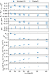 |
Fig. 1. Configuration space RSD results from fits to the average clustering of 25 LRG cubic-box N-body simulations as a function of the minimum separation scale, rmin. Best-fit values of q∥, q⊥, df, and dm are compared to their expected values in the top panels. The mid panel shows the reduced chi-squared rχ2, and the bottom three panels display estimated uncertainties σq∥, σq⊥, σdf, and σdm. Filled markers represent the baseline fit while empty markers indicate fits that include the additional ShapeFit parameter m. |
The mid panel of Fig. 1 displays the reduced chi-squared, rχ2 ≡ χ2/(Nbins − Npar). As expected, the rχ2 values increase for decreasing rmin. Scales below 30 h−1 Mpc exhibit rχ2 > 3, indicating a poor fit and suggesting that the model breaks down on such scales. As rmin increases to approximately 40 h−1 Mpc, the rχ2 stabilizes around 1, reflecting improved agreement between the model and the data.
The last four rows of Fig. 1 display the uncertainties σq∥, σq⊥, σdf and σdm of the parameters of interest. Uncertainties naturally become larger with increasing rmin. Consistent with past works, all values of σq∥ are approximately twice as large as those for σq⊥.
Our baseline choice for CS analysis aims at maximizing the information extracted from the correlation function while obtaining unbiased results on cosmological parameters and a good quality of fit. Based on the results just discussed, we set our baseline choice for our CS analysis to rmin = 30 h−1 Mpc. It is worth noting that we also tested the inclusion of stochastic terms, similar to those used in Fourier space, within the configuration space analysis. This addition helps regularize small scales beyond 30 h−1 Mpc, reducing the reduced χ2 for rmin = 25 h−1 Mpc to 1.6.
Figure 2 presents the similar analysis as Fig. 1 but for Fourier space (FS) and both joint space analyses (JS and JSsep). Here, we are interested in the impact of varying the maximum wavenumber kmax.
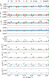 |
Fig. 2. Same as Fig. 1 but for Fourier space (FS, red circles) and the joint space analyses (JS and JSsep, gray circles and green squares, respectively). For reference, CS results for rmin = 30 h−1 Mpc are shown in blue. |
Focusing first on FS results in Fig. 2 (red points), both q∥ and q⊥ show deviations below 1 percent and df below 3 percent for all kmax. The reduced chi-squared rχ2 remains stable, slightly below 1.4, comparable to CS results at rmin = 30 h−1 Mpc. The uncertainties on σq⊥ and σf are notably larger than in CS, expect for kmax ≥ 0.22 h Mpc−1 where they are comparable. Note that FS includes three additional parameters (shot-noise terms), which reduce its constraining power relative to the CS analysis. In the following, we restrict our analysis to kmax = 0.20 h Mpc−1, a choice that is justified later when discussing the joint results. Figure 2 also presents the joint-space results, which is discussed later.
Focusing now in the JS analysis in Fig. 2 (gray circles), we observe small shifts on the best-fit values of all three parameters compared to FS or CS, though not significant. Regarding estimated uncertainties, JS yields uncertainties comparable to, or smaller than, those in CS, indicating some small gain in the combination with FS. However, rχ2 values are significantly higher for JS, with values above 2.5 and increasing with kmax, indicating a poor fit at this statistical precision level. As we discuss next, the quality of the JS fit is degraded due to tensions in some of the nuisance parameters between CS and FS. For this reason, we perform a modified joint analysis where parameters b2, bs, α0, α2, and α4 are allowed to vary independently in the power spectrum and correlation function models. This alternative approach is referred to as JSsep. Figure 2 presents the JSsep results (gray squares), as a function of kmax. The overall performance of the fit is comparable to the standard JS analysis, though we note significant a reduction in rχ2 to ∼1.5, comparable to CS and FS fits. For kmax > 0.20 h Mpc−1, the JSsep results for f and dm exhibit some discrepancies. Given those results, we set the baseline choice of kmax = 0.20 h Mpc−1 for FS, JS and JSsep.
Figure 3 presents the best-fit models with our baseline choice of separations (30 < r < 150 h−1 Mpc and 0.02 < k < 0.20 h Mpc−1) of our two-point multipoles (ℓ = 0, 2, 4), along with their respective residuals in the lower panels. The differences between the models and the measurements remain within a 2σ deviation, except for the hexadecapole in CS. We remind that neighboring separations in CS measurements are strongly correlated (Fig. A.1) so these deviations are not significant.
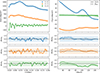 |
Fig. 3. Fourier space (FS) power spectrum multipoles (left panel) and correlation function (CS) multipoles (right panel) with their best-fit models. We consider the monopole (blue), quadrupole (orange), and hexadecapole (green) in both spaces. The three bottom panels show the normalized residuals and the shaded areas correspond to 2σ. The best-fit model of FS and CS are shown in solid lines while the joint-space JSsep model is represented with a dashed line. |
Figure 4 shows the 68 and 95 percent contours of all parameter posteriors for FS, CS and JS. Posteriors in both FS and CS are in good agreement for all parameters, though CS constraints tend to be tighter (e.g., b2, bs, α0). For JS, contours for q∥ and q⊥ exhibit slightly larger biases compared to individual analyses, although they remain within 2σ. Surprisingly, the JS constraints on b1, b2, α2 and α4 are inconsistent with the FS and CS results. This might be due to the breaking of degeneracies in a multi-dimensional parameter space. An important caveat is that our JS fits use a sample covariance from 1000 mocks, though the data vector is larger. This covariance is thus noisier for JS compared to FS or CS (see Table 2), which might shift contours. Given the large cross-covariance between FS and CS (as illustrated in Fig. A.1), posteriors might be more sensitive to sample noise. To test this hypothesis, we computed JS posterior while neglecting the cross-covariance between FS and CS multipoles. These posteriors are shown in dashed lines in Fig. 4, now in good agreement with the FS-CS contours, as expected when combining two independent likelihoods. We also tested fits on the average of 1000 EZMOCKS (both DESI and eBOSS versions), using covariance matrices derived from the same set of mocks. This guarantees a correct covariance treatment in the fit, as it is directly derived from the same mocks used for the average. For both EZMOCKS sets, no significant bias is observed between CS, FS, and JS analyses. All three posteriors are fully consistent, in contrast to the bias seen in Fig. 4 for JS when using cubic box mocks. We then compared the results of Fig. 4 with the best-fit values obtained using IMINUIT. For all analyses, the IMINUIT best-fit points lie at the center of the contours, except for bs and b2 which can be due to the presence of local maximum in the likelihood. This supports the bias observed for b1, α2, and α4. We also test the impact of the finite number of mocks used to compute the covariance by using 500 instead of 1000 mocks. No significant difference was seen, which discards the impact of the limited number of mocks. These tests could indicate that the cross terms in a covariance matrix derived from 1000 EZMOCKS are not accurate enough when fitting N-body simulations.
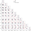 |
Fig. 4. Likelihood posterior (1σ − 2σ) for FS (red), CS (blue), and JS (gray) obtained from fits to the average of the 25 LRG CubicBox mocks. JS contours without the cross covariance (labelled “w/o crosscov”) are displayed in dashed gray. The dotted black lines represent the expected values. Results are shown for kmax = 0.20 h Mpc−1 and rmin = 30 h−1 Mpc. |
Figure 5 presents posteriors for FS, CS (same as in Fig. 4) as well as those from the JSsep analysis and the Gaussian approximation method (GA; see Sect. 3.2). All four contours are consistent with each other within 1σ. The GA contours tend to fall between the FS and CS contours, while the JSsep do not show significant bias in the four parameters of interest to the separate analyses.
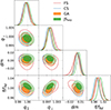 |
Fig. 5. Contours of 68 and 95 percent of the posterior distributions for FS (red), CS (blue), JSsep (green), and GA (orange) derived from fits to the average clustering of 25 LRG cubic-box mocks from N-body simulations. |
Additionally, JSsep does not show any notable improvement over GA when tested on the average of the 25 mocks, as both yield similar results.
These tests validate our baseline choices for the analyses and we turn to the study of a large set of mock catalogs.
5.2. Fits to 1000 eBOSS LRG EZmocks
We evaluated the statistical properties of our best-fit values and their uncertainties with fits to 1000 realizations of eBOSS LRG EZMOCKS, which reproduce realistic angular and redshift distributions (see Sect. 2). These mocks allow us to assess how the results on individual realizations compare to their corresponding distributions, and check that our uncertainties are correctly estimated. We computed two-point multipoles for all realizations and derived their corresponding sample covariance matrix (Eq. (2)).
We used the frequentist approach to fit individual mocks (see Sect. 3) as it is faster than the Bayesian approach.
Figure 6 compares the distributions of best-fit parameters in FS (y-axis) and CS (x-axis) for the 1000 individual eBOSS EZMOCKS. The top row displays the best-fit values for q∥, q⊥, and f, while the bottom row shows their estimated errors σq∥, σq⊥, and σf. The density of points is represented by grayscale shading, and the diagonal dashed line is the identity line. The distribution of the best-fit values is well correlated and mostly scattered around the identity line, except for q∥, which tends to have slightly higher values in FS than in CS.
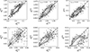 |
Fig. 6. Comparison of the RSD measurements in FS (y-axis) and CS (x-axis) for the individual 1000 EZMOCKS of the eBOSS LRG sample. The top row displays the best-fit values for q∥, q⊥, and f, while the bottom row shows their estimated errors σq∥, σq⊥, and σf. The density of points is represented by grayscale shading, with dashed lines indicating the line of perfect correlation where the compared parameters are equal. We display the Pearson correlation coefficients between CS and FS. The plus symbol represents the results from the real eBOSS data, as listed in Table 6. |
The discrepancy seen for q∥ in FS may be due to non-Gaussian effects in the posteriors of parameters, which could be caused by the volume difference between the large effective volume of the covariance and the smaller volume of individual mocks. To mitigate this effect, we combine the 1000 EZMOCKS in groups of 5, making a total of 200 independent EZMOCKS with a volume 5 times larger. The discrepancy in FS is still present, which discards this hypothesis. We simply think that this bias is due to the approximate nature of EZMOCKS and that it is not guaranteed that the recovered cosmological parameters are aligned with the expected value, unlike ABACUS cubic boxes. We also performed a BAO fit on the average of the 1000 EZMOCKS, and both CS and FS recovered the expected value, while the full-shape fit on this average still shows the bias. This may indicate that when the fit is limited to higher scales as in the BAO case, the results are not biased, which confirms that the issue is related to the approximations in EZMOCKS. The uncertainties show good agreement overall for q∥ and q⊥, but for f, CS uncertainties are larger than FS on average.
Statistics on the fit of the 1000 eBOSS LRG EZmocks realizations.
Best-fit parameters from the eBOSS DR16 LRG sample using different methods.
We computed consensus results using the Gaussian approximation method (GA) for each mock realization. First, we construct the 6 × 6 parameter covariance matrix from the 1000 eBOSS EZMOCKS best-fit values of q∥, q⊥ and f. Figure A.2 displays the resulting correlation matrix, where we can notice in particular that the correlations for q∥, q⊥ and fσ8 are 61, 51 and 81 percent, respectively, between CS and FS. Second, we computed consensus parameters and their corresponding covariances for each mock realization, adjusting each time the off-diagonal blocks of the parameter covariance (see Sect. 3.2).
Figure 7 shows the distributions of q∥, q⊥, f, and their associated errors σq∥, σq⊥, σf, as estimated with the GA method, compared to the same quantities obtained from CS and FS. The distribution of the best-fit values is well correlated and generally scattered around the identity line, except for q∥, where the scatter between GA and CS is slightly smaller than that between GA and FS. This suggests a higher weight of CS in the GA analysis compared to FS. Additionally, the errors estimated by GA are systematically smaller than those obtained in either CS or FS analyses. It is worth noting that the distribution of σf splits into two distinct clouds, as shown in Fig. 6.
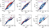 |
Fig. 7. Comparison of the RSD measurements in FS (red) and CS (blue) with GA on the individual 1000 eBOSS EZmock. FS and CS results are shown on the y-axis, while GA results are on the x-axis. The top row displays the best-fit values for q∥, q⊥, and fσ8, while the bottom row shows their estimated errors σq∥, σq⊥, and σfσ8. The density of points is represented by the color-scale shading, and the dashed lines indicate the line of perfect correlation where the compared parameters are equal. We display the Pearson correlation coefficients between GA and FS, as well as GA and CS. The plus symbols represent the best-fit results from the real eBOSS data as listed in Table 6. |
Figure 8 is analogous to Fig. 7 but for the results from the JSsep method. Similar to the GA results, the best-fit values are well-correlated and closely cluster around the identity line. However, the scatter is noticeably more pronounced in JSsep compared to GA.
While JSsep uncertainties are consistently smaller than or similar to those observed in CS and FS, they exhibit greater scatter relative to the GA results shown in Fig. 7. This scatter is due to the different nature of the fit, which now incorporates the cross-covariance between FS and CS at the level of the two-point functions. These noisy terms (due to a limited number of mocks) are propagated to the final infered parameters. The similar or smaller uncertainties show that there is gain in combining FS and CS results at the two-point level, even though they are highly correlated.
Table 5 summarizes the statistical properties of (q∥, q⊥, f) for CS, FS, GA, and JSsep. For each parameter p, we show the average bias with respect to its expected value, Δp = ⟨pi − pexp⟩, the standard deviation of best-fit values σp, the mean estimated error ⟨σpi⟩, the mean of the pull  , and its standard deviation. If the parameter uncertainties are correctly estimated and follow a Gaussian distribution, we expect σp = ⟨σpi⟩, ⟨Zpi⟩ = 0 and σZpi = 1. The table also includes the mean value of the reduced chi-square, rχmin2. From this table, we observe:
-
the number of valid realizations, Ngood, is nearly maximal for all analyses, indicating that most fits have successfully converged. The discarded cases in FS and GA are due to the removal of outliers beyond the 5σ threshold. For each method, the average minimum reduced chi-square ⟨rχmin2⟩ is close to 1, suggesting that the majority of the mocks are well-modeled, with JSsep exhibiting the closest value from 1.
-
the mean estimated error, ⟨σpi⟩, is generally consistent with the standard deviation of the best-fit values, σp, across all parameters and analyses, indicating no significant issues with the uncertainty estimations. Notably, the mean estimated errors for JSsep are smaller than those for CS, FS, and GA (except for q⊥) which means that there is small gain in performing the joint analysis.
-
the standard deviations of the best-fit values, σp, are consistently smaller in GA compared to JSsep for all three parameters. It is important to note that these standard deviations are scaled by the correction factor
 (Sect. 3.1) and these corrections are different between FS, CS and JS.
 -
the average bias for q∥ is larger in JSsep and FS (more than 3 percent) when compared to GA and CS. The bias in JSsep might be pulled by the large bias seen in FS. The GA results lie between FS and CS as expected, for all parameters. For the growth rate f, JSsep has the smallest bias among all methods.
-
the mean of the pull ⟨Zxi⟩ is consistent with zero for all methods. For f, the smallest value of the mean pull is achieved by JSsep. The standard deviations of the q⊥ and q∥ pulls are slightly larger than 1 in all cases, suggesting that errors are slightly underestimated, with the most significant underestimation for q⊥ in JSsep, of about 30 percent. For f, the standard deviation of JSsep is slightly smaller than 1, indicating a slight overestimation of the error. However, JSsep provides results closest to 1 compared to the other methods.
-
The high value of σZq⊥ observed in JSsep may be due to the limited number of mocks used for the covariance. We recomputed the same statistics presented in Table 5 using a covariance matrix derived from twice fewer mocks, i.e., 500 mocks. The standard deviation of the pull for the three parameters in JSsep increased to ∼4, which may indicate the necessity of using a larger number of mocks for the covariance when performing JS analyses to obtain more reliable uncertainty estimates.
6. Application to the BOSS+eBOSS LRG sample
In this section we apply our methodology to the BOSS+eBOSS LRG sample presented in Sect. 2.1. We present results for Fourier space (FS), configuration space (CS), and our two consensus methods, the Gaussian approximation (GA) and joint space (JSsep).
Figure 9 displays the best-fit models for the power spectrum and correlation function multipoles for the separate analyses (FS and CS, shown as solid lines) and the joint analysis (JSsep, shown as dashed lines). The residuals are shown in the bottom panels, highlighting good agreement between JSsep and CS/FS, which we attribute to differences in the inferred bias and counterterms.
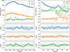 |
Fig. 9. Best-fit models for the monopole, quadrupole, and hexadecapole of BOSS+eBOSS LRG sample in Fourier-space (left panel, solid line) and configuration space (right panel, solid line). The bottom three subpanels display the normalized residuals, with shaded areas indicating a 2σ range. The best-fit model for joint space fit, JSsep, is shown as a dashed line. |
Figure 10 shows the contours of the posterior distribution (1σ and 2σ) for the FS, CS, GA, and JSsep analyses, all of which are in good agreement. The posteriors are consistent with one another (within 1σ), displaying comparable widths except for f in CS, which shows a higher value with a significantly larger width, though consistent with the behavior seen in eBOSS mocks (Fig. 6), and the posterior of m for GA which is completly biased by more than 2σ) The JSsep posterior is consistent with the other posteriors and comparable to GA, though we can see how these contours are not exactly Gaussian, which is one of the advantages of the method.
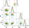 |
Fig. 10. Likelihood posterior for FS (red), CS (blue), JSsep (green), and GA (orange) derived from fits on the eBOSS LRG data. |
Figure 10 shows the contours of the posterior distribution (1σ and 2σ) for the FS, CS, GA, and JSsep analyses, all of which are in good agreement. The posteriors are consistent with one another (within 1σ), displaying comparable widths except for f in CS, which shows a higher value with a significantly larger uncertainty. This behavior is consistent with what we observe in the eBOSS mocks (Fig. 6). The posterior of m in GA, however, is significantly biased, deviating by more than 2σ, illustrating the limitations of the GA method when the posteriors are non-Gaussian, as is the case for this parameter in CS. The JSsep posterior remains consistent with the other estimates and closely tracks GA, except for m, although its contours exhibit non-Gaussian features–highlighting one of the key strengths of the joint-space approach.
Table 6 summarizes the results of the four different analyses. The reduced χ2 values are 1.82, 1.10, and 1.34 for FS, CS, and JSsep, respectively. The high χ2 value of FS represents a deviation greater than 3σ compared to the distribution of χ2 from EZMOCK eBOSS. The best-fit values for the parameters q∥, q⊥, and fσ8 are all consistent within their respective 1σ errors. For q∥ and q⊥, JSsep provides the smallest uncertainties while yielding the highest and lowest best-fit values, respectively, compared to the other methods. Additionally, JSsep yields a slightly smaller value for fσ8, similar to the one from CS. Still in Table 6, we compare our main JSsep results with the official RSD results from Gil-Marín et al. (2020), FS eBOSS), Bautista et al. (2021), CS eBOSS), and the consensus between the two (GA eBOSS). The main difference between our analysis and official ones lies in the modeling approach. Previous analyses employed the TNS model (Taruya et al. 2010), which is based on an Eulerian description and incorporates a damping term for fingers-of-God rather than counterterms. The scale ranges are the same for both CS analyses while for FS, we increased from kmax = 0.15 to 0.20 h Mpc−1.
Our final result on this dataset using our JSsep method yields
 (22)
(22)
Our results are compatible with all three analyses but show a slightly lower value for q∥, a higher value for q⊥, and for fσ8. These discrepancies can largely be attributed to differences in the clustering models, the scale ranges, the inclusion of cross-covariance terms in the JS analysis, and the inclusion of systematic errors (in the case of the official ones). Uncertainties on q∥ are notably larger than in the official eBOSS results, likely due to the inclusion of additional counterterms and shot noise terms in our model, which introduce μ2 and μ4 dependencies (see Eq. (13)).
7. Conclusion
This work presents a new RSD analysis of the DR16 LRG sample (BOSS+eBOSS), where we extract cosmological parameters simultaneously from the configuration-space and Fourier-space two-point multipoles. We compared the joint-space (JS) approach to obtain consensus results with the commonly used Gaussian approximation (GA), which combines CS and FS results at the parameter level, assuming Gaussian posteriors.
To validate our methodology, we first applied it to the average of 25 N-body LRG cubic-box mocks from the AbacusSummit simulation. We assessed parameter consistency between CS and FS and compared JS results with each individual space. Unexpected behavior was observed for parameters such as b2, α2, and α4, with 1σ–2σ deviations from CS and FS, possibly due to noisy cross-terms in the covariance matrix. Allowing parameters b2, bs, and the counterterms to vary independently in JS (JSsep) led to unbiased results with a reduced rχ2 = 1.5. However, JS did not show significant improvements over CS, FS, or GA when tested on the mock average. Further tests were conducted on 1000 LRG EZmocks, which reproduce the DR16 LRG sample geometry. We found JS results to be consistently smaller than those of CS and FS but with greater scatter compared to GA.
After validation of our framework, we applied it to real data of the DR16 LRG multipoles. The JS method provided the tightest constraints on q∥, q⊥, and fσ8, remaining consistent with the official 2020 results from Bautista et al. (2021) and Gil-Marín et al. (2020). However, JSsep yielded the highest value for fσ8 = 0.463 ± 0.052, which we attribute to differences in modeling and the inclusion of cross-covariance terms between FS and CS.
We believe our framework is more robust than FS, CS, or GA approaches and should be used in future surveys. Systematic effects in either space are averaged out at the multipole level, providing unbiased constraints on the growth rate and dilation parameters. Future work employing our methods will pay attention to the precision of covariance matrices estimates, as the large noise might affect the final constraints.
Acknowledgments
The project leading to this publication has received funding from Excellence Initiative of Aix-Marseille University – A*MIDEX, a French “Investissements d’Avenir” program (AMX-20-CE-02 – DARKUNI). Thanks to NERSC.
References
- Ahumada, R., Allende Prieto, C., Almeida, A., et al. 2020, ApJS, 249, 3 [NASA ADS] [CrossRef] [Google Scholar]
- Alam, S., Ata, M., Bailey, S., et al. 2017, MNRAS, 470, 2617 [Google Scholar]
- Alam, S., Aubert, M., Avila, S., et al. 2021, Phys. Rev. D, 103, 083533 [NASA ADS] [CrossRef] [Google Scholar]
- Alcock, C., & Paczynski, B. 1979, Nature, 281, 358 [NASA ADS] [CrossRef] [Google Scholar]
- Ballinger, W. E., Peacock, J. A., & Heavens, A. F. 1996, MNRAS, 282, 877 [NASA ADS] [CrossRef] [Google Scholar]
- Baumann, D., Nicolis, A., Senatore, L., & Zaldarriaga, M. 2012, JCAP, 07, 051 [CrossRef] [Google Scholar]
- Bautista, J. E., Paviot, R., Vargas Magaña, M., et al. 2021, MNRAS, 500, 736 [Google Scholar]
- Bernardeau, F., Colombi, S., Gaztanaga, E., & Scoccimarro, R. 2002, Phys. Rep., 367, 1 [NASA ADS] [CrossRef] [Google Scholar]
- Beutler, F., & McDonald, P. 2021, JCAP, 11, 031 [Google Scholar]
- Beutler, F., Castorina, E., & Zhang, P. 2019, JCAP, 03, 040 [Google Scholar]
- Blanton, M. R., Bershady, M. A., Abolfathi, B., et al. 2017, AJ, 154, 28 [Google Scholar]
- Brieden, S., Gil-Marín, H., & Verde, L. 2021, JCAP, 12, 054 [Google Scholar]
- Cabass, G., Ivanov, M. M., Lewandowski, M., Mirbabayi, M., & Simonović, M. 2022, arXiv e-prints [arXiv:2203.08232] [Google Scholar]
- Carlson, J., Reid, B., & White, M. 2013, MNRAS, 429, 1674 [NASA ADS] [CrossRef] [Google Scholar]
- Carrasco, J. J. M., Hertzberg, M. P., & Senatore, L. 2012, JHEP, 09, 082 [CrossRef] [Google Scholar]
- Chen, S.-F., Vlah, Z., & White, M. 2020, JCAP, 07, 062 [Google Scholar]
- Chen, S.-F., Vlah, Z., Castorina, E., & White, M. 2021, JCAP, 03, 100 [Google Scholar]
- Chuang, C.-H., Kitaura, F.-S., Prada, F., Zhao, C., & Yepes, G. 2015, MNRAS, 446, 2621 [NASA ADS] [CrossRef] [Google Scholar]
- Dawson, K. S., Schlegel, D. J., Ahn, C. P., et al. 2013, AJ, 145, 10 [Google Scholar]
- Dawson, K. S., Kneib, J.-P., Percival, W. J., et al. 2016, AJ, 2, 44 [Google Scholar]
- de Mattia, A., Ruhlmann-Kleider, V., Raichoor, A., et al. 2020, MNRAS, 501, staa3891 [Google Scholar]
- DESI Collaboration (Aghamousa, A., et al.) 2016a, arXiv e-prints [arXiv:1611.00036] [Google Scholar]
- DESI Collaboration (Aghamousa, A., et al.) 2016b, arXiv e-prints [arXiv:1611.00037] [Google Scholar]
- DESI Collaboration (Abareshi, B., et al.) 2022, AJ, 164, 207 [NASA ADS] [CrossRef] [Google Scholar]
- DESI Collaboration (Adame, A. G., et al.) 2024, AJ, 168, 58 [NASA ADS] [CrossRef] [Google Scholar]
- DESI Collaboration (Adame, A. G., et al.) 2025a, JCAP, 07, 017 [Google Scholar]
- DESI Collaboration (Adame, A. G., et al.) 2025b, JCAP, 01, 124 [Google Scholar]
- DESI Collaboration (Adame, A. G., et al.) 2025c, JCAP, 02, 021 [CrossRef] [Google Scholar]
- DESI Collaboration (Adame, A. G., et al.) 2025d, JCAP, 04, 012 [Google Scholar]
- DESI Collaboration (Adame, A. G., et al.) 2025e, JCAP, 09, 008 [Google Scholar]
- DESI Collaboration (Adame, A. G., et al.) 2025f, JCAP, 07, 028 [Google Scholar]
- Dumerchat, T., & Bautista, J. E. 2022, A&A, A80 [NASA ADS] [CrossRef] [EDP Sciences] [Google Scholar]
- Eisenstein, D. J., Weinberg, D. H., Agol, E., et al. 2011, AJ, 142, 72 [Google Scholar]
- Foreman-Mackey, D., Hogg, D. W., Lang, D., & Goodman, J. 2013, PASP, 125, 306 [Google Scholar]
- Garrison, L. H., Eisenstein, D. J., & Pinto, P. A. 2019, MNRAS, 485, 3370 [CrossRef] [Google Scholar]
- Garrison, L. H., Eisenstein, D. J., Ferrer, D., Maksimova, N. A., & Pinto, P. A. 2021, MNRAS, 508, 575 [NASA ADS] [CrossRef] [Google Scholar]
- Gelman, A., & Rubin, D. B. 1992, Stat. Sci., 4, 457 [Google Scholar]
- Gil-Marín, H., Bautista, J. E., Paviot, R., et al. 2020, MNRAS, 498, 2492 [Google Scholar]
- Grieb, J. N., Sánchez, A. G., Salazar-Albornoz, S., & Vecchia, C. D. 2016, MNRAS, 457, 1577 [NASA ADS] [CrossRef] [Google Scholar]
- Gunn, J. E., Siegmund, W. A., Mannery, E. J., et al. 2006, AJ, 131, 2332 [NASA ADS] [CrossRef] [Google Scholar]
- Hadzhiyska, B., Eisenstein, D., Bose, S., Garrison, L. H., & Maksimova, N. 2022, MNRAS, 509, 501 [Google Scholar]
- Hartlap, J., Simon, P., & Schneider, P. 2007, A&A, 464, 399 [NASA ADS] [CrossRef] [EDP Sciences] [Google Scholar]
- Hou, J., Sánchez, A. G., Ross, A. J., et al. 2021, MNRAS, 500, 1201 [Google Scholar]
- Ivanov, M. M. 2022, arXiv e-prints [arXiv:2212.08488] [Google Scholar]
- Kaiser, N. 1987, MNRAS, 227, 1 [Google Scholar]
- Landy, S. D., & Szalay, A. S. 1993, AJ, 412, 64 [Google Scholar]
- Matsubara, T. 2008a, Phys. Rev. D, 78, 109901 [Google Scholar]
- Matsubara, T. 2008b, Phys. Rev. D, 77, 063530 [NASA ADS] [CrossRef] [Google Scholar]
- Matsubara, T. 2015, Phys. Rev. D, 92, 023534 [Google Scholar]
- Maus, M., Chen, S., White, M., et al. 2024, arXiv e-prints [arXiv:2404.07312] [Google Scholar]
- McDonald, P., & Roy, A. 2009, JCAP, 08, 020 [CrossRef] [Google Scholar]
- Neveux, R., Burtin, E., de Mattia, A., et al. 2020, MNRAS, 499, 210 [NASA ADS] [CrossRef] [Google Scholar]
- Percival, W. J., Ross, A. J., Sánchez, A. G., et al. 2014, MNRAS, 439, 2531 [NASA ADS] [CrossRef] [Google Scholar]
- Rampf, C. 2012, JCAP, 12, 004 [Google Scholar]
- Ross, A. J., Bautista, J., Tojeiro, R., et al. 2020, MNRAS, 498, 2354 [NASA ADS] [CrossRef] [Google Scholar]
- Sánchez, A. G., Grieb, J. N., Salazar-Albornoz, S., et al. 2017, MNRAS, 464, 1493 [CrossRef] [Google Scholar]
- Smee, S. A., Gunn, J. E., Uomoto, A., et al. 2013, AJ, 146, 32 [Google Scholar]
- Tamone, A., Raichoor, A., Zhao, C., et al. 2020, MNRAS, 499, 5527 [Google Scholar]
- Taruya, A., Nishimichi, T., & Saito, S. 2010, Phys. Rev. D, 82, 063522 [NASA ADS] [CrossRef] [Google Scholar]
- Taylor, A. N., & Hamilton, A. J. S. 1996, MNRAS, 282, 767 [NASA ADS] [Google Scholar]
- Vlah, Z., White, M., & Aviles, A. 2015, JCAP, 09, 014 [CrossRef] [Google Scholar]
- Vlah, Z., Castorina, E., & White, M. 2016, JCAP, 12, 007 [Google Scholar]
- White, M. 2014, MNRAS, 439, 3630 [NASA ADS] [CrossRef] [Google Scholar]
- Yamamoto, K., Nakamichi, M., Kamino, A., Bassett, B. A., & Nishioka, H. 2006, PASJ, 58, 93 [Google Scholar]
- Yuan, S., Zhang, H., Ross, A. J., et al. 2023, MNRAS, 530, 947 [Google Scholar]
- Zel’dovich, Y. A. B. 1970, A&A, 5, 84 [Google Scholar]
- Zhao, C., Chuang, C.-H., Bautista, J., et al. 2021, MNRAS, 503, 1149 [CrossRef] [Google Scholar]
A specific value of ξ(r) at separation r is a weighted integral of P(k) over a broad range of k values. Consequently, unless the r and k ranges used in the analyses are infinite, these approaches do not contain the same information.
Appendix A: Covariance matrix
Figure A.1 shows the correlation matrix R, defined as
![Mathematical equation: $$ \begin{aligned} \boldsymbol{R} = \boldsymbol{\sigma }^{-1}\boldsymbol{\hat{C}} [\boldsymbol{\sigma }^{-1}]^T, \end{aligned} $$](/articles/aa/full_html/2026/02/aa56020-25/aa56020-25-eq41.gif) (A.1)
(A.1)
where σ is derived from the square root of the diagonal elements of the covariance matrix  . Beyond the well-known correlations between multipoles in the same space, the structure of the off-diagonal blocks reveals the correlation dynamics between the two distinct spaces. The multipole-multipole correlations between these spaces exhibit similar patterns. This arises due to the Fourier transform, which links a specific physical scale r with multiple spectral modes k. At a given scale r, there are notable correlations (and anti-correlations) with several k modes. This indicates that statistical information from a physical scale is distributed across multiple spectral modes rather than being confined to a single mode. These oscillations seen in the covariance can be derived analytically following Grieb et al. (2016) and shown in Appendix C of Dumerchat & Bautista (2022).
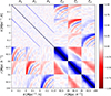 |
Fig. A.1. Normalized covariance matrix of the power spectrum multipoles P0, 2, 4 and the correlation function multipoles ξ0, 2, 4, measured from the 1000 cubic-box EZMOCKS of LRGs. |
Figure A.2 shows the correlation matrix of the parameters q∥, q⊥ and fσ8, obtained from 1000 fits to the eBOSS LRG EZmocks. This matrix is used to obtain the Gaussian approximation consensus results in Sect. 5.
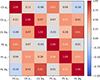 |
Fig. A.2. Correlation coefficients between q⊥, q∥, and fσ8 for CS and FS, derived from fits to the 1000 EZMOCKS of the eBOSS LRG sample. |
Appendix B: Clustering model
We use a Lagrangian perturbation theory (LPT) model to describe the observed clustering in both configuration and Fourier space. This model is based on the Lagrangian formalism developed in Chen et al. (2020, 2021). In this section we provide a brief overview of this formalism.
B.1. Lagrangian perturbation theory
In the Lagrangian picture, cosmological structure formation is modeled by following the trajectories of fluid elements rather than studying the dynamics of density and velocity fields. The variable of interest in LPT is the displacement field Ψ(q, η), which corresponds to the difference between the Lagrangian coordinates q (at some initial time η0) and the Eulerian coordinates x(q) of a fluid element at a given conformal time η:
 (B.1)
(B.1)
where Ψ(q, η0) = 0. Each element of the fluid is labeled by q, and Ψ(q, η) fully describes its evolution. The Eulerian density field ρ(x, η) satisfies the continuity relation:
 (B.2)
(B.2)
where  is the mean density in comoving coordinates.
We can define the Jacobian of the transformation between Eulerian and Lagrangian coordinates as ![Mathematical equation: $ J = \det\left[\frac{\partial \mathbf{x}}{\partial \boldsymbol{q}}\right] $](/articles/aa/full_html/2026/02/aa56020-25/aa56020-25-eq46.gif) :
:
 (B.3)
(B.3)
Using the definition of the density contrast ![Mathematical equation: $ \rho(\mathbf{x}, \eta) = \bar{\rho}(\eta) \left[1 + \delta(\mathbf{x}, \eta)\right] $](/articles/aa/full_html/2026/02/aa56020-25/aa56020-25-eq48.gif) and Eqs. B.2 and B.3, we can relate the density contrast to the displacement field:
and Eqs. B.2 and B.3, we can relate the density contrast to the displacement field:
 (B.4)
(B.4)
This relation is equivalent to the following equation:
![Mathematical equation: $$ \begin{aligned} 1 + \delta (\mathbf x , \eta ) = \int d^3q \, \delta _D\left[\mathbf x - \boldsymbol{q} - \Psi (\boldsymbol{q}, \eta )\right]. \end{aligned} $$](/articles/aa/full_html/2026/02/aa56020-25/aa56020-25-eq50.gif) (B.5)
(B.5)
Fourier transforming Eq. B.5 (in x-space) gives
 (B.6)
(B.6)
The equation of motion for particle trajectories x(η) is
 (B.7)
(B.7)
From which we can infer the evolution equation of Ψ using Eq. B.1:
 (B.8)
(B.8)
where overdots indicate derivatives w.r.t. conformal time η. This equation is solved order by order in a perturbative way such that:
 (B.9)
(B.9)
The first-order solution of LPT Ψ(1) is known as the Zel’dovich approximation (Zel’dovich 1970),
 (B.10)
or equivalently,
 (B.11)
where D+(η) is the linear growth factor and δ0(q) is the initial density contrast. The Zel’dovich approximation uses the linear displacement field to model cosmic structure formation. One can find more details on the Zel’dovich approximation in White (2014). Higher-order solutions are expressed as integrals of higher powers of the linear density field (Matsubara 2015).
Unlike in SPT, there is no simple recursive solution for order-by-order expression in LPT due to the fact that the displacement fields in LPT are not irrotational in general (Rampf 2012; Matsubara 2015).
B.2. Effective field theory of large-scale structures
In this work we use the Effective Field Theory of large-scales structures (EFTofLSS). The main insight is that the LSS has various hierarchical distance scales. In the large scale limit, only the large-scale degrees of freedom are required, while the effects of unknown short-scale physics can be systematically captured by effective operators. This decoupling framework forms the core of the EFTofLSS (Baumann et al. 2012; Carrasco et al. 2012; Cabass et al. 2022; Ivanov 2022). The Lagrangian form of EFT involves smoothing Eq. B.8 and incorporating small-scale physics through a series of counterterms.
To achieve this, we used a filter WR(q, q′), which separates the system into long-wavelength (L) and short-wavelength (S) modes:
 (B.12)
 (B.13)
We can write the displacement as
 (B.14)
where the first three terms come from the perturbative treatment of the long-wavelength evolution and the last two terms parameterize the impact of the short-wavelength modes on the evolution where α1 is a counterterm coefficient and S is equivalent to a stochastic term
B.3. Redshift-space distortions
Before writing the power spectrum we need to include bias scheme. The density of biased tracers can be modeled, assuming Lagrangian bias, by multiplying the δD in the above equation by the bias functional ![Mathematical equation: $ F\left[\delta_0(\boldsymbol q), \boldsymbol\nabla^2 \delta_0(\boldsymbol q), ...\right] $](/articles/aa/full_html/2026/02/aa56020-25/aa56020-25-eq60.gif) depending on linear density and its derivative. The bias functionnal is described by Eq. 4.4 in Chen et al. (2020), more details about the modeling of biased tracers in the Lagrangian picture can be found in Matsubara (2008a), McDonald & Roy (2009) and Vlah et al. (2016). Equation B.6 simply becomes for biased tracers:
depending on linear density and its derivative. The bias functionnal is described by Eq. 4.4 in Chen et al. (2020), more details about the modeling of biased tracers in the Lagrangian picture can be found in Matsubara (2008a), McDonald & Roy (2009) and Vlah et al. (2016). Equation B.6 simply becomes for biased tracers:
 (B.15)
The power spectrum P(k) can be expressed by the displacement field using Eq.(B.15):
 (B.16)
where we have defined the pairwise Lagrangian displacement  . The cumulant theorem allows us to write the expectation value of the exponential in terms of the exponential of expectation values. The cumulant theorem is well defined in Bernardeau et al. (2002), Matsubara (2008a,b) and can be expressed as
![Mathematical equation: $$ \begin{aligned} \left < e^{-iX}\right> = \exp \left[\sum _{N = 1}^\infty \frac{(-i)^N}{N!} \left < X^N\right>_c\right] \end{aligned} $$](/articles/aa/full_html/2026/02/aa56020-25/aa56020-25-eq64.gif) (B.17)
(B.17)
where 〈XN〉c is the cumulant of a random variable X. The bracketed average in Eq. (B.16) can be expressed as
 (B.18)
where  and
and  are the cumulants of the pairwise displacements. More details of those terms can be found on Vlah et al. (2015), Chen et al. (2021).
The power spectrum in Eq. B.16 is valid at all times, not only on the linear regime. From Taylor & Hamilton (1996) we can express the power spectrum in the Zel’dovich approximation. In the Zel’dovich approximation, the displacement field is assumed to be Gaussian at all times. The expectation value of the exponential in Eq. B.16
![Mathematical equation: $$ \begin{aligned} \left< e^{i\boldsymbol{k} \cdot \boldsymbol{\Delta }}\right> = \exp (-k_ik_j\left[ \Psi _{ij}(0) - \Psi _{ij}(\boldsymbol{q})\right]) ,\end{aligned} $$](/articles/aa/full_html/2026/02/aa56020-25/aa56020-25-eq68.gif) (B.19)
(B.19)
with q = q1 − q2 and
 (B.20)
Using the Zel’dovich solution Eq.B.11 we can relate the Ψij(q) to the linear power spectrum (Taylor & Hamilton 1996):
 (B.21)
This results to the Zel’dovich power spectrum:
![Mathematical equation: $$ \begin{aligned} P(\boldsymbol{k}) = \int d^3\boldsymbol{q}\, e^{i\boldsymbol{k} \cdot \boldsymbol{q}}\times \left[e^{\left(-k_ik_j\left[ \Psi _{ij}(\boldsymbol{0}) - \Psi _{ij}(\boldsymbol{q})\right] \right)} - 1\right] \end{aligned} $$](/articles/aa/full_html/2026/02/aa56020-25/aa56020-25-eq71.gif) (B.22)
(B.22)
This equation describes the nonlinear transformation of the initial power spectrum into the evolved power spectrum.
Finally, in the Lagrangian formalism, the RSD can be accounted by boosting displacements along the line-of-sight (LOS) direction  by the velocities of galaxies:
 (B.23)
Where the superscript s is referring to vectors boosted into redshift space and v is the peculiar velocity of galaxy.
The final expression of the theoretical model for the redshift-space galaxy power spectrum, accounting for bias in LPT and EFTofLSS is giving by Eq. 13.
All Tables
Priors on the cosmological and non-cosmological parameters used in our analysis.
All Figures
|
Fig. 1. Configuration space RSD results from fits to the average clustering of 25 LRG cubic-box N-body simulations as a function of the minimum separation scale, rmin. Best-fit values of q∥, q⊥, df, and dm are compared to their expected values in the top panels. The mid panel shows the reduced chi-squared rχ2, and the bottom three panels display estimated uncertainties σq∥, σq⊥, σdf, and σdm. Filled markers represent the baseline fit while empty markers indicate fits that include the additional ShapeFit parameter m. |
| In the text | |
|
Fig. 2. Same as Fig. 1 but for Fourier space (FS, red circles) and the joint space analyses (JS and JSsep, gray circles and green squares, respectively). For reference, CS results for rmin = 30 h−1 Mpc are shown in blue. |
| In the text | |
|
Fig. 3. Fourier space (FS) power spectrum multipoles (left panel) and correlation function (CS) multipoles (right panel) with their best-fit models. We consider the monopole (blue), quadrupole (orange), and hexadecapole (green) in both spaces. The three bottom panels show the normalized residuals and the shaded areas correspond to 2σ. The best-fit model of FS and CS are shown in solid lines while the joint-space JSsep model is represented with a dashed line. |
| In the text | |
|
Fig. 4. Likelihood posterior (1σ − 2σ) for FS (red), CS (blue), and JS (gray) obtained from fits to the average of the 25 LRG CubicBox mocks. JS contours without the cross covariance (labelled “w/o crosscov”) are displayed in dashed gray. The dotted black lines represent the expected values. Results are shown for kmax = 0.20 h Mpc−1 and rmin = 30 h−1 Mpc. |
| In the text | |
|
Fig. 5. Contours of 68 and 95 percent of the posterior distributions for FS (red), CS (blue), JSsep (green), and GA (orange) derived from fits to the average clustering of 25 LRG cubic-box mocks from N-body simulations. |
| In the text | |
|
Fig. 6. Comparison of the RSD measurements in FS (y-axis) and CS (x-axis) for the individual 1000 EZMOCKS of the eBOSS LRG sample. The top row displays the best-fit values for q∥, q⊥, and f, while the bottom row shows their estimated errors σq∥, σq⊥, and σf. The density of points is represented by grayscale shading, with dashed lines indicating the line of perfect correlation where the compared parameters are equal. We display the Pearson correlation coefficients between CS and FS. The plus symbol represents the results from the real eBOSS data, as listed in Table 6. |
| In the text | |
|
Fig. 7. Comparison of the RSD measurements in FS (red) and CS (blue) with GA on the individual 1000 eBOSS EZmock. FS and CS results are shown on the y-axis, while GA results are on the x-axis. The top row displays the best-fit values for q∥, q⊥, and fσ8, while the bottom row shows their estimated errors σq∥, σq⊥, and σfσ8. The density of points is represented by the color-scale shading, and the dashed lines indicate the line of perfect correlation where the compared parameters are equal. We display the Pearson correlation coefficients between GA and FS, as well as GA and CS. The plus symbols represent the best-fit results from the real eBOSS data as listed in Table 6. |
| In the text | |
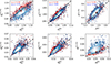 |
Fig. 8. Same as Fig. 7 but for the JSsep method. |
| In the text | |
|
Fig. 9. Best-fit models for the monopole, quadrupole, and hexadecapole of BOSS+eBOSS LRG sample in Fourier-space (left panel, solid line) and configuration space (right panel, solid line). The bottom three subpanels display the normalized residuals, with shaded areas indicating a 2σ range. The best-fit model for joint space fit, JSsep, is shown as a dashed line. |
| In the text | |
|
Fig. 10. Likelihood posterior for FS (red), CS (blue), JSsep (green), and GA (orange) derived from fits on the eBOSS LRG data. |
| In the text | |
|
Fig. A.1. Normalized covariance matrix of the power spectrum multipoles P0, 2, 4 and the correlation function multipoles ξ0, 2, 4, measured from the 1000 cubic-box EZMOCKS of LRGs. |
| In the text | |
|
Fig. A.2. Correlation coefficients between q⊥, q∥, and fσ8 for CS and FS, derived from fits to the 1000 EZMOCKS of the eBOSS LRG sample. |
| In the text | |
Current usage metrics show cumulative count of Article Views (full-text article views including HTML views, PDF and ePub downloads, according to the available data) and Abstracts Views on Vision4Press platform.
Data correspond to usage on the plateform after 2015. The current usage metrics is available 48-96 hours after online publication and is updated daily on week days.
Initial download of the metrics may take a while.