| Issue |
A&A
Volume 706, February 2026
|
|
|---|---|---|
| Article Number | A156 | |
| Number of page(s) | 8 | |
| Section | Planets, planetary systems, and small bodies | |
| DOI | https://doi.org/10.1051/0004-6361/202556674 | |
| Published online | 10 February 2026 | |
Influence of the Martian crustal magnetic fields on oxygen ion escape at Mars
1
Department of Earth and Space Sciences, Southern University of Science and Technology,
Shenzhen,
PR
China
2
Finnish Meteorological Institute,
Helsinki,
Finland
3
Department of Electronics and Nanoengineering, School of Electrical Engineering, Aalto University,
Espoo,
Finland
4
School of Science, Harbin Institute of Technology (Shenzhen),
Shenzhen,
PR
China
5
Swedish Institute of Space Physics,
Uppsala,
Sweden
★ Corresponding author: This email address is being protected from spambots. You need JavaScript enabled to view it.
Received:
31
July
2025
Accepted:
2
January
2026
Abstract
Context. The escape of oxygen ions from Mars has played a crucial role in the planet’s long-term atmospheric evolution and habitability. The crustal magnetic fields influence ion escape, but the exact role remains debated. Previous studies have presented contrasting conclusions, suggesting that the crustal fields may either suppress or enhance oxygen ion escape. To date, the extent and mechanisms of this influence remain insufficiently understood.
Aims. This study aims to investigate the influence of the Martian crustal magnetic fields on the oxygen ion escape at Mars.
Methods. Several groups of 3D global hybrid simulations of Mars-solar wind interaction were performed, with the escaping oxygen ion trajectories traced. The results from the simulations with or without the crustal fields and under different interplanetary magnetic field conditions were then compared.
Results. The simulation results show that the presence of crustal fields enhances the ionospheric oxygen ion escape, while the exospheric oxygen ion escape rate remains largely unaffected. The crustal magnetic fields alter the local electric and magnetic environments and, subsequently, modify the local oxygen ion density and flow direction in the ionosphere. First, the steep magnetic inclination and large magnetic strength in crustal field regions increase the density of low-altitude ionospheric oxygen ions and facilitate their outward transport, thereby promoting ion escape. Second, the crustal fields modify the local electric field structure, which also affects ion acceleration and escape. When strong crustal fields are located on the dayside, their obstruction of the upstream plasma flow weakens the dayside radial electric field at low altitudes in the southern hemisphere. The weakened electric field tends to assist or reduce ion escape, depending on whether it points toward or away from Mars, respectively. In any case, the influence of the magnetic field topology change (the steep magnetic inclination and large magnetic strength) in crustal field regions dominates the effect of weakened electric field, resulting in a higher escape rate than that without the crustal fields. Additionally, when strong crustal fields are on the nightside, the dayside moderate crustal fields still enhance the local density and outward transport of ionospheric oxygen ions, while their impact on the local electric field remains limited. The net effect is enhanced ion escape over the +E hemisphere where the solar wind motional electric field points away from Mars.
Key words: methods: numerical / planet-star interactions / planets and satellites: individual: Mars
© The Authors 2026
 Open Access article, published by EDP Sciences, under the terms of the Creative Commons Attribution License (https://creativecommons.org/licenses/by/4.0), which permits unrestricted use, distribution, and reproduction in any medium, provided the original work is properly cited.
This article is published in open access under the Subscribe to Open model. This email address is being protected from spambots. You need JavaScript enabled to view it. to support open access publication.
1 Introduction
Atmospheric escape plays a critical role in shaping planetary climate and habitability throughout the Solar System’s history. In particular, the escape of heavy ions such as oxygen ions (O+, ![Mathematical equation: $\[\mathrm{O}_{2}^{+}\]$](/articles/aa/full_html/2026/02/aa56674-25/aa56674-25-eq1.png) ) under solar wind interaction is considered a key mechanism responsible for atmospheric loss and planetary evolution (Jakosky et al. 2018). Earth possesses a strong global dipole magnetic field, while Mars lacks a global intrinsic magnetic field, resulting in fundamental differences in their atmospheric escape environments. Earth’s strong dipole field effectively shields its atmosphere from solar wind erosion, whereas Mars experiences direct solar wind interaction with its upper atmosphere, leading to substantial ion loss.
) under solar wind interaction is considered a key mechanism responsible for atmospheric loss and planetary evolution (Jakosky et al. 2018). Earth possesses a strong global dipole magnetic field, while Mars lacks a global intrinsic magnetic field, resulting in fundamental differences in their atmospheric escape environments. Earth’s strong dipole field effectively shields its atmosphere from solar wind erosion, whereas Mars experiences direct solar wind interaction with its upper atmosphere, leading to substantial ion loss.
Although the Martian dynamo ceased approximately four billion years ago, localized crustal magnetic fields remain embedded in the surface rocks, primarily distributed in the southern hemisphere (Acuña et al. 1999). These crustal fields complicate Mars-solar wind interactions by altering the structure of the induced magnetosphere. Previous studies have shown that the crustal fields regulate the location of the bow shock, shape the magnetosphere, trigger magnetic reconnection and auroral emissions, and affect atmospheric escape processes (Dong et al. 2015; Dubinin et al. 2023a; Garnier et al. 2022; Hara et al. 2022; Harada et al. 2015; Wang et al. 2022; DiBraccio et al. 2022; Zhou et al. 2024).
The role of crustal magnetic fields in modulating the Martian oxygen ion escape has been under active investigation, with studies presenting varying conclusions (Nilsson et al. 2011; Fang et al. 2015, 2017; Romanelli et al. 2018; Weber et al. 2021). While strong global magnetic fields are generally believed to inhibit atmospheric loss, localized or weak crustal fields can either suppress or enhance ion escape depending on their spatial configuration (Wei et al. 2014). Dubinin et al. (2023b) proposed that the Martian crustal fields may function analogously to a weak planetary dipole. Kallio & Barabash (2012) demonstrated through hybrid simulations that a weak dipole intrinsic magnetic field can enhance oxygen ion escape, with the escape rate reaching a maximum when the dipole field strength is 10 nT at the magnetic equator on the Martian surface. This enhancement effect of a weak dipole field on the heavy ion escape is later confirmed by the magnetohydrodynamic (MHD) simulations of Sakata et al. (2022). On the other hand, global hybrid simulations suggest that increasing the dipole field further inhibits heavy ion escape (Egan et al. 2019). The Mars Atmosphere and Volatile Evolution (MAVEN) observations also indicate that the crustal fields may partially suppress ion escape (Fan et al. 2019), a result further supported by the MHD modeling by Li et al. (2020).
The overall effect of crustal fields on the Martian oxygen ion escape rate is nontrivial. The observational study by Ramstad et al. (2016) and the MHD simulation results in Ma & Nagy (2007) showed that although the crustal fields shield portions of the ionosphere from direct solar wind impact, they simultaneously cause ionospheric expansion, which may offset the shielding effect. Dubinin et al. (2020) analyzed MAVEN observations and showed that heavy ion escape rates vary with the solar zenith angle due to Mars’ rotation, highlighting the role of local crustal field structures in introducing significant spatial variability of ion escape. Li et al. (2023) further reported that strong dayside crustal fields substantially affect the tailward transport of oxygen ions, and Wang et al. (2024) identified conditions under which these fields enhance the oxygen ion escape rate.
Structural alterations in the magnetosphere associated with the crustal fields further affect ion escape processes. Zhang et al. (2021) and Xu et al. (2023) reported plasma clouds and mass ejection phenomena linked to crustal field magnetic reconnection. Brain et al. (2010a) concluded that reconnection between the crustal fields and the interplanetary magnetic field (IMF) can drive intermittent, large-scale atmospheric outflow. More recently, Man et al. (2025) showed that oxygen ion densities within crustal field regions can increase by two orders of magnitude compared to surrounding areas, with velocity distribution functions indicating field-aligned ion transport from the dayside to the nightside.
To date, despite extensive observational and modeling efforts, the influence of Martian crustal magnetic fields on oxygen ion escape remains insufficiently examined. A key gap lies in identifying the exact origin and fate of individual oxygen ions in relation to crustal field structures. Satellite observations provide only limited spatial coverage, capturing high-altitude oxygen ions with uncertain source regions and low-altitude ions without definitive information on escape outcomes. To address this challenge, the present study employs self-consistent 3D global hybrid simulations of Mars-solar wind interactions, with the escaping oxygen ion trajectories traced. The approach emphasizes statistical identification of the source locations of escaping ions. This enables a comprehensive and quantitative assessment of the regulatory effect of the crustal fields on oxygen ion escape. In the rest of the paper, Section 2 describes the simulation model, configuration, and calculation method of the ion escape flux at the ion source region. Section 3 presents the simulation results for the oxygen ion escape rate and escape flux distribution under different IMF orientations and crustal field locations. Section 4 discusses the mechanisms by which the crustal fields influence the ionospheric oxygen ion escape. Section 5 finally provides a summary of the main findings.
Setups for the three groups of simulations.
2 Methodology
2.1 Simulation model and setups
The simulations in the present study were performed using the RHybrid simulation platform. The code represents plasma by implementing a macroscopic particle cloud (macro-particle) description for ions of solar wind and planetary origin and a massless, charge-neutralizing fluid description for electrons. Additional details about the simulation model can be found in Jarvinen et al. (2018, 2022), and about the numerical algorithm in Kallio & Janhunen (2002, 2003). These 3D simulations use the planet-centered Mars Solar Orbital (MSO) coordinate system. In the MSO coordinates, the X-axis points toward the Sun from Mars, whereas in the simulation the undisturbed solar wind lies along the −X direction (i.e., the small aberration caused by the Mars orbital motion is neglected). Moreover, the Z-axis points to the Martian ecliptic north, and the Y-axis completes the right-handed Cartesian set.
As listed in Table 1, three groups of simulations were carried out to explore the influence of the crustal magnetic fields (and the IMF orientation) on the Martian oxygen ion escape. The simulations in Group A do not include the crustal fields, while simulations in Groups B and C take into account the crustal fields, based on the 110th-order spherical harmonic model of Gao et al. (2021). In Group B, the region of the strongest crustal fields is located on the dayside (at noon), whereas in Group C, it is positioned on the nightside (at midnight). There are two simulations in each group, corresponding to two typical IMF configurations adopted from the MAVEN data (Liu et al. 2021): (−1.6, 2.5, 0) nT and (1.6, −2.5, 0) nT. Hereafter, they are referred to as +BY IMF and −BY IMF conditions, respectively. Note that the IMF has a fixed magnitude of 3 nT and lies within the XY plane in both configurations.
In each simulation, the simulation domain extends from −4 RM to 4 RM along each axis, where RM represents Mars’s radius. The whole domain is partitioned into uniform cubic cells with 110 grids in each dimension, yielding a grid size of approximately 0.07 RM (~240 km). This resolution cannot resolve some of the higher-order components in the 110th-order spherical harmonic model of the crustal fields, but it still captures the key crustal field topology. The simulation timestep is 10 ms. The upstream solar wind is characterized by a number density of 4 cm−3, a temperature of 1 × 10⁵ K, and a bulk speed of 380 km/s. In addition, the simulations contain planetary ions, including O+ and ![Mathematical equation: $\[\mathrm{O}_{2}^{+}\]$](/articles/aa/full_html/2026/02/aa56674-25/aa56674-25-eq2.png) outflowing from the ionosphere (as an inner boundary) and H+ and O+ photoions from the exosphere. On average, the number of simulation particles per cell is roughly 200, 80, 100, 20, and 50 for the solar wind ions (all H+ for simplicity), ionospheric O+, ionospheric
outflowing from the ionosphere (as an inner boundary) and H+ and O+ photoions from the exosphere. On average, the number of simulation particles per cell is roughly 200, 80, 100, 20, and 50 for the solar wind ions (all H+ for simplicity), ionospheric O+, ionospheric ![Mathematical equation: $\[\mathrm{O}_{2}^{+}\]$](/articles/aa/full_html/2026/02/aa56674-25/aa56674-25-eq3.png) , exospheric H+, and exospheric O+, respectively (when the simulations reach the quasi-steady phase).
, exospheric H+, and exospheric O+, respectively (when the simulations reach the quasi-steady phase).
The simulations do not contain a self-consistent description of the Martian ionosphere. Instead, the outflowing ions of ionospheric origin were modeled by emitting ions from a spherical inner boundary at a distance of 400 km above the Martian surface. Such a treatment of the ionospheric contribution, although simple, can reproduce many observational features of induced magnetospheres and the associated ion escape (e.g., Kallio et al. 2006, 2008; Jarvinen et al. 2009). In the present study, the ionospheric ions emitted have outward, random initial velocities satisfying a Maxwellian velocity distribution with a temperature of 6000 K. This value might be higher than the ionospheric ion temperatures observed, as the median ![Mathematical equation: $\[\mathrm{O}_{2}^{+}\]$](/articles/aa/full_html/2026/02/aa56674-25/aa56674-25-eq4.png) temperature inferred from MAVEN observations ranges from about 1000 K to 4000 K at an altitude of 400 km (Hanley et al. 2022). However, the average ion kinetic energies associated with these temperature values are much lower than those acquired by escaping ions. As a result, the choice of this temperature has a negligible effect on global ion escape in the simulations, provided it remains within a reasonable range (test simulations at 2000 K do not demonstrate any noteworthy difference). The emission rate exhibits a cosine dependence on the solar zenith angle on the dayside and remains constant on the nightside. It peaks at noon and gradually decreases to just 10% of its noon-time peak intensity at the terminator. The global production rates of ionospheric ions were set to 8 × 1024 s−1 for O+ and 1 × 1025 s−1 for
temperature inferred from MAVEN observations ranges from about 1000 K to 4000 K at an altitude of 400 km (Hanley et al. 2022). However, the average ion kinetic energies associated with these temperature values are much lower than those acquired by escaping ions. As a result, the choice of this temperature has a negligible effect on global ion escape in the simulations, provided it remains within a reasonable range (test simulations at 2000 K do not demonstrate any noteworthy difference). The emission rate exhibits a cosine dependence on the solar zenith angle on the dayside and remains constant on the nightside. It peaks at noon and gradually decreases to just 10% of its noon-time peak intensity at the terminator. The global production rates of ionospheric ions were set to 8 × 1024 s−1 for O+ and 1 × 1025 s−1 for ![Mathematical equation: $\[\mathrm{O}_{2}^{+}\]$](/articles/aa/full_html/2026/02/aa56674-25/aa56674-25-eq5.png) . These values are comparable with those used in Kallio et al. (2010) and Zhou et al. (2024). They were adopted to make the global ion escape rates in the simulations consistent with observations (e.g., Nilsson et al. 2011; Jakosky et al. 2018). The exospheric ions were generated by photoionization at random locations based on exospheric neutral density profiles, with a constant ionization rate above the inner boundary but none within the planetary shadow. The exospheric neutral density profiles used come from “Run B (solar minimum, with exosphere)” of the “Intercomparison of Global Models and Measurements of the Martian Plasma Environment” International Space Science Institute team’s second meeting (Brain et al. 2010b; Jarvinen et al. 2022). The global production rates of exospheric ions were set to 1 × 1024 s−1 for H+ and 2 × 1024 s−1 for O+. Finally, a spherical absorption inner boundary lies 200 km above the Martian surface. Particles reaching this boundary were removed from the system.
. These values are comparable with those used in Kallio et al. (2010) and Zhou et al. (2024). They were adopted to make the global ion escape rates in the simulations consistent with observations (e.g., Nilsson et al. 2011; Jakosky et al. 2018). The exospheric ions were generated by photoionization at random locations based on exospheric neutral density profiles, with a constant ionization rate above the inner boundary but none within the planetary shadow. The exospheric neutral density profiles used come from “Run B (solar minimum, with exosphere)” of the “Intercomparison of Global Models and Measurements of the Martian Plasma Environment” International Space Science Institute team’s second meeting (Brain et al. 2010b; Jarvinen et al. 2022). The global production rates of exospheric ions were set to 1 × 1024 s−1 for H+ and 2 × 1024 s−1 for O+. Finally, a spherical absorption inner boundary lies 200 km above the Martian surface. Particles reaching this boundary were removed from the system.
2.2 Calculating the ion escape flux at the source region
To understand how the crustal magnetic fields modulate the escape of ionospheric oxygen ions (including both O+ and ![Mathematical equation: $\[\mathrm{O}_{2}^{+}\]$](/articles/aa/full_html/2026/02/aa56674-25/aa56674-25-eq6.png) ), the initial source region of escaping ions was identified by back-tracing their trajectories in the simulations. The ion escape flux was then calculated at this source region. Our analysis focuses exclusively on ionospheric oxygen ions, since exospheric oxygen ions originate at higher altitudes, are more broadly distributed, and are not significantly affected by low-altitude crustal fields (see Section 3 for further discussion). The spherical shell located 400 km above the Martian surface was first divided into small surface patches with a 3° resolution in both longitude and latitude. Ionospheric ions escaping from the simulation box (i.e., escaping ions) during a time interval were traced back to their originating patches. The number of escaping oxygen ions from the patch with latitudinal bounds ψi and ψi+1 and longitudinal bounds Λjand Λj+1 (in radians) was counted as N(i,j). The escape flux from that source patch was then calculated as
), the initial source region of escaping ions was identified by back-tracing their trajectories in the simulations. The ion escape flux was then calculated at this source region. Our analysis focuses exclusively on ionospheric oxygen ions, since exospheric oxygen ions originate at higher altitudes, are more broadly distributed, and are not significantly affected by low-altitude crustal fields (see Section 3 for further discussion). The spherical shell located 400 km above the Martian surface was first divided into small surface patches with a 3° resolution in both longitude and latitude. Ionospheric ions escaping from the simulation box (i.e., escaping ions) during a time interval were traced back to their originating patches. The number of escaping oxygen ions from the patch with latitudinal bounds ψi and ψi+1 and longitudinal bounds Λjand Λj+1 (in radians) was counted as N(i,j). The escape flux from that source patch was then calculated as
![Mathematical equation: $\[\Phi_{(i, j)}=\frac{N_{(i, j)} / S_{(i, j)}}{\Delta t},\]$](/articles/aa/full_html/2026/02/aa56674-25/aa56674-25-eq7.png) (1)
(1)
where the surface area of this patch (S(i,j)) was calculated as
![Mathematical equation: $\[S_{(i, j)}=R_{\mathrm{iono}}^2\left(\Lambda_{j+1}-\Lambda_j\right)\left(\psi_{i+1}-\psi_i\right) ~\cos~ \left(\frac{\psi_{i+1}+\psi_i}{2}\right).\]$](/articles/aa/full_html/2026/02/aa56674-25/aa56674-25-eq8.png) (2)
(2)
Here, Riono = RM + 400 km denotes the radial distance of the source patch from the center of Mars.
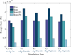 |
Fig. 1 Histograms of oxygen ion escape rates in different simulation runs. The dark-purple and dark-cyan bars in each run refer to the escape rates of exospheric and ionospheric oxygen ions, respectively. The cadet-blue and sky-blue bars in each run denote the ionospheric oxygen ion escape rates originating from the dayside (“D”) and night-side (“N”) ionospheric source regions, respectively. |
3 Simulation results
Figure 1 compares the oxygen ion escape rates among different simulation runs. As the legend shows, the color bars represent the ion escape rates of various origins. The dark-purple and dark-cyan bars present the exospheric and ionospheric oxygen ion escape rates, and the contributions from dayside and nightside ionospheric source regions are further separated by the cadet-blue and sky-blue bars, respectively. Here, the escape rates are calculated by dividing the numbers of escaping oxygen ions of different origins during a certain time interval by the time interval length. Note that, although the escape rates generally vary with time, the present study focuses on the simulation results at the simulation time of 400 s. This is after the simulations have all reached the quasi-steady phase and the simulation results no longer change significantly.
To better visualize the oxygen ion escape paths, Figure 2 illustrates the distribution of the oxygen ion flux in the XZ plane, averaged over −1.6 RM ≤ Y ≤ 1.6 RM, for the different simulation runs as labeled. The overlaid white arrows indicate the direction of the ionospheric oxygen ion flux, with arrow lengths proportional to the flux magnitude. To identify exact regions where the crustal fields influence the ionospheric oxygen ion escape, Figure 3 presents the distribution of the oxygen escape fluxes at the source region, calculated using Equation (1) as described in Section 2.2. While the first row in Figure 3 shows the absolute escape fluxes in the two Group A simulations (no crustal fields), the second and third rows illustrate the relative fluxes for the simulations in Groups B and C, defined as the flux difference with respect to the corresponding simulation in Group A under the same IMF condition.
It should be clarified that the escape rates in the two Group A simulations are identical, so only one set of bars is shown for Runs A1 and A2 in Figure 1. The two Group A simulations have no crustal fields and are under +BY IMF and −BY IMF conditions, respectively. Subsequently, the motional electric field in the solar wind has equal magnitudes but opposite directions in the two simulations, yielding ion escape patterns symmetric about the Z = 0 plane, as seen in Figures 2a and b. Furthermore, nearly all escaping ions in the Group A simulations originate from the dayside ionosphere (Figure 1) and escape through the ion plume over the +E hemisphere, where the solar wind motional electric field points away from Mars (Figures 2a and b) – consistent with the top row in Figure 3.
Comparing the oxygen ion escape rates of the Group B and C simulations with those of Group A (Figure 1), it is clear that the presence of crustal fields enhances the escape rate of ionospheric oxygen ions, particularly under the +BY IMF condition. The total escape rates of ionospheric oxygen ions increase by 8.5 × 10²³ s−1 (+63%), 5.9 × 10²³ s−1 (+40%), 9.2 × 10²³ s−1 (+65%), and 5.1 × 10²³ s−1 (+39%) in Runs B1, B2, C1, and C2, respectively, relative to those in Group A. Moreover, this enhancement is predominantly contributed by ions from the dayside ionosphere, although the contribution of ions from the nightside ionosphere is also substantial. Specifically, the dayside ionospheric oxygen ion escape rates increase by 6.3 × 10²³ s−1 (+56%), 3.3 × 10²³ s−1 (+30%), 6.0 × 10²³ s−1 (+54%), and 3.4 × 10²³ s−1 (+31%), while the corresponding nightside rates increase by 1.9 × 10²³ s−1 (+85%), 2.5 × 10²³ s−1 (+113%), 2.4 × 10²³ s−1 (+109%), and 1.6 × 10²³ s−1 (+72%) for Runs B1, B2, C1, and C2, respectively. These can be clearly seen in Figure 3 as well. On the other hand, the escape rate of exospheric oxygen ions remains largely unchanged across all runs, implying that the influence of crustal fields is mostly confined to low altitudes. As mentioned in Section 2, exospheric ions are produced via photoionization over an extended altitude range, reducing their sensitivity to relatively localized crustal field structures at low altitudes.
Further comparison between Runs B1 and B2 in Figure 1 reveals a higher ionospheric oxygen ion escape rate in Run B1, despite both simulations having the strongest crustal fields on the dayside. On the other hand, Run B2 yields a higher ionospheric oxygen ion escape rate than Run C2, which shares the same IMF condition as Run B2 but has nightside crustal fields. These results suggest that the impact of crustal fields on ion escape is not only determined by the crustal field location but also modulated by the IMF orientation. Moreover, the higher ionospheric oxygen ion escape rate in Run B1 (with respect to Run B2) arises mainly from dayside ions, whereas the lower ionospheric oxygen ion escape rate in Run C2 (in comparison with Run B2) relates mostly to nightside ions. Thus, the dayside and nightside ionospheric ion escapes respond differently to the crustal fields and IMF orientation.
Different crustal fields induce different regional enhancements in the dayside ionospheric oxygen ion escape. Figures 3c and d demonstrate that strong crustal fields on the dayside in the Group B simulations significantly enhance dayside ion escape from the southern hemisphere. Notably, in Run B1, we observe a pronounced transport of dayside ionospheric oxygen ions toward the nightside, forming a tailward escape pathway (Figure 2c) – consistent with the studies by Dong et al. (2017) and Inui et al. (2019). This escape pathway is absent in Run A1 without the crustal fields, where little ion escape occurs from the southern hemisphere. In Run B2, the oxygen ion escape is enhanced in regions already exhibiting significant ion escape in Run A2 (without crustal fields). While moderate crustal fields on the dayside in the Group C simulations also enhance ion escape substantially, the enhancement is concentrated over the +E hemisphere, as seen in Figures 3e and f. Interestingly, regions of enhanced oxygen ion escape flux appear on two sides of the sub-solar longitude (at noon) and extend toward the equator in Runs C1 and C2, consistent with the finding in Ramstad et al. (2016).
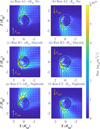 |
Fig. 2 Oxygen ion flux distributions in the XZ plane for different simulation runs, averaged over −1.6 RM ≤ Y ≤ 1.6 RM. In each panel, the black circle represents Mars, the vertical yellow arrow on the left indicates the direction of the solar wind motional electric field (ESW), and the white arrows indicate the direction of the ionospheric oxygen ion flux, with arrow lengths proportional to the flux magnitude. |
4 Discussion
To elucidate the mechanisms by which the crustal fields enhance the ionospheric oxygen ion escape, Figures 4 and 5 present the distributions of the oxygen ion number density and radial component of the bulk velocity (vr) – the two key factors determining the ion escape flux – at an altitude of 450 km, for different simulation runs as labeled. This altitude, 50 km above the ionospheric source region, was chosen to characterize the ion properties after initial acceleration, thereby enabling a proper assessment of the crustal fields’ influence on the early-stage transport of ionospheric oxygen ions. It is worth mentioning that the results remain qualitatively unchanged at higher altitudes, provided the altitude does not differ dramatically from 450 km. It can be seen from Figure 4 that the ion density increases in regions coinciding with the crustal fields on the dayside in the simulations of Groups B and C in comparison with Runs A1 and A2. Based on the quasi-neutrality condition, this result is consistent with MAVEN observations of a 25–30% enhancement in electron density in the same regions (Flynn et al. 2017). On the other hand, the outward vr also show significant enhancements within the crustal field regions in the Group B and Group C simulations compared to Group A (Figure 5). These enhancements result in increased escape fluxes (Figure 3) and higher escape rates (Figure 1) in the Group B and Group C simulations. They can be attributed to modifications of local electric and magnetic field structures induced by the crustal fields, as oxygen ion transport is governed by both magnetic and electric fields. Subsequent analysis investigates how crustal fields modulate the ion escape rate by altering the number density and vr, with emphasis on the role of dayside crustal fields in facilitating ion escape from the ionospheric source region.
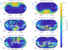 |
Fig. 3 Distributions of the ionospheric oxygen ion escape fluxes in (a) Run A1, (b) Run A2, and the relative escape fluxes in (c) Run B1, (d) Run B2, (e) Run C1, and (f) Run C2 at the source region 400 km above the Martian surface. The solid white curves in each panel are contour lines of the crustal magnetic fields with a magnitude of 40 nT at the same altitude, and the vertical blue vector on the left shows the direction of the solar wind motional electric field (ESW). |
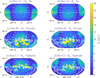 |
Fig. 4 Number density of ionospheric oxygen ions in (a) Run A1, (b) Run A2, (c) Run B1, (d) Run B2, (e) Run C1, and (f) Run C2 at an altitude of 450 km. The solid white curves in each panel are contour lines of the crustal magnetic fields with a magnitude of 40 nT at 400 km, and the vertical blue vector on the left indicates the direction of the solar wind motional electric field (ESW). |
4.1 Influence of magnetic field topology
The crustal fields directly modify the magnetic field topology, thereby influencing ion trajectories. Figure 6 shows the inclination angle value of the magnetic fields in Runs A1, B1, and C1 at an altitude of 450 km. Since Runs A2, B2, and C2 exhibit similar patterns as Runs A1, B1, and C1 in their respective simulation groups, they are not shown for brevity. The 0° and 90° angles indicate that the magnetic field line is tangential and normal to the Martian surface, respectively. In the absence of the crustal fields (Group A), the induced magnetosphere is shaped by the draped IMF and exhibits small dayside magnetic inclination angles, indicating that magnetic field lines lie nearly parallel to the Martian surface. With the inclusion of the crustal fields, magnetic inclination angles in the crustal field regions increase significantly, consistent with Li et al. (2022). This implies that at low altitudes, the magnetic configuration in the crustal field regions is predominantly governed by the crustal fields themselves rather than the draped IMF. The enhanced magnetic inclination and increased field strength reduce the oxygen ion gyroradius and promote field-aligned ion motion. Consequently, a higher fraction of ions are transported outward along magnetic field lines rather than being absorbed by the inner boundary. This leads to localized enhancements in oxygen ion density and outward vr (Figures 4 and 5), in agreement with MAVEN observations (Figure 1 of Fan et al. 2020) and previous simulations (Figure 1 of Li et al. 2022). Therefore, the crustal fields effectively facilitate the outward field-aligned transport of ionospheric oxygen ions, providing an enhanced source population for ion escape.
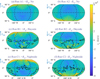 |
Fig. 5 Radial velocity (vr) of ionospheric oxygen ions in (a) Run A1, (b) Run A2, (c) Run B1, (d) Run B2, (e) Run C1, and (f) Run C2 at an altitude of 450 km. The solid black curves in each panel are contour lines of the crustal magnetic fields with a magnitude of 40 nT at 400 km, and the vertical blue vector on the left indicates the direction of the solar wind motional electric field (ESW). |
 |
Fig. 6 Inclination angle of the magnetic field at an altitude of 450 km in (a) Run A1, (b) Run B1, and (c) Run C1. The solid white curves in each panel are contour lines of the crustal magnetic fields with a magnitude of 40 nT at an altitude of 400 km. |
4.2 Electric field effect
The dayside crustal fields also modulate the local electric field environment through their interaction with the solar wind, further influencing oxygen ion dynamics. Figure 7 displays the distribution of the radial electric field (Er) at a 450 km altitude for each run. It is worth clarifying again that the RHybrid simulation platform does not contain a self-consistent description of the ionosphere, and the electric field analyzed here is in the top-side ionosphere above the inner boundary at a 400 km altitude where the ionospheric ions are injected. In the Group B simulations, the magnetic pressure of the crustal fields on the dayside causes the bow shock to stand off at higher altitudes than in the Group A simulations without crustal fields (not shown). This leads to greater plasma deceleration and a reduction in the low-altitude Er magnitude in the strong crustal field region (encircled by the solid black curves on the dayside in Figures 7c and d). In Run B1, although Er points inward within the strong crustal field region, its magnitude is reduced, allowing more ionospheric oxygen ion escape there than in Run A1 (see Figures 3a and c). This effect adds to the crustal field’s influence on the magnetic field topology (as discussed in Section 4.1), causing the most significant increase in oxygen ion escape rate in Run B1. In Run B2, Er points outward and is also weakened within the strong dayside crustal field region (Figure 7d) compared to Run A2 (Figure 7b). This should lead to reduced outward ion transport. However, the dayside ionospheric ion escape rate is much higher in Run B2 than in Run A2, indicating that the magnetic field topology change discussed in Section 4.1 overcomes the weakened Er effect. Finally, in the Group C simulations, the reduction of Er by the moderate crustal fields on the dayside is not as pronounced as that in the Group B simulations. Consequently, the magnetic field topology change (i.e., increased magnetic inclination and magnitude) in dayside crustal field regions causes the locally enhanced oxygen ion density (Figures 4e and f) and outward vr (Figures 5e and 5f), thus increasing ion escape over the +E hemisphere (Figures 2 and 3).
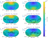 |
Fig. 7 Radial component of the electric field (Er) in (a) Run A1, (b) Run A2, (c) Run B1, (d) Run B2, (e) Run C1, and (f) Run C2 at a 450 km altitude. The solid black curves in each panel are contour lines of the crustal magnetic fields with a magnitude of 40 nT at a 400 km altitude, and the vertical blue vector on the left indicates the direction of the solar wind motional electric field (ESW). |
5 Conclusions
This study employs the 3D global hybrid model RHybrid, combined with escaping ion trajectory tracing to investigate the influence of the crustal magnetic fields on the escape of Martian ionospheric oxygen ions. The results demonstrate that the crustal magnetic fields increase the total oxygen ion escape rate compared to cases without the crustal fields. This enhancement is primarily associated with ionospheric oxygen ions, whereas the escape rate of exospheric oxygen ions remains relatively unaffected by the presence (and location) of the crustal fields, highlighting the altitude-limited influence of the crustal fields on oxygen ion escape. The crustal magnetic fields change the ionospheric oxygen ion escape by modifying the local electric and magnetic field structures. First, they increase the local magnetic inclination and strength, thereby enhancing ion density and outward transport. Second, they reduce the radial component of the local electric field, which further affects ion acceleration and escape. The local magnetic field topology change (the steep magnetic inclination and large magnetic strength) constantly enhances the ionospheric oxygen ion escape, whereas the effect of the local electric field reduction varies, depending on the IMF condition. When strong crustal fields are on the dayside, the radial electric field in that region points downward and upward in the southern hemisphere under +BY IMF and −BY IMF conditions, respectively. Thus, electric field reduction facilitates and suppresses the ion escape, respectively. However, since the magnetic field topology change dominates electric field reduction, the ion escape is enhanced under both IMF conditions, even though the escape rate is higher for +BY IMF. In particular, under the +BY IMF condition, these effects combine to enable an efficient dayside-to-nightside ion transport, forming an extended tailward escape pathway. When strong crustal fields are on the nightside, moderate crustal fields on the dayside only weakly reduce the local electric field. Ion escape enhancement then arises mainly from changes in the magnetic field topology over the +E hemisphere.
Acknowledgements
We wish to thank the Finnish Meteorological Institute for providing the RHybrid simulation platform. This work was supported by the National Natural Science Foundation of China (NSFC) grant 42174203. R.J. received funding from the European Research Council (Grant agreement No. 101124960). It was also supported by the Center for Computational Science and Engineering of Southern University of Science and Technology.
References
- Acuña, M. H., Connerney, J. E. P., F., N., et al. 1999, Science, 284, 790 [NASA ADS] [CrossRef] [Google Scholar]
- Brain, D. A., Baker, A. H., Briggs, J., et al. 2010a, GeoRL, 37, L14108 [Google Scholar]
- Brain, D. A., Barabash, S., Boesswetter, A., et al. 2010b, Icarus, 206, 139 [Google Scholar]
- DiBraccio, G. A., Romanelli, N., Bowers, C. F., et al. 2022, GeoRL, 49, e2022GL098007 [Google Scholar]
- Dong, Y., Fang, X., Brain, D. A., et al. 2015, GeoRL, 42, 8942 [Google Scholar]
- Dong, Y., Fang, X., Brain, D. A., et al. 2017, JGR, 122, 4009 [Google Scholar]
- Dubinin, E., Fraenz, M., Pätzold, M., et al. 2020, JGR, 125, e2020JA028010 [Google Scholar]
- Dubinin, E., Fraenz, M., Pätzold, M., et al. 2023a, GeoRL, 50, e2022GL102324 [Google Scholar]
- Dubinin, E., Fraenz, M., Pätzold, M., et al. 2023b, JGR, 128, e2022JA030575 [Google Scholar]
- Egan, H., Jarvinen, R., Ma, Y., et al. 2019, MNRAS, 488, 2 [Google Scholar]
- Fan, K., Fraenz, M., Wei, Y., et al. 2019, GeoRL, 46, 11764 [Google Scholar]
- Fan, K., Fraenz, M., Wei, Y., et al. 2020, ApJ, 898, L54 [Google Scholar]
- Fang, X., Ma, Y., Brain, D., et al. 2015, JGR, 120, 10 [Google Scholar]
- Fang, X., Ma, Y., Masunaga, K., et al. 2017, JGR, 122, 4117 [Google Scholar]
- Flynn, C. L., Vogt, M. F., Withers, P., et al. 2017, GeoRL, 44, 10812 [Google Scholar]
- Gao, J. W., Rong, Z. J., Klinger, L., et al. 2021, Earth Space Sci., 8, e2021EA001860 [Google Scholar]
- Garnier, P., Jacquey, C., Gendre, X., et al. 2022, JGR, 127, e2021JA030146 [Google Scholar]
- Hanley, K. G., Fowler, C. M., McFadden, J. P., et al. 2022, GeoRL, 49, e2022GL100182 [Google Scholar]
- Hara, T., Huang, Z., Mitchell, D. L., et al. 2022, JGR, 127, e2021JA029867 [Google Scholar]
- Harada, Y., Halekas, J. S., McFadden, J. P., et al. 2015, GeoRL, 42, 8838 [Google Scholar]
- Inui, S., Seki, K., Sakai, S., et al. 2019, JGR, 124, 5482 [Google Scholar]
- Jakosky, B. M., Brain, D., Chaffin, M., et al. 2018, Icarus, 315, 146 [NASA ADS] [CrossRef] [Google Scholar]
- Jarvinen, R., Kallio, E., Janhunen, P., et al. 2009, Ann. Geophys., 27, 4333 [Google Scholar]
- Jarvinen, R., Brain, D. A., Modolo, R., et al. 2018, JGR, 123, 1678 [Google Scholar]
- Jarvinen, R., Kallio, E., & Pulkkinen, T. I. 2022, JGR, 127, e2021JA030078 [Google Scholar]
- Kallio, E., & Barabash, S. 2012, Earth Planets Space, 64, 149 [Google Scholar]
- Kallio, E., & Janhunen, P. 2002, JGR, 107, 1035 [Google Scholar]
- Kallio, E., & Janhunen, P. 2003, Ann. Geophys., 21, 2133 [NASA ADS] [CrossRef] [Google Scholar]
- Kallio, E., Fedorov, A., Budnik, E., et al. 2006, Icarus, 182, 350 [NASA ADS] [CrossRef] [Google Scholar]
- Kallio, E., Fedorov, A., Budnik, E., et al. 2008, Planet. Space Sci., 56, 1204 [NASA ADS] [CrossRef] [Google Scholar]
- Kallio, E., Liu, K., Jarvinen, R., et al. 2010, Icarus, 206, 152 [Google Scholar]
- Li, S., Lu, H., Cui, J., et al. 2020, EPP, 4, 1 [Google Scholar]
- Li, S., Lu, H., Cao, J., et al. 2022, ApJ, 931, 30 [Google Scholar]
- Li, G., Lu, H., Li, Y., et al. 2023, Front. Astron. Space Sci., 10, 0 [Google Scholar]
- Liu, D., Rong, Z., Gao, J., et al. 2021, ApJ, 911, 113 [NASA ADS] [CrossRef] [Google Scholar]
- Ma, Y. J., & Nagy, A. F. 2007, GeoRL, 34, L08201 [Google Scholar]
- Man, H., Xu, X., Yang, P., et al. 2025, Phys. Fluids, 37 [Google Scholar]
- Nilsson, H., Edberg, N. J. T., Stenberg, G., et al. 2011, Icarus, 215, 475 [NASA ADS] [CrossRef] [Google Scholar]
- Ramstad, R., Barabash, S., Futaana, Y., et al. 2016, GeoRL, 43, 10 [Google Scholar]
- Romanelli, N., Modolo, R., Leblanc, F., et al. 2018, JGR, 123, 5315 [Google Scholar]
- Sakata, R., Seki, K., Sakai, S., et al. 2022, JGR, 127, e2022JA030427 [Google Scholar]
- Wang, M., Xu, X., Lee, L. C., et al. 2022, A&A, 667, A41 [NASA ADS] [CrossRef] [EDP Sciences] [Google Scholar]
- Wang, M., Guan, Z., Xie, L., et al. 2024, JGR, 129, e2024JA032806 [Google Scholar]
- Weber, T., Brain, D., Xu, S., et al. 2021, JGR, 126, e2021JA029234 [Google Scholar]
- Wei, Y., Pu, Z., Zong, Q., et al. 2014, Earth Planet. Sci. Lett., 394, 94 [Google Scholar]
- Xu, S., Luhmann, J. G., Mitchell, D. L., et al. 2023, ApJ, 957, L29 [Google Scholar]
- Zhang, C., Rong, Z., Nilsson, H., et al. 2021, ApJ, 922, L33 [Google Scholar]
- Zhou, J., Liu, K., Jarvinen, R., et al. 2024, ApJ, 976, 7 [Google Scholar]
All Tables
All Figures
|
Fig. 1 Histograms of oxygen ion escape rates in different simulation runs. The dark-purple and dark-cyan bars in each run refer to the escape rates of exospheric and ionospheric oxygen ions, respectively. The cadet-blue and sky-blue bars in each run denote the ionospheric oxygen ion escape rates originating from the dayside (“D”) and night-side (“N”) ionospheric source regions, respectively. |
| In the text | |
|
Fig. 2 Oxygen ion flux distributions in the XZ plane for different simulation runs, averaged over −1.6 RM ≤ Y ≤ 1.6 RM. In each panel, the black circle represents Mars, the vertical yellow arrow on the left indicates the direction of the solar wind motional electric field (ESW), and the white arrows indicate the direction of the ionospheric oxygen ion flux, with arrow lengths proportional to the flux magnitude. |
| In the text | |
|
Fig. 3 Distributions of the ionospheric oxygen ion escape fluxes in (a) Run A1, (b) Run A2, and the relative escape fluxes in (c) Run B1, (d) Run B2, (e) Run C1, and (f) Run C2 at the source region 400 km above the Martian surface. The solid white curves in each panel are contour lines of the crustal magnetic fields with a magnitude of 40 nT at the same altitude, and the vertical blue vector on the left shows the direction of the solar wind motional electric field (ESW). |
| In the text | |
|
Fig. 4 Number density of ionospheric oxygen ions in (a) Run A1, (b) Run A2, (c) Run B1, (d) Run B2, (e) Run C1, and (f) Run C2 at an altitude of 450 km. The solid white curves in each panel are contour lines of the crustal magnetic fields with a magnitude of 40 nT at 400 km, and the vertical blue vector on the left indicates the direction of the solar wind motional electric field (ESW). |
| In the text | |
|
Fig. 5 Radial velocity (vr) of ionospheric oxygen ions in (a) Run A1, (b) Run A2, (c) Run B1, (d) Run B2, (e) Run C1, and (f) Run C2 at an altitude of 450 km. The solid black curves in each panel are contour lines of the crustal magnetic fields with a magnitude of 40 nT at 400 km, and the vertical blue vector on the left indicates the direction of the solar wind motional electric field (ESW). |
| In the text | |
|
Fig. 6 Inclination angle of the magnetic field at an altitude of 450 km in (a) Run A1, (b) Run B1, and (c) Run C1. The solid white curves in each panel are contour lines of the crustal magnetic fields with a magnitude of 40 nT at an altitude of 400 km. |
| In the text | |
|
Fig. 7 Radial component of the electric field (Er) in (a) Run A1, (b) Run A2, (c) Run B1, (d) Run B2, (e) Run C1, and (f) Run C2 at a 450 km altitude. The solid black curves in each panel are contour lines of the crustal magnetic fields with a magnitude of 40 nT at a 400 km altitude, and the vertical blue vector on the left indicates the direction of the solar wind motional electric field (ESW). |
| In the text | |
Current usage metrics show cumulative count of Article Views (full-text article views including HTML views, PDF and ePub downloads, according to the available data) and Abstracts Views on Vision4Press platform.
Data correspond to usage on the plateform after 2015. The current usage metrics is available 48-96 hours after online publication and is updated daily on week days.
Initial download of the metrics may take a while.