| Issue |
A&A
Volume 706, February 2026
|
|
|---|---|---|
| Article Number | A109 | |
| Number of page(s) | 8 | |
| Section | Planets, planetary systems, and small bodies | |
| DOI | https://doi.org/10.1051/0004-6361/202556819 | |
| Published online | 05 February 2026 | |
Juno radio occultations reveal the structure of Jupiter's cold northern polar vortex
1
Department of Earth and Planetary Sciences, Weizmann Institute of Science,
Rehovot
76100,
Israel
2
School of Physics and Astronomy, University of Leicester,
Leicester,
UK
3
Jet Propulsion Laboratory, California Institute of Technology,
Pasadena,
CA,
USA
4
Department of Industrial Engineering, University of Bologna,
Forlì,
Italy
5
School of Electrical and Computer Engineering, Georgia Institute of Technology,
Atlanta,
GA,
USA
6
Southwest Research Institute,
San Antonio,
TX,
USA
★ Corresponding authors: This email address is being protected from spambots. You need JavaScript enabled to view it.
; This email address is being protected from spambots. You need JavaScript enabled to view it.
Received:
11
August
2025
Accepted:
29
November
2025
Abstract
Context. Jupiter’s polar upper troposphere and stratosphere host a persistent cold vortex poleward of 65°N, but its detailed structure and dynamics have remained difficult to resolve.
Aims. The goal is to characterize the thermal structure and dynamics of the polar vortex using new and complementary remote sensing techniques.
Methods. We used a combination of high-resolution vertical profiles derived from Juno’s recent radio occultation measurements and mid-infrared imaging from the VLT/VISIR instrument. The former provided direct retrievals of temperature and density near and within the vortex, while VISIR imaging revealed spatial thermal contrasts across the region.
Results. Our analysis confirms the presence of a steep meridional temperature jump at 65°N, of about 7±1 K at 100 mbar, which is consistent with a strong vertical wind shear and a prograde polar stratospheric jet reaching up to 80 ms−1 at the 10 mbar level. We find the atmosphere to be thermally stable above 0.55 bar, reaching a Brunt-Väisälä frequency of 0.025 s−1 in the mid-stratosphere. Thermal contrasts observed in the infrared data align with the vertical structures inferred from radio occultations, which validates the presence and extent of the cold vortex.
Conclusions. These findings offer a quantitative analysis of the thermal structure and the dynamical behavior of Jupiter’s polar atmosphere and demonstrate the diagnostic power of combining radio occultation and thermal infrared techniques in planetary atmospheric studies.
Key words: methods: observational / planets and satellites: atmospheres / planets and satellites: gaseous planets / planets and satellites: individual: Jupiter
© The Authors 2026
 Open Access article, published by EDP Sciences, under the terms of the Creative Commons Attribution License (https://creativecommons.org/licenses/by/4.0), which permits unrestricted use, distribution, and reproduction in any medium, provided the original work is properly cited.
This article is published in open access under the Subscribe to Open model. This email address is being protected from spambots. You need JavaScript enabled to view it. to support open access publication.
1 Introduction
Jupiter’s polar atmosphere is a dynamic and complex region influenced by strong zonal jets, vertical wind shear, auroral processes, and radiative effects associated with unique polar aerosols (Hue et al. 2024). The cold vortex in Jupiter’s northern polar atmosphere has been detected through a combination of ground-based and space-based observations (Flasar et al. 2004; Simon-Miller et al. 2006; Nixon et al. 2010; Fletcher et al. 2016; Orton et al. 2022; Bardet et al. 2024). A similar cold vortex is seen in the southern hemisphere of the planet, explored most recently using the Mid-Infrared Instrument measurements (MIRI) on the James Webb Space Telescope (JWST) (Rodríguez-Ovalle et al. 2024). While both poles are of significant interest, this study focuses on the northern hemisphere, where a persistent cold polar vortex dominates the upper troposphere and lower stratosphere. On Earth, a well-known example of a cold-core polar vortex forms over Antarctica during the southern winter, where strong circumpolar winds trap cold air in the stratosphere, leading to unique seasonal and chemical effects (Andrews et al. 1987; Waugh & Randel 1999).
Fletcher et al. (2016) used Cassini’s Composite Infrared Spectrometer (CIRS) to identify sharp temperature drops in the high latitude regions, which they interpreted as evidence of cold polar vortices accompanied by positive vertical shear on prograde jets. These features were mapped at high resolution in the mid-infrared using ESO’s Very Large Telescope (VLT) Imager and Spectrometer for mid-Infrared (VISIR) and the Texas Echelon Cross Echelle Spectrograph (TEXES) on NASA’s IRTF, poleward of 64°N. The results are consistent with sustained radiative cooling (Lacy et al. 2002; Bardet et al. 2024). The cold vortex in the troposphere is readily visible in mid-infrared imaging sounding the hydrogen-helium collision-induced absorption. However, in the stratosphere the presence of the northern cold vortex is clearest during intervals of minimal auroral heating when the absence of significant high-latitude energy input from charged particles allows clearer thermal contrasts to be detected (Porco et al. 2003; Fletcher et al. 2016; Bardet et al. 2024). The vortex’s cooling appears consistent with the presence of high-latitude, optically thick aerosols, which become vertically extensive above ~65° latitude and are readily visible in visible-near-IR imaging (Barrado-Izagirre et al. 2008). These aerosols likely enhance radiative cooling (Zhang et al. 2013), but their distribution appears asymmetric between the poles. The southern cold vortex is well aligned with the auroral oval and associated aerosols, whereas in the north the auroral oval extends well beyond the vortex, potentially allowing aerosols to disperse and weakening the correlation between haze and temperature structure (Guerlet et al. 2020; Bardet et al. 2024). The polar boundary exhibits longitudinal meandering, potentially influenced by a Rossby wave (Li et al. 2004; Barrado-Izagirre et al. 2008), as seen in JunoCam visible-light observations (Orton et al. 2017; Rogers et al. 2022). The polar vortex described here is distinct from the circumpolar cyclones (CPCs) and polar cyclones (PCs) identified poleward of 83°N (Adriani et al. 2018; Gavriel & Kaspi 2021); rather, these smaller-scale cyclonic structures appear to be embedded within the broader, overarching polar vortex system.
Despite significant progress in identifying the vortex and its lateral extent, many questions remain about its vertical structure, the velocity of its winds, and precise thermal gradients (Flasar et al. 2004). Infrared imaging techniques primarily offer relative temperature contrasts and lack the vertical resolution to resolve detailed stratification. Furthermore, infrared spectroscopy potentially suffers from degeneracies between temperature, composition, and aerosol opacity; published temperature gradients assume that these degeneracies have been successfully accounted for, which is particularly challenging at high emission angles in the polar domain.
To address this gap, we employed new radio occultation measurements from NASA’s Juno mission (Bolton et al. 2017). Radio occultation (RO) is a remote sensing technique that retrieves atmospheric pressure, temperature, and density profiles with high vertical resolution by analyzing how radio signals are bent as they pass through a planet’s atmosphere (Schinder et al. 2011, 2015). Although not included in Juno’s prime mission science plan, these experiments were incorporated during the mission’s extended phase (Smirnova et al. 2025), when the spacecraft’s orientation during close approaches to Jupiter allowed Earth-pointed radio signals to traverse its atmosphere. This study uses radio occultation data from perijoves 64 through 72 (August 2024 to May 2025), a period during which several ingress occultations intersected the cold northern vortex. These new observations represent an unprecedented opportunity to derive absolute temperature profiles within and immediately outside the northern polar vortex at high vertical resolution, marking the first time any mission has obtained such detailed measurements of Jupiter’s northern polar stratosphere via radio occultations.
The mid-infrared context for this study is provided by data acquired with the VISIR instrument (Lagage et al. 2004; Fletcher et al. 2009). These data were obtained on 16 October 2024 and offer exceptionally high spatial resolution and captured longitudes that were not obscured by auroral heating. The VLT data highlight thermal contrasts across Jupiter’s polar region and are used here to place the radio occultation tracks in their broader thermal context. The VLT observations were conducted one week before Juno’s 66th perijove, which allowed for near-simultaneous infrared and radio analysis.
In this study, we present an integrated view of Jupiter’s northern cold polar vortex using both techniques: direct measurement via radio occultations and indirect measurement with remote sensing. Section 2 describes the radio occultation and VLT dataset and retrieval methods. Section 3 presents temperature profiles and gradients derived from the RO data. In Sect. 4 we discuss the implications for polar atmospheric dynamics.
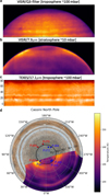 |
Fig. 1 Several perspectives of the northern polar vortex. Panel a: VLT/VISIR image from 16 October 2024 that illustrates the colder polar vortex in the Q3 filter (tropospheric measurements at 19.5 μm around 100 mbar). Panel b: VLT/VISIR image from 16 October 2024 that illustrates the colder polar vortex in the 7.9 μm-filter (stratospheric measurements around 10 mbar). Panel: TEXES image from 28 February 2025 that illustrates the colder polar vortex in the 17.1 μm (586 cm−1) wavelength (tropospheric observations around 100 mbar). The composite polar projection in panel d of Jupiter’s north pole combines the VLT/VISIR 7.9 μm infrared map (panel b), where the brightness temperatures are between 142.8 K and 151.9 K, with Cassini background imagery [Credit: NASA/JPL/Space Science Institute (2006)]. The dashed black circle serves as a visual marker for the 65° planetocentric latitude. Ingress locations of Juno radio occultations from PJ64-PJ72 are overlaid. Occultation points are color-coded by whether they intersect the cold polar vortex (blue) or surrounding region (red). Details on the RO experiments can be found in Table A.1. |
2 Data and methods
The presence of a cold vortex in Jupiter’s northern polar atmosphere has been identified through both ground-based observations (Fletcher et al. 2016; Bardet et al. 2024) and space-borne instruments (Flasar et al. 2004; Simon-Miller et al. 2006). The most recent detections of this thermal anomaly come from mid-infrared measurements, including TEXES spectroscopy (Lacy et al. 2002) and high-resolution imaging from VISIR on the VLT (Lagage et al. 2004). Figure 1 shows the composite polar projection of Jupiter’s north pole. The polar map was made from the Cassini spacecraft (Matson et al. 2002; NASA/JPL/Space Science Institute 2006).
Figure 1 shows the infrared observations, including a global map of Jupiter captured on 16 October 2024 using the Q3 filter (Figs. 1a and Id), which is sensitive to hydrogen-helium collision-induced absorption from the upper troposphere at 19.5 μm (Fletcher et al. 2009). Figure 1b shows the 7.9 μm image, which captures the methane emission taken at the stratospheric altitudes around 10 mbar. The exceptional diffractionlimited spatial resolution of the VLT enables the detection of fine thermal contrasts in Jupiter’s mid-latitudes and polar regions, features that were not resolvable by earlier missions such as Voyager and Cassini (Bardet et al. 2024), nor by groundbased facilities with smaller apertures like the IRTF (TEXES image in Fig. 1c; Fletcher et al. 2016). These observations were obtained in close temporal proximity to Juno’s 66th perijove on 22 October 2024, which offers a unique opportunity to correlate high-resolution ground-based mid-infrared maps with radio occultation experiments from the spacecraft, particularly over Jupiter’s polar domains.
Recent radio occultations, conducted since August 2024 (Table A.1), offer a detailed exploration of Jupiter’s northern polar region. Figure 1d shows the locations of these ingress occultations between PJ64-PJ72 (PJ71 is excluded due to an unsuccessful RO experiment). We analyzed these radio occultations to investigate the thermal structure within the colder polar vortex region (above 65° latitude - PJ64 until PJ67 and PJ72) and outside of this region (slightly below 65° latitude - PJ68 until PJ70). These profiles quantify the vertical extent, temperature gradients, and broader dynamical context of the polar vortex.
Radio occultation measurements with the Juno spacecraft rely on coherent radio links at X-band (8.4 GHz) and Ka-band (32 GHz), which are transmitted toward Earth as Juno passes behind Jupiter relative to the Deep Space Network (DSN). Since radio occultation was not a baseline science objective during the mission’s initial planning, Juno was not equipped with an ultrastable oscillator (USO; Buccino et al. 2023). As a result, all occultation experiments are carried out in a twoway mode, where a frequency-stable uplink signal is transmitted from Earth in the X-band and translated onboard to generate coherent downlinks in both bands. This configuration enables dual-frequency analysis to reduce ionospheric effects and isolate the neutral atmospheric contribution of approximately the 1-500 mbar region (Hubbard et al. 1975; Hubbard et al. 1995; Caruso et al. 2025). One limitation of Juno’s occultation geometry is the fixed pointing of its high-gain antenna during each flyby. Juno maintains a static pointing solution, which can lead to off-axis beam losses, particularly near egress, that potentially affect signal quality and limit the depth probed in the atmosphere to ~0.5 bar (Buccino et al. 2023).
In this analysis, we applied a two-way 3D numerical ray tracing method following the approaches outlined by Schinder et al. (2015) and Caruso et al. (2025). The radio signal data were acquired by the DSN open-loop receiver (OLR), sampled in open-loop mode at rates ranging from 16 to 100 kHz. We performed the frequency retrieval at intervals of 0.1 or 0.25 seconds using either fast Fourier transform (FFT; Togni et al. 2025) or phase-locked loop (PLL) techniques (Buccino et al. 2018). These observed frequencies were then mixed with known reference frequencies to reconstruct the sky frequency necessary for occultation analysis. To minimize high-frequency
noise and remove residual outliers, we applied a Savitzky-Golay filter in the frequency processing and a moving average filter during the post-processing stage. The total atmospheric potential, which includes both gravitational and centrifugal contributions, is expressed as
![Mathematical equation: \begin{aligned} U= & \frac{G M}{r}\left[-1+J_2 P_2(\sin \theta)\left(\frac{a}{r}\right)^2\right. \\ & \left.+J_4 P_4(\sin \theta)\left(\frac{a}{r}\right)^4+J_6 P_6(\sin \theta)\left(\frac{a}{r}\right)^6\right]+Q, \end{aligned}](/articles/aa/full_html/2026/02/aa56819-25/aa56819-25-eq1.png) (1)
(1)
where GM is Jupiter’s gravitational parameter, r is the radial distance, a is Jupiter’s equatorial radius, Jn are the zonal gravity harmonic coefficients (Durante et al. 2020), Pn are the associated Legendre polynomials, and θ is the planetocentric latitude. We treat the atmosphere as barotropic down to 0.5 bar using this potential, which is consistent with gravity measurements that indicate barotropic flow at and below the cloud level (Kaspi et al. 2018, 2023). The centrifugal component of the potential  , where l = r cos θ is the distance from the axis of rotation and ω is the rotation rate, is precomputed numerically using a wind model of Jupiter (Tollefson et al. 2017). These winds affect the shape of the equipotential surfaces, which, under the barotropic assumption, also define layers of constant density, refractive index n, and refractivity N = n - 1 (Galanti et al. 2023). The refractivity governs the deflection of radio waves as they pass through the atmosphere.
We inferred the structure of the atmosphere via a two-way ray tracing approach (Schinder et al. 2015; Caruso et al. 2025), where signals are traced through an initially unknown atmospheric model. By iteratively adjusting the model to reproduce the observed uplink and downlink frequencies, the method yields a stratified atmospheric profile with known refractivity gradients. To convert these gradients into temperature and pressure, the composition of the atmosphere must be known. We adopted the latest compositional model by Gupta et al. (2022), which has already been applied to update earlier datasets such as the Voyager radio occultation profiles (first shown in Lindal et al. 1981). The atmospheric density ρ was determined from the refractivity using
 (2)
(2)
where mm is the mean molecular mass and κ is the mean refractive volume, using the values for the composition from Gupta et al. (2022, mm = 3.84 × 10⁻²⁷ kg and κ = 4.56 × 10⁻³³ km3). Next, the density was integrated assuming hydrostatic equilibrium, to yield the temperature
 (3)
(3)
where kB is the Boltzmann constant, ρn = N/κ is the number density, and U0 is the potential level of reference at which the upper boundary condition T(U0) is enforced (Caruso et al. 2025). Finally, using the ideal gas law, the pressure was obtained with
 (4)
(4)
The vertical resolution of the retrieved pressure-temperature profiles, shown in Fig. 2a, is governed by the sampling interval used during the data processing. Several factors contribute to the overall uncertainty in these profiles, including signal noise, the choice of upper boundary conditions in the temperature integration, the assumed wind field used in calculating the gravitational potential, and uncertainties in the Juno trajectory (Caruso et al. 2025).
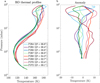 |
Fig. 2 Panel a: pressure-temperature profiles retrieved from eight Juno radio occultation events between PJ64-PJ72, spanning 1-560 mbar. Panel b: same profiles but with the mean subtracted to emphasize deviations relative to the ensemble mean. The deepest pressure shown in the anomalies (195 mbar) corresponds to the shallowest extent of all RO profiles, limited by PJ-67. Details on RO experiments can be found in Table A.1. The measurements come with uncertainties, which are shown in detail at certain levels in Fig. 3 and described in Sect. 2. |
2.1 Upper boundary temperature and error estimates
Uncertainties in radio occultation temperature retrievals arise from several sources, including the choice of the upper boundary condition at 1 mbar, instrumental noise, assumptions about the background wind field, and spacecraft trajectory knowledge. Of these, the boundary condition typically exerts the strongest influence on the retrieved stratospheric temperatures above the 10 mbar level. The choice of the upper boundary temperature is a critical aspect of any temperature retrieval based on radio occultation data, particularly when the upper boundary lies near or above the 1 mbar level, where the atmosphere becomes tenuous and instrumental sensitivity diminishes.
Up to now, approaches to setting the 1 mbar boundary have advanced with observational capabilities and independent constraints. Pioneer 10/11 provided the first glimpses of Jupiter’s stratosphere but with large uncertainties: radio occultation profiles were unreliable above 10 mbar and gave 1 mbar temperatures of 150 ± 40 K (Kliore et al. 1976). Voyager 1/2 radio occultations improved matters by reaching the 1 mbar level with dual-frequency corrections for ionospheric effects and by using mid-infrared measurements from IRIS and contemporaneous constraints, yielding 160 ± 20 K, where the error budget was dominated by uncertainties in He/H2, ephemerides, and instrument noise (Lindal et al. 1981; Simon-Miller et al. 2006). A step change came with Cassini’s 2000 flyby: mid-infrared measurements from CIRS delivered global coverage and robust 1 mbar constraints via optimal estimation, with typical uncertainties of ±3 K (Simon-Miller et al. 2006; Fletcher et al. 2016).
At latitudes within ±10° of each radio occultation point, the CIRS-retrieved temperatures at 1 mbar vary by no more than ±5 K (Fletcher et al. 2016). Accordingly, we adopted the 1 mbar temperature measured by CIRS at the latitude of the occultation event and assigned an uncertainty of ±5 K (performing the inversion at minimum and maximum conditions for each RO experiment). In practice, the upper boundary term dominates the error budget between 1 and 10 mbar, whereas below ~10 mbar the other contributions are dominant. Quantitatively, the propagated uncertainties are ±5 K near 1 mbar, decreasing to ±1.2 K by 10 mbar and to ±1 K at deeper levels (the latter reflecting the non-diminishing 1 K from non-boundary sources). The additional non-diminishing error of 1 K used to account for signal noise, the assumed wind field in the gravitational potential, and Juno trajectory uncertainties follows Caruso et al. (2025). This approach leverages the high precision and spatial resolution of the CIRS measurements and represents a significant refinement over earlier assumptions based on more limited data. Although the temperatures at 1 mbar, measured by CIRS and thus set as the upper boundary for the radio occultation inversions, are higher north of 65 °N and lower to the south, this trend reverses at deeper levels, clearly delineating the boundary of the polar vortex. This reversal provides even stronger evidence for the presence of a cold polar vortex.
The 1 mbar region is particularly interesting, as several stratospheric studies report auroral heating at this pressure level; however, this heating is reported to diminish rapidly with depth (Flasar et al. 2004; Sinclair et al. 2017; Cavalié et al. 2021). Juno performed two auroral occultations (PJ64 and PJ70), but neither revealed significant thermal variations throughout the profile. Because the retrieval upper boundary is fixed at 1 mbar from CIRS, no robust conclusions can be drawn about the precise thermal structure at that level. Although CIRS has shown localized temperature enhancements under the aurora at specific longitudes and latitudes, these features are not evident in the zonal average or the occultation data, limiting our ability to characterize the auroral region’s temperature structure in this work.
3 Results
3.1 Temperature structure
The radio occultation data reveal a clear latitudinal transition in the vertical temperature-pressure structure of Jupiter’s northern polar atmosphere. As illustrated in Fig. 2a, temperature profiles exhibit notable differences depending on whether they were sampled inside or outside the boundary of the northern polar vortex, defined here as latitude 65°N. All latitudinal values referenced in this study correspond to the top of each profile (at 1 mbar) and are expressed in planetocentric coordinates, since the overall change in latitude over the depth of the profile is negligible (~0.5°).
Ingress occultations from Perijoves 64 through 67 and 72 were acquired at higher latitudes, 66.6°, 68.4°, 68.6°, 66.8°N, and 69.1°N, which places them well within the cold vortex region. In contrast, the ingress events at Perijoves 68, 69, and 70 occurred further toward the equator, at 64.3°, 62.7°, and 63.4°N, respectively, outside the vortex boundary. When the ensemble mean is subtracted from each profile, the resulting anomalies, shown in Fig. 2b, highlight relative temperature differences. Positive deviations indicate warmer-than-average conditions, while negative values correspond to cooler anomalies. In the midstratosphere (1-10 mbar), the retrieved temperatures are subject to larger uncertainties than at deeper levels. Moreover, the radio signal in this pressure range can be affected by ionospheric contributions penetrating into the neutral atmosphere. We mitigated these effects using a dual-frequency analysis (X and Ka bands) to recognize and subtract the ionospheric term (Caruso et al. 2025). However, in profiles that lack reliable Ka-band coverage, a residual ionospheric structure may remain. Consequently, temperatures between 1 and 10 mbar are reported for completeness but are not used to infer fine-scale variability; our interpretation in this layer is limited to broad-scale behavior and is reflected in the larger quoted uncertainties.
This analysis clearly demonstrates a consistent thermal contrast between vortex interior and exterior regions, with colder stratification present inside the vortex. Across nearly all pressure levels, temperatures are consistently higher in the lower-latitude profiles, which reaffirms earlier observations shown in Fig. 1 and suggests that degeneracies between temperature, aerosol, and composition were successfully resolved via infrared spectroscopy.
This contrast becomes even more apparent when examining the profiles with the mean removed, as shown in Fig. 2b: positive temperature anomalies align with the profiles located outside the vortex, while negative anomalies are associated with those inside, poleward of 65°N. Figure 3 shows the temperatures at four different levels, 10, 70, 100, and 195 mbar. We observe temperature anomalies of 10 K at the high stratospheric levels around 10 mbar, 8 K at 70 mbar, 7 K at the tropospheric depths around 100 mbar, and 5 K at the 195 mbar level. For each radio occultation profile, the total uncertainty at the different pressure levels is included in Fig. 3. The 1-mbar level is omitted from the figure, since the solution is particularly sensitive to the boundary assumption and can be affected by residual ionospheric contributions. A qualitative comparison of VLT zonal-mean brightness temperatures shows a 2 ± 1 K decline at 7.9 μm (stratosphere) and a 5 ± 1 K decline at 19.5 μm (troposphere) between 62° and 69° latitude, consistent with the values in Fig. 3.
Among the set of profiles, only PJ-66 and PJ-72 ingress extend to greater depths, reaching pressures of ~0.5 bar, while the remaining profiles are notably shallower. This greater vertical extent results from the specific configuration of the radio occultation experiment during those experiments, where the antenna was oriented to maximize Earth visibility, thereby extending the measurement duration. However, this optimization came at the expense of the egress profile in the southern hemisphere, which is correspondingly shallower due to the fixed pointing strategy.
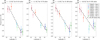 |
Fig. 3 Temperature at four pressure levels (10, 70, 100, and 195 mbar) from each radio occultation profile. Gradient strength across the vortex boundary is quantified and stated in each subplot title. The error bars at each level indicate the total uncertainties comprised from the upper temperature boundary, noise, trajectory uncertainties, and cloud wind considerations (uncertainty estimation description in Sect. 2). |
3.2 Wind shear and zonal velocity estimation
Radio occultation measurements also provide valuable information into the dynamics of Jupiter’s atmosphere. In particular, they enable the estimation of local wind shear, which offers a way to examine the relationship between the vertical thermal structure and zonal wind patterns above the cloud tops. Mid-infrared spectroscopy lacks sensitivity at the ~20 to ~80 mbar range, which leaves a critical gap in our understanding of the lower stratosphere; the direct vertical profiles obtained here therefore provide the first opportunity to quantify wind shear in this region with high precision. To estimate the zonal wind velocity at Jupiter’s northern polar region, we applied thermal wind balance, which relates vertical wind shear to meridional temperature gradients for rapidly rotating planets. The vertical wind shear is determined via the thermal wind equation
 (5)
(5)
where f is the Coriolis parameter,  is the meridional temperature gradient, and T is the average temperature at a specific level. Using this formulation, we calculated the vertical shear of the zonal wind across the northern polar vortex (~65°N). Our results (Fig. 4a) show a strong positive shear at the 10 mbar level, with values around 0.85 m s−1 per kilometer of altitude and at the 70 to 100 mbar level, with values around 0.4 m s−1 per kilometer of altitude. At deeper pressure levels, near 195 mbar, we see weaker shear with values around 0.25 m s−1 per kilometer of altitude. The total uncertainty at different pressure levels (included in Fig. 3) is propagated into the uncertainties of the stratospheric jet velocities in Fig. 4.
To derive the zonal wind profile, pressure levels were converted to altitudes and the wind velocities at each level were computed by integrating the shear from the cloud level at 700 mbar, where the representative observed wind (at ~65°N planetocentric) is 30 m s−1 (Tollefson et al. 2017; Hueso et al. 2023), to the upper pressure level of 10 mbar. This layer-based approach enabled us to estimate the vertical structure of the zonal wind across multiple pressure levels, revealing a wind velocity of approximately 80±12ms−1 at 10 mbar (Fig. 4b). This implies a stratospheric circumpolar jet stream reaching velocities of ~80 ms−1.
The high-resolution temperature profile (Fig. 4c) permits the computation of the atmospheric stability, presented here as the Brunt-Väisälä (buoyancy) frequency N. Across the depth of the radio occultations, values reach as high as N ≈ 2.5 × 10⁻² s−1 in the lower stratosphere, decrease toward the upper troposphere, and tend toward 0 as the profile becomes adiabatic at depths of 0.55 bar. These values are consistent with previous work for the lower stratosphere (Watkins & Cho 2013; O’Neill et al. 2017) and the upper troposphere above ~ 1 bar (Magalhães et al. 2002; Lee & Kaspi 2021). These results provide a compelling validation of the thermal wind shear calculations applied to remote sensing data, and yield values that are consistent with those inferred from CIRS and TEXES observations in the earlier analysis by Fletcher et al. (2016) and the more recent one by Bardet et al. (2024).
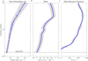 |
Fig. 4 Vertical inferred zonal wind velocity (panel a) and shear (du/dz) profiles (panel b) calculated from the temperature structure using the thermal wind equation. Wind velocities are shown from the cloud tops at 0.7 bar to 10 mbar. The shading indicates the uncertainty envelope, propagated from the temperature inversions (uncertainty estimation description in Sect. 2). Panel c: mean Brunt-Väisälä (buoyancy) frequency (N) in the lower stratosphere and upper troposphere region where the shading indicates the envelope of variability of the individual profiles. |
4 Discussion
The results presented here provide confirmation of the existence and structure of Jupiter’s cold northern polar vortex in the midstratosphere. By combining high-spatial-resolution mid-infrared imaging from VLT/VISIR, which qualitatively reveals the thermal contrasts associated with the polar vortex, with vertical high-resolution temperature profiles from Juno radio occultations, this study provides a comprehensive view of the thermal and dynamical properties of the polar vortex. The VISIR image serves as a visual confirmation of the cold vortex structure, while the radio occultations allow us to quantify the associated temperature differences. The radio occultation profiles reveal temperature gradients near the vortex boundary, with a strong cooling poleward of 65°N, in agreement with previous identifications of the vortex edge in infrared observations (Fletcher et al. 2016; Bardet et al. 2024). The agreement between the VISIR brightness temperature contrasts and the vertical temperature structure derived from occultations confirms that the cold polar anomaly extends vertically through the lower stratosphere, rather than being confined to a narrow altitude range, and that this is often obscured in mid-IR imaging by powerful emissions of methane within the northern auroral oval.
Meridional temperature gradients, via the thermal wind equation, yield the vertical shear ∂u/∂z and indicate a prograde jet with velocities increasing with altitude. The shear peaks near 10 mbar at ~0.85ms−1 km−1, which is consistent with previous studies (Fletcher et al. 2016; Bardet et al. 2024). Integrating the pressure-resolved shear to recover the zonal wind results in a velocity of 80 ± 12ms−1 at 10mbar. Given that cloud-top winds at this latitude (~65°N) are approximately 30ms−1 (Tollefson et al. 2017; Hueso et al. 2023), this suggests the presence of a strong stratospheric circumpolar jet contributing an additional ~50ms−1 above the troposphere. The retrieved wind profile further suggests that the vortex is embedded within a broader eastward jet, which becomes increasingly pronounced with height, consistent with a thermal wind response to high-latitude radiative forcing.
Direct Atacama Large Millimeter Array (ALMA) measurements in the upper stratosphere at ~0.1 mbar (Cavalié et al. 2021) reveal fast prograde jets at high latitudes of about 150 m s−1 near 65°N on the eastern limb, where the sampled location lies outside the northern auroral oval. Our radio-occultation inversions produce meridional gradients that, via thermal-wind balance, imply an increase of zonal wind with altitude. Integrating the inferred shear from 10 mbar upward yields upper-stratospheric wind speeds that are consistent with the ALMA values.
An important implication of these findings is the potential role of high-latitude aerosols in reinforcing the vortex’s cold core. Enhanced aerosol opacity above 65°N has been proposed to increase long-wave radiative cooling (Zhang et al. 2013; Guerlet et al. 2020). The vertical coherence of the cold anomaly observed here supports this interpretation and suggests that aerosols may contribute to maintaining the stratification necessary for strong jet formation and thermal isolation (Bardet et al. 2024). The new vertical temperature profiles also offer critical constraints for models of Jovian polar circulation. In particular, the observed sharp thermal gradients and associated wind shear point to a robust balance between radiative forcing and dynamical adjustment. These data provide valuable benchmarks for future general circulation models that attempt to simulate polar vortex formation and maintenance on gas giants.
While the present analysis focused on the northern hemisphere, future work should apply similar techniques to the south pole, where auroral heating and aerosol opacity differ significantly but a polar vortex is still known to exist and was recently explored using JWST/MIRI (Rodríguez-Ovalle et al. 2024). Looking ahead, radio occultation experiments and retrievals of the temperature and wind spanning Jupiter’s entire stratosphere will be routinely performed with the JUICE (JUpiter ICy moons Explorer) mission to deeper layers and provide critical context for these localized case studies (Fletcher et al. 2023). Additionally, repeated occultations over time may help reveal seasonal changes in the vortex structure. Overall, the integration of Juno occultation data with ground-based mid-infrared observations significantly advances our understanding of Jupiter’s polar stratosphere. The results underscore the importance of combining vertically and horizontally resolved measurements to characterize the dynamics of planetary atmospheres.
Acknowledgements
We acknowledge support by the Israeli Space Agency, the Helen Kimmel Center for Planetary Science at the Weizmann Institute and the NASA Juno project. L.N.F. was supported by STFC Consolidated Grant reference ST/W00089X/1 and STFC Grant reference UKRI1205. Results are based on VISIR observations collected at the European Organisation for Astronomical Research in the Southern Hemisphere under ESO programme 114.277Q.001. For the purpose of open access, the author has applied a Creative Commons Attribution (CC BY) licence to the Author Accepted Manuscript version arising from this submission. Some of this research was carried out at the Jet Propulsion Laboratory, California Institute of Technology, under a contract with the National Aeronautics and Space Administration (80NM0018D0004). A.C., M.F. and P.T. are grateful to the Italian Space Agency (ASI) for financial support through Agreements No. 2022-16-HH.0, No. 2023-6-HH.0, andNo. 2024-5-HH.0.
References
- Adriani, A., Mura, A., Orton, G., et al. 2018, Nature, 555, 216 [NASA ADS] [CrossRef] [Google Scholar]
- Andrews, D. G., Holton, J. R., & Leovy, C. B. 1987, Middle Atmosphere Dynamics (San Diego: Academic Press) [Google Scholar]
- Bardet, D., Donnelly, P. T., Fletcher, L. N., et al. 2024, J. Geophys. Res. (Planets), 129, e2023JE007902 [Google Scholar]
- Barrado-Izagirre, N., Sánchez-Lavega, A., Pérez-Hoyos, S., & Hueso, R. 2008, Icarus, 194, 173 [Google Scholar]
- Bolton, S. J., Lunine, J., Stevenson, D., et al. 2017, Space Sci. Rev., 213, 5 [CrossRef] [Google Scholar]
- Buccino, D. R., Kahan, D. S., Yang, O., & Oudrhiri, K. 2018, in 2018 United States National Committee of URSI National Radio Science Meeting (USNC-URSI NRSM) (IEEE), 1 [Google Scholar]
- Buccino, D., Parisi, M., Kahan, D., et al. 2023, in 2023 IEEE Aerospace Conference, 1 [Google Scholar]
- Caruso, A., Gomez Casajus, L., Smirnova, M., et al. 2025, Geophys. Res. Lett., 52, e2024GL113231 [Google Scholar]
- Cavalié, T., Benmahi, B., Hue, V., et al. 2021, A&A, 647, L8 [EDP Sciences] [Google Scholar]
- Durante, D., Parisi, M., Serra, D., et al. 2020, Geophys. Res. Lett., 47, e86572 [NASA ADS] [CrossRef] [Google Scholar]
- Flasar, F. M., Kunde, V. G., Achterberg, R. K., et al. 2004, Nature, 427, 132 [Google Scholar]
- Fletcher, L. N., Orton, G. S., Yanamandra-Fisher, P., et al. 2009, Icarus, 200, 154 [NASA ADS] [CrossRef] [Google Scholar]
- Fletcher, L. N., Greathouse, T. K., Orton, G. S., et al. 2016, Icarus, 278, 128 [Google Scholar]
- Fletcher, L. N., Cavalié, T., Grassi, D., et al. 2023, Space Sci. Rev., 219, 53 [Google Scholar]
- Galanti, E., Kaspi, Y., & Guillot, T. 2023, Geophys. Res. Lett., 50, e2022GL102321 [NASA ADS] [CrossRef] [Google Scholar]
- Gavriel, N., & Kaspi, Y. 2021, Nat. Geosci., 14, 559 [NASA ADS] [CrossRef] [Google Scholar]
- Guerlet, S., Spiga, A., Delattre, H., & Fouchet, T. 2020, Icarus, 351, 113935 [Google Scholar]
- Gupta, P., Atreya, S. K., Steffes, P. G., et al. 2022, Planet. Sci. J., 3, 159 [NASA ADS] [CrossRef] [Google Scholar]
- Hubbard, W. B., Slattery, W. L., & Devito, C. L. 1975, Astrophys. J., 199, 504 [Google Scholar]
- Hubbard, W., Haemmerle, V., Porco, C., Rieke, G., & Rieke, M. 1995, Icarus, 113, 103 [Google Scholar]
- Hue, V., Cavalié, T., Sinclair, J. A., et al. 2024, Space Sci. Rev., 220 [Google Scholar]
- Hueso, R., Sánchez-Lavega, A., Fouchet, T., et al. 2023, Nat. Astron., 7, 1454 [Google Scholar]
- Kaspi, Y., Galanti, E., Hubbard, W. B., et al. 2018, Nature, 555, 223 [Google Scholar]
- Kaspi, Y., Galanti, E., Park, R. S., et al. 2023, Nat. Astron., 7, 1463 [Google Scholar]
- Kliore, A. J., Woiceshyn, P. M., & Hubbard, W. B. 1976, Geophys. Res. Lett., 3, 113 [Google Scholar]
- Lacy, J. H., Richter, M. J., Greathouse, T. K., Jaffe, D. T., & Zhu, Q. 2002, PASP, 114, 153 [Google Scholar]
- Lagage, P. O., Pel, J. W., Authier, M., et al. 2004, The Messenger, 117, 12 [NASA ADS] [Google Scholar]
- Lee, S., & Kaspi, Y. 2021, J. Atmos. Sci., 78, 2047 [Google Scholar]
- Li, L., Ingersoll, A. P., Vasavada, A. R., et al. 2004, Icarus, 172, 9 [Google Scholar]
- Lindal, G. F., Wood, G. E., Levy, G. S., et al. 1981, J. Geophys. Res., 86, 8721 [NASA ADS] [CrossRef] [Google Scholar]
- Magalhaes, J. A., Seiff, A., & Young, R. E. 2002, Icarus, 158, 410 [CrossRef] [Google Scholar]
- Matson, D. L., Spilker, L. J., & Lebreton, J.-P. 2002, Space Sci. Rev., 104, 1 [Google Scholar]
- NASA/JPL/Space Science Institute 2006, Cassini’s Best Maps of Jupiter (Cylindrical Map), https://photojournal.jpl.nasa.gov/catalog/PIA07782, NASA Planetary Photojournal, PIA07782 [Google Scholar]
- Nixon, C. A., Teanby, N. A., Calcutt, S. B., et al. 2010, Planet. Space Sci., 58, 1667 [NASA ADS] [CrossRef] [Google Scholar]
- O’Neill, M. E., Kaspi, Y., & Fletcher, L. N. 2017, Geophys. Res. Lett., 44, 4008 [Google Scholar]
- Orton, G. S., Hansen, C., Caplinger, M., et al. 2017, Geophys. Res. Lett., 44, 4599 [Google Scholar]
- Orton, G. S., Antuñano, A., Fletcher, L. N., et al. 2022, Nat. Astron., 7, 190 [Google Scholar]
- Porco, C. C., West, R. A., McEwen, A., et al. 2003, Science, 299, 1541 [NASA ADS] [CrossRef] [Google Scholar]
- Rodríguez-Ovalle, P., Fouchet, T., Guerlet, S., et al. 2024, J. Geophys. Res. (Planets), 129, e2024JE008299 [Google Scholar]
- Rogers, J. H., Eichstädt, G., Hansen, C. J., et al. 2022, Icarus, 372, 114742 [Google Scholar]
- Schinder, P. J., Flasar, F. M., Marouf, E. A., et al. 2011, Geophys. Res. Lett., 38 [Google Scholar]
- Schinder, P., Flasar, F. M., Marouf, E., et al. 2015, Radio Sci., 50, 712 [Google Scholar]
- Simon-Miller, A. A., Conrath, B. J., Gierasch, P. J., et al. 2006, Icarus, 180, 98 [Google Scholar]
- Sinclair, J., Orton, G., Greathouse, T., et al. 2017, Icarus, 292, 182 [NASA ADS] [CrossRef] [Google Scholar]
- Smirnova, M., Galanti, E., Caruso, A., et al. 2025, Geophys. Res. Lett., 52, e2025GL116804 [Google Scholar]
- Togni, A., Zannoni, M., & Tortora, P. 2025, Signal Process., 237, 110094 [Google Scholar]
- Tollefson, J., Wong, M. H., de Pater, I., et al. 2017, Icarus, 296, 163 [NASA ADS] [CrossRef] [Google Scholar]
- Watkins, C., & Cho, J. Y.-K. 2013, Geophys. Res. Lett., 40, 472 [Google Scholar]
- Waugh, D. W., & Randel, W. J. 1999, J. Atmos. Sci., 56, 1594 [Google Scholar]
- Zhang, X., West, R. A., Banfield, D., & Yung, Y. L. 2013, Icarus, 226, 159 [Google Scholar]
Appendix A Radio occultations specifications for PJ64-72
All Tables
All Figures
|
Fig. 1 Several perspectives of the northern polar vortex. Panel a: VLT/VISIR image from 16 October 2024 that illustrates the colder polar vortex in the Q3 filter (tropospheric measurements at 19.5 μm around 100 mbar). Panel b: VLT/VISIR image from 16 October 2024 that illustrates the colder polar vortex in the 7.9 μm-filter (stratospheric measurements around 10 mbar). Panel: TEXES image from 28 February 2025 that illustrates the colder polar vortex in the 17.1 μm (586 cm−1) wavelength (tropospheric observations around 100 mbar). The composite polar projection in panel d of Jupiter’s north pole combines the VLT/VISIR 7.9 μm infrared map (panel b), where the brightness temperatures are between 142.8 K and 151.9 K, with Cassini background imagery [Credit: NASA/JPL/Space Science Institute (2006)]. The dashed black circle serves as a visual marker for the 65° planetocentric latitude. Ingress locations of Juno radio occultations from PJ64-PJ72 are overlaid. Occultation points are color-coded by whether they intersect the cold polar vortex (blue) or surrounding region (red). Details on the RO experiments can be found in Table A.1. |
| In the text | |
|
Fig. 2 Panel a: pressure-temperature profiles retrieved from eight Juno radio occultation events between PJ64-PJ72, spanning 1-560 mbar. Panel b: same profiles but with the mean subtracted to emphasize deviations relative to the ensemble mean. The deepest pressure shown in the anomalies (195 mbar) corresponds to the shallowest extent of all RO profiles, limited by PJ-67. Details on RO experiments can be found in Table A.1. The measurements come with uncertainties, which are shown in detail at certain levels in Fig. 3 and described in Sect. 2. |
| In the text | |
|
Fig. 3 Temperature at four pressure levels (10, 70, 100, and 195 mbar) from each radio occultation profile. Gradient strength across the vortex boundary is quantified and stated in each subplot title. The error bars at each level indicate the total uncertainties comprised from the upper temperature boundary, noise, trajectory uncertainties, and cloud wind considerations (uncertainty estimation description in Sect. 2). |
| In the text | |
|
Fig. 4 Vertical inferred zonal wind velocity (panel a) and shear (du/dz) profiles (panel b) calculated from the temperature structure using the thermal wind equation. Wind velocities are shown from the cloud tops at 0.7 bar to 10 mbar. The shading indicates the uncertainty envelope, propagated from the temperature inversions (uncertainty estimation description in Sect. 2). Panel c: mean Brunt-Väisälä (buoyancy) frequency (N) in the lower stratosphere and upper troposphere region where the shading indicates the envelope of variability of the individual profiles. |
| In the text | |
Current usage metrics show cumulative count of Article Views (full-text article views including HTML views, PDF and ePub downloads, according to the available data) and Abstracts Views on Vision4Press platform.
Data correspond to usage on the plateform after 2015. The current usage metrics is available 48-96 hours after online publication and is updated daily on week days.
Initial download of the metrics may take a while.