| Issue |
A&A
Volume 706, February 2026
|
|
|---|---|---|
| Article Number | A196 | |
| Number of page(s) | 14 | |
| Section | Extragalactic astronomy | |
| DOI | https://doi.org/10.1051/0004-6361/202556833 | |
| Published online | 10 February 2026 | |
Black hole merger rates for LISA and LGWA from semi-analytical modelling of light seeds
1
INAF – Osservatorio Astronomico di Brera Via Brera 20 I-20121 Milano, Italy
2
Department of Physics, Informatics & Mathematics, University of Modena & Reggio Emilia Via G. Campi 213/A 41125 Modena, Italy
3
INAF – Istituto di Astrofisica e Planetologia Spaziali (IAPS) Via Fosso del Cavaliere Roma I-133, Italy
4
Dipartimento di Fisica e Astronomia ‘Augusto Righi’, Università degli Studi di Bologna Via Gobetti 93/2 I-40129 Bologna, Italy
5
INAF – Osservatorio di Astrofisica e Scienza dello Spazio di Bologna Via Gobetti 93/3 I-40129 Bologna, Italy
6
INFN, Sezione di Milano-Bicocca Piazza della Scienza 3 I-20126 Milano, Italy
7
Como Lake centre for AstroPhysics (CLAP), DiSAT, Università dell’Insubria Via Valleggio 11 22100 Como, Italy
8
Istituto Nazionale di Astrofisica, Osservatorio Astronomico di Roma Via Frascati 33 00077 Monte Porzio Catone, Italy
9
Dipartimento di Fisica, Sezione di Astronomia, Università degli Studi di Trieste Via G.B. Tiepolo 11 I-34131 Trieste, Italy
10
INAF – Osservatorio Astronomico di Trieste Via G.B. Tiepolo 11 I-34131 Trieste, Italy
11
INFN, Sezione di Trieste Via Valerio 2 34127 Trieste TS, Italy
12
IFPU, Institute for Fundamental Physics of the Universe Via Beirut 2 34151 Trieste, Italy
13
Department of Space, Earth & Environment, Chalmers University of Technology SE-412 96 Gothenburg, Sweden
14
Department of Astronomy, University of Virginia Charlottesville VA 22904-4235, USA
15
Dipartimento di Matematica e Fisica, Università Roma Tre Via della Vasca Navale 84 I-00146 Roma, Italy
16
Gran Sasso Science Institute (GSSI) I-67100 L’Aquila, Italy
17
INFN, Laboratori Nazionali del Gran Sasso I-67100 Assergi, Italy
18
Dipartimento di Fisica, Università di Roma Tor Vergata Via della Ricerca Scientifica I-00133 Roma, Italy
★ Corresponding author: This email address is being protected from spambots. You need JavaScript enabled to view it.
Received:
12
August
2025
Accepted:
1
December
2025
Abstract
Context. With the upcoming space- and Moon-based gravitational-wave detectors, LISA and LGWA, a new era of gravitational-wave (GW) astronomy begins, with the possibility of detecting mergers of intermediate-mass black holes (IMBHs) and supermassive black holes (SMBHs).
Aims. We generated populations of synthetic black hole (BH) binaries with masses ranging from the intermediate (103 − 105 M⊙) to the supermassive regime (> 105 M⊙), formed through the dynamical processes of merging haloes and their host galaxies, assuming that each galaxy is initially seeded with a single black hole at its centre. We aimed to estimate the rate of these BH mergers that could be detected by LISA and LGWA.
Methods. Using the PINOCCHIO cosmological simulation and a semi-analytical model based on the GAlaxy Evolution and Assembly (GAEA) framework, we constructed a population of merging BHs by implementing a ‘light’ seeding scheme and calculated the merging timescales using the Chandrasekhar prescription. We calculated upper and lower limits of the dynamical friction timescale by varying the mass of the infalling object to create ‘pessimistic’ and ‘optimistic’ merger rates.
Results. For our synthetic population of BHs, both LGWA and LISA detect more than 15 binary IMBH mergers per year in the optimistic case, while in the pessimistic case fewer than approximately five detections would be expected over the entire lifetime of the detectors. For SMBHs, the rates are slightly lower in both cases. Most mergers below z ≈ 4 are detected in the optimistic case, although mergers beyond z = 8 are also detectable at a lower rate.
Conclusions. We find that LGWA is better suited for detections of IMBH with a high signal-to-noise ratio at higher redshift, while LISA is more sensitive to massive SMBHs. Joint observations will probe the full BH mass spectrum and constrain BH formation and seeding models.
Key words: gravitational waves / stars: Population III / galaxies: halos / galaxies: interactions / galaxies: kinematics and dynamics / quasars: supermassive black holes
© The Authors 2026
 Open Access article, published by EDP Sciences, under the terms of the Creative Commons Attribution License (https://creativecommons.org/licenses/by/4.0), which permits unrestricted use, distribution, and reproduction in any medium, provided the original work is properly cited.
This article is published in open access under the Subscribe to Open model. This email address is being protected from spambots. You need JavaScript enabled to view it. to support open access publication.
1. Introduction
Since the first direct detection of a binary black hole (BH) merger through gravitational waves (GWs) by the Laser Interferometer Gravitational-wave Observatory (LIGO) Collaboration in 2015 (LIGO Scientific Collaboration 2015; Abbott et al. 2016), the field of GW astronomy has grown rapidly. Multiple binary BH mergers have been detected, with masses reaching as high as ∼225 M⊙ in the latest observational run O4a (Abac et al. 2025). These observations provide proof of the existence of stellar BHs, defined as having masses below 𝒪(100) M⊙. At the other end of the mass spectrum, BHs with masses higher than ∼105 M⊙, i.e. supermassive black holes (SMBHs), are well established through electromagnetic observations. These objects reside in the centres of massive galaxies and, when active, power active galactic nuclei (AGNs; e.g. Ferrarese & Ford 2005; Volonteri 2010; Inayoshi et al. 2020; Lusso et al. 2023; Harikane et al. 2023; Lupi et al. 2024). They have also been observed directly by the Event Horizon Telescope Collaboration (2019; 2022), who imaged the SMBHs at the centres of the Messier 87 and Milky Way galaxies. In addition to electromagnetic observations, mergers of SMBHs are expected to produce low-frequency GWs detectable at nano-hertz frequencies by the Pulsar Timing Array (PTA; Agazie et al. 2023b,a; EPTA Collaboration 2023; Reardon et al. 2023; Xu et al. 2023) experiments. However, mergers at relatively higher frequencies (milli- and deci-hertz ranges) of both SMBHs and intermediate-mass black holes (IMBHs) will potentially be detected by instruments such as the upcoming space-based Laser Interferometer Space Antenna (LISA; Amaro-Seoane et al. 2013; LISA Consortium Waveform Working Group 2025), and the Moon-based Lunar Gravitational-wave Antenna (LGWA; Harms et al. 2021; Ajith et al. 2025). In this work, we focus on these two detectors, although we note that additional detectors have been proposed, namely the Laser Interferometer Lunar Antenna (LILA; Jani et al. 2025), TianQin (Luo et al. 2016, 2025), and the Deci-hertz Interferometer Gravitational Wave Observatory (DECIGO; Kawamura et al. 2021), among others.
Intermediate-mass black holes (IMBHs), with masses in the range ∼103 to ∼105 M⊙, occupy the middle of the BH mass spectrum and remain one of the most elusive BH populations, with limited observational evidence (see Greene et al. 2020, for review). Confirming their existence remains an open question in astrophysics, and one promising route is the detection of GWs generated by their mergers.
Within the framework of hierarchical galaxy evolution, galaxies merge, and those hosting massive black holes (MBHs; encompassing both IMBHs and SMBHs) at their centres are brought into close proximity, potentially leading to a merger. The masses of BHs at the centres of merging galaxies can span from intermediate to supermassive scales by the time they merge, depending on factors such as initial seed mass, accretion history, and prior mergers with compact objects such as neutron stars or other BHs.
The initial seed mass itself can arise from different formation channels, which are broadly categorised into ‘light’ seed and ‘heavy’ seed scenarios. The former is based on the collapse of Population III (Pop III) stars, the first generation of stars formed in environments with little or no metal content. Conventional models of Pop III star formation predict stars that form with an initial mass function (IMF) peaking at ∼100 M⊙, but with a tail extending to ∼103 M⊙ (e.g. Madau & Rees 2001; Abel et al. 2002; Tan & McKee 2004; Greif & Bromm 2006; McKee & Tan 2008; Tan et al. 2010). Once these stars collapse, they form IMBHs, which can grow in mass through mergers and accretion. Intermediate-mass black holes (IMBHs) also form in dense stellar clusters through runaway stellar mergers, repeated BH mergers, and runaway tidal disruption events (e.g. Ebisuzaki 2003; Portegies Zwart et al. 2004; Giersz et al. 2015; Arca Sedda et al. 2018; Antonini et al. 2019; Rizzuto et al. 2023). However, due to the challenges in resolving the formation and evolution of individual stars within clusters, which are required to estimate the formation of IMBHs within galaxies, predictions for the cosmological population of these IMBH populations are highly uncertain (see, e.g. Boekholt et al. 2018; Chon & Omukai 2020; Tagawa et al. 2020).
In contrast, heavy seed formation mechanisms produce BH seeds of the order ∼104 to ∼106 M⊙. Although the exact mechanism of their formation is not known, the most popular theory is the ‘direct collapse’ scenario. This process involves the collapse of a massive primordial gas cloud in an atomically cooled halo of ∼108 M⊙, leading to the formation of a single supermassive star of 104 − 106 M⊙, which then collapses to form an SMBH (e.g. Bromm & Loeb 2003; Shang et al. 2010; Maio et al. 2019; Bhowmick et al. 2022). However, the alignment of required conditions, such as reduced fragmentation, shorter growth timescales, suppression of molecular hydrogen, and others, makes this mechanism relatively rare and unable to explain the entire population of SMBHs (Latif et al. 2013; Habouzit et al. 2016; Chon et al. 2016; Wise et al. 2019; Haemmerlé et al. 2020). Other heavy seed scenarios, such as the Pop III.1 model (Banik et al. 2019; Singh et al. 2023; Cammelli et al. 2025), which can explain the entire population of SMBHs, the model presented by Feng et al. (2021), which accounts for the origin of high-redshift SMBHs, and the primordial black hole formation scenarios (e.g. Hawking 1971; Carr 2005; Dayal 2024), among others, require exotic physics. In contrast to the heavy seed scenario, which produces only SMBHs, the light seed scenario allows the formation of smaller seeds, which can grow into IMBHs and SMBHs. Therefore, galaxies seeded with BHs from the collapse of Pop III stars at their centre later merge, producing IMBH binaries, SMBH binaries, and IMBH-SMBH binaries.
Due to the paucity of observational constraints on the IMBH population, synthetic IMBH populations generated by large-scale cosmological simulations or semi-analytical models (SAMs) largely depend on assumptions regarding the formation and growth of BHs. Simulations or SAMs that seed dark matter (DM) haloes or galaxies with heavy seeds naturally have a lower limit on the mass of MBHs, which can range from ∼104 M⊙ to 106 M⊙. For instance, the halo mass threshold (HMT) scheme – based on the methods developed by Sijacki et al. (2007) and Di Matteo et al. (2008) and implemented in the Illustris project (Vogelsberger et al. 2014) – seeds a BH of mass 1.4 × 10⁵ M⊙ in every halo that exceeds a mass threshold of mth = 7.1 × 10¹⁰ M⊙. The Horizon-AGN simulation (Volonteri et al. 2016) adopts a more selective approach, taking into account additional physical properties of the host galaxy when determining BH seeding. In this model, a BH seed with a mass of 105 M⊙ is introduced only if the galaxy exceeds specific thresholds in gas density, stellar density, and stellar velocity dispersion. By contrast, simulations and SAMs using ‘light seeds’ have BHs as low as tens of solar masses, which effectively implement a Pop III scenario, producing both IMBHs and SMBHs at lower redshifts. For example, the SAM Cosmic Archaeology Tool (CAT, Trinca et al. 2022; Valiante et al. 2016) and L-Galaxies (Izquierdo-Villalba et al. 2020, 2022; Spinoso et al. 2023) both have BH seed masses ranging from ∼10 M⊙ to 105 M⊙. This results in a BH population at low redshift that spans an extremely broad mass range, which is largely unconstrained by observations. Furthermore, due to diverse assumptions and physical processes included in these simulations and SAMs to model the mergers of DM haloes, the galaxies, and finally the BHs, the predicted merger rate of BHs span a wide range, from less than one merger per year to more than 100 (for a review of different models, see Amaro-Seoane et al. 2023).
As mentioned above, LISA and LGWA will detect GWs from mergers involving both IMBHs and SMBHs (Amaro-Seoane et al. 2023; Colpi et al. 2024; Ajith et al. 2025). The Laser Interferometer Space Antenna (LISA), expected to launch around 2035, will detect GWs in the 10−4 to 1 Hz range, with peak sensitivity near a few millihertz. It can observe the full inspiral, merger, and ringdown of binaries with total masses between 105 − 107 M⊙, and the inspiral phase for binaries of 103 − 104 M⊙ (Colpi et al. 2024). It is most sensitive to 105 − 106 M⊙ binaries, with detection capabilities up to z ∼ 20 (Valiante et al. 2021; Amaro-Seoane et al. 2023). On the other hand, LGWA consists of seismic sensors placed on the surface of the Moon to detect GWs passing through (Harms et al. 2021; Ajith et al. 2025). It will cover mHz to a few Hz, peaking in the decihertz band. Although overlapping with LISA, LGWA offers a higher signal-to-noise ratio (S/N) for IMBH binaries. Both detectors can observe binaries in the 103 − 106 M⊙ range, enabling joint detections and improved parameter estimation (Ajith et al. 2025). Furthermore, any detection of IMBH mergers will provide crucial constraints on their population, while also shedding light on the binary formation processes.
In this work, we estimate the detection rates of MBH binary mergers by the LISA and LGWA detectors, focussing on the potential to observe IMBHs. We implement the formation channel of IMBHs and SMBHs, which involves seeding each galaxy with a single BH at its centre. In Section 2, we present the cosmological simulation and the SAM used to generate the population of BH binaries. The methodology for constructing the population of binaries is presented in Section 3. In Section 4, we show the evolution of merger rates convolved with the sensitivity of the GW detectors across different total binary mass ranges. We discuss the implications of these results for the detectability of IMBHs and the synergies between LISA and LGWA and compare our results with those in the literature. Section 5 summarises our conclusions.
2. Simulations
2.1. The dark matter skeleton
To obtain the merger trees of a representative set of DM haloes, we used version 5 of the PINOCCHIO (PIN-pointing Orbit Crossing-Collapsed HIerarchical Objects Monaco et al. 2002; Munari et al. 2017) code, described in Euclid Collaboration: Monaco et al. (2025). This code is based on Lagrangian perturbation theory (e.g. Moutarde et al. 1991) and works with the same settings as an N-body simulation, but at a tiny fraction (approximately one thousandth) of the computational cost. It produces catalogues of DM haloes with information on their mass, position, and velocity. For each halo, the code also generates a merger history with continuous time sampling. Every time two haloes merge, the larger one retains its identity while the smaller one disappears; this means that no information is retained on the internal structure of the halo. This is the main reason for the dramatic speed-up of the code compared with an N-body simulation, where most time is spent integrating orbits in the highest density regions. However, as shown in Cammelli et al. (2025), information on the substructure can be recovered by modelling the gradual disruption of the smaller halo orbiting within the main halo.
For this work, we used the same simulation box as in Singh et al. (2023) and Cammelli et al. (2025), which has a side length of 59.7 Mpc (40 Mpc/h for h = 0.67) and adopts standard Planck cosmology Planck Collaboration VI (2020), simulated down to redshift z = 0. The mass of each DM particle is 7.9 × 10⁶ M⊙, and each DM halo is resolved with ten particles, i.e. the minimum mass of the halo is 7.9 × 10⁷ M⊙.
2.2. The semi-analytical framework
To predict galaxy properties based on host DM haloes derived from PINOCCHIO, we used the semi-analytic approach presented in Cammelli et al. (2025) (hereafter CAM25). In particular, CAM25 introduces a combined model based on DM halo merger trees extracted from PINOCCHIO and uses the GAlaxy Evolution and Assembly (GAEA) SAM (Hirschmann et al. 2016; Fontanot et al. 2020; De Lucia et al. 2024) to populate each halo with synthetic galaxies. The model implements both theoretically and empirically derived prescriptions for star formation, BH accretion, and their feedback on the halo and galaxy gas components. It is worth noting that in a semi-analytical framework such as CAM25, each galaxy consists of idealised bulge and disc components that can host at most one central BH (the presence of wandering BHs is neglected). The CAM25 combined model is calibrated to reproduce galaxy luminosity functions and scaling relations down to redshift z = 0 for galaxies hosted in DM halo masses as low as 108 M⊙. The accretion prescriptions for SMBHs are tuned to match AGN luminosity functions up to z ∼ 4, as described in Fontanot et al. (2020). Considering these calibrations at relatively low redshift, and the large uncertainties in both theoretical and observational constraints on early galaxy formation, we note that the current implementation of the CAM25 model may not accurately track and capture the first phases of galaxy and BH formation and evolution. In particular, while the model may lack accurate recipes for early BH accretion, star formation (e.g. Pop III stars), AGN, and supernova feedback, we stress that the lack of knowledge and/or observational constraints at earlier redshifts does not allow us to rely on a fiducial high-redshift physical treatment. We instead opted for a more conservative choice, keeping the model parametrisation constrained to lower-redshift scaling relations. In this way, we preserved the predictive power of the model by using parameters that reproduce observed properties in the local Universe. In the next subsection, we briefly summarise some of the prescriptions adopted in CAM25 that are most relevant for this work, namely BH accretion and galaxy sizes. We refer to CAM25 and the references therein for a full description of the model.
2.2.1. Black hole accretion
In CAM25, accretion onto BHs follows two primary modes, as detailed in Fontanot et al. (2020). The first channel is the radio mode, where the accretion rate (ṀR) is linearly proportional to the mass of the BH (MBH), the cube of the virial velocity (Vvir), and the hot gas fraction (fhot), scaled by a free parameter kradio, as follows:
 (1)
(1)
The second channel, which contributes most to the BH mass growth, is the QSO mode, which models cold gas accretion onto SMBHs. This mode involves a three-phase process. First, cold gas loses angular momentum and forms a central reservoir, triggered by disc instabilities or galaxy mergers. Next, gas from this reservoir accretes onto the BH and finally, the resulting AGN-driven outflows expel gas. The growth of the reservoir is proportional to the central star formation rate (ψcs) during mergers:
 (2)
(2)
Alternatively, it is proportional to the bulge growth rate (Ṁbulge) during disc instabilities:
 (3)
(3)
In both cases, the actual accretion is adjusted using two free parameters: the fraction of gas accreted via angular momentum loss (flowJ) and the fraction that sinks into the bulge (μ), with values reported in CAM25.
Once the gas is in the reservoir, its viscosity determines the accretion rate onto the BH (ṀBH),
 (4)
(4)
where the bulge velocity dispersion is represented by σB. An upper limit set at ten times the Eddington accretion rate (Ṁedd) prevents excessively large super-Eddington ratios during accretion episodes.
2.2.2. Galaxy gas disc radius
In CAM25, which in turn uses the GAEA SAM, the gas distribution in the galaxy is assumed to have an exponential surface density profile given by
 (5)
(5)
where Σ0 = M/2πRd2 (Mo et al. 1998; Hirschmann et al. 2016; Xie et al. 2017). Here, M is the cold gas mass of the galaxy and Rd is the scale length of the disc. Following the model described in Guo et al. (2011), for a galaxy with non-negligible self-gravity present in an isothermal DM halo, the scale length, assuming a flat circular velocity curve, can be described by
 (6)
(6)
where jgas is the specific angular momentum of the cold gas and Vmax is the maximum rotational velocity of the parent halo (Hirschmann et al. 2016; Xie et al. 2017; Zoldan et al. 2019). Once the scale length is calculated for the galaxy, its radius, rg, is defined as
 (7)
(7)
3. Methods
3.1. Seeding scheme
In this study, we adopted a seeding scheme based on light seeds, as our focus included both SMBHs and IMBHs. We used the implementation from CAM25 (termed the All Light Seeds, or ALS, scheme in that work), which in turn uses the scheme described in detail in Xie et al. (2017). According to this scheme, each DM halo is seeded with a BH, whose mass is determined by the halo mass (MDM) resolved in the simulation, following the relation
 (8)
(8)
As explained in Xie et al. (2017), this relation is obtained by combining the relations MBH ∝ Vc4 (Volonteri et al. 2011), where Vc is the circular velocity, with Vc ∝ MDM1/3 (Mo & White 2002, without considering the redshift dependence). The normalisation is set to reproduce the BH mass – stellar mass relation at z = 0 (Xie et al. 2017). Since we did not have information on individual stars within a galaxy, and used only the information of the DM halo to seed the BHs, we did not treat the formation of IMBHs or SMBHs through the runaway stellar or BH merger channels, as discussed in Section 1. This implies that the BH population generated here represents a subset of the entire population and the merger rates of MBHs presented later could be regarded as lower limits.
In our cosmological simulation, DM haloes were resolved when they reached a mass of 7.9 × 10⁷ M⊙. This implies that such a halo is seeded with a BH of seed mass 4.67 M⊙ using Equation 8. However, the seeding was implemented within the CAM25 model, which is based on the GAEA SAM. This SAM is run on a set of merger trees sampled in time, as is customary for N-body simulations, as if haloes were recovered from a set of simulation snapshots. This contrasts with PINOCCHIO, which outputs continuous-time merger histories for every tree. Thus, to use CAM25, the merger history of PINOCCHIO was sampled at various time steps to create snapshots, and these were then used as input in CAM25. At earlier epochs, snapshots were sparse and spaced apart in redshift. This implies that a halo resolved by PINOCCHIO at a redshift between two consecutive snapshots would not have its minimum mass when it first appeared in the following snapshot, because of mass growth via DM particle accretion. This higher mass was used in Equation 8 to calculate the mass of the BH seed. Consequently, the halo mass used to calculate the BH seed mass ranged from the minimum halo mass to ∼1.85 × 10⁹ M⊙, which corresponds to a BH seed mass in the range of [4.67, 311] M⊙. This scheme effectively implemented the Pop III seeding mechanism.
In our seeding scheme, we also adopted a cutoff redshift to seed the haloes. Since Pop III stars require pristine, metal-free gas, the early Universe provided ideal conditions for their formation. However, feedback from formation and collapse of these stars reduces or terminates further Pop III star formation (Bromm et al. 2003; Whalen et al. 2008a,b). Although Pop III stars may still form in pockets of pristine, metal-free gas in the local Universe, the star formation rate density is lower than in the pre-reionisation era. Due to the lack of observational constraints, the exact redshift range of Pop III star formation is highly model dependent (e.g. Wise et al. 2012; Johnson et al. 2013; Mebane et al. 2018; Jaacks et al. 2019; Liu & Bromm 2020). In particular, Mebane et al. (2018) find that in some models the formation ends at redshifts higher than 10, while in other models they can still form until z ∼ 6, with rates of 10−4 to 10−5 M⊙ yr−1Mpc−3. In the most optimistic models of Liu & Bromm (2020), which explore Pop III star formation below z ∼ 6, these stars are found to still form at z ∼ 0, although at a low rate of ∼10−7 M⊙ yr−1Mpc−3. In their most pessimistic model, formation terminates by z ∼ 5. We placed a lower limit on the seeding redshift at z = 8, in agreement with the instantaneous reionisation redshift measured by the Planck Collaboration VI (2020). This means that we only followed the evolution and mergers of haloes that appear (or, equivalently, are seeded) by z = 8. We also tested this redshift cutoff and found that reducing the redshift did not affect our main results for binaries in the intermediate and supermassive range.
3.2. Merging delays
During a halo merger, the more massive (primary) halo remains in the merger history of PINOCCHIO, and the less massive (secondary) (sub)halo disappears from it. In our model, we assume that the primary (secondary) halo hosts the primary (secondary) galaxy at its centre, which in turn hosts the primary (secondary) BH at its centre. To calculate the merger rate of the BHs, we first derived their merging redshifts. We calculated this by dividing the total time elapsed from halo mergers to BH mergers at their centres into two distinct phases. The first is the time taken from the halo to the galaxy merger, τH → G. This represents the delay between the merger of the DM haloes and the time taken by the secondary galaxy to reach the centre and merge with the primary galaxy. The second phase is the time from the galaxy merger to the BH merger, τmerge, which accounts for additional delays caused by dynamical processes within the merged galaxy. We discuss both of these timescales below.
τH → G – From PINOCCHIO, we obtained the exact redshift of halo mergers owing to its continuous time sampling of the merger history. Using a 40 Mpc/h side-length simulation box, Figure 1 shows the halo merger rate for all seeded haloes considered in our analysis. To calculate τH → G for the mergers, we used the calibrated prescriptions from CAM25. More specifically, this timescale was computed by summing two timescales: (1) the halo survival time, defined as the time taken by the secondary halo since the merger (or equivalently since accretion onto the main halo) to be stripped to the point where it is no longer recognised as a distinct sub-halo substructure, based on Equation 2.6 from Berner et al. (2022); and (2) the merging time of the orphan galaxy (the secondary galaxy, hosted in the merged sub-halo), defined as the time elapsed from when the sub-halo DM substructure is completely stripped (previous timescale) until the galaxy merges with the primary galaxy, based on the Chandrasekhar dynamical friction (DF) timescale (Chandrasekhar 1943) adapted and applied to SAMs (e.g. Boylan-Kolchin et al. 2008). This prescription requires the halo mass ratio as input, while the orbital eccentricity was sampled from probability distributions obtained from numerical simulations (Zentner et al. 2005; Birrer et al. 2014). The formulae were calibrated to match the orphan merging time distribution and the stellar mass function at z = 0 (for more details, see CAM25).
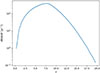 |
Fig. 1. Merging rate of seeded haloes (per unit redshift per year) for z ≤ 19.92. The time is shown in observer-frame units. The highest redshift corresponds to the highest available snapshot from the CAM25 model; only mergers below this redshift are considered. |
Figure 2 shows the timescale τH → G for the set of haloes discussed above and illustrated in Figure 1. It exhibits the expected trend (see, e.g. Somerville & Davé 2015), with mergers involving haloes with lower mass ratios taking much longer than the Hubble time to complete. Conversely, haloes with mass ratios closer to one can complete the galaxy merger within a Hubble time. Although most of these haloes have lower mass, a few heavier haloes with near-equal masses merge relatively quickly. The dispersion in the timescale is mainly due to the sampling of orbital eccentricities as mentioned above (CAM25).
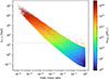 |
Fig. 2. Timescale from halo merger to galaxy merger, τH → G, as a function of the halo mass ratio. The colour of each point indicates the mass of the primary halo. The dashed grey line shows the Hubble time. |
τmerge – Once the galaxies have merged, we assume that the two BHs are at a separation equal to the radius of the remnant galaxy, which is on the order of a few kiloparsecs. Calculating the remaining time taken by the binary to merge is highly uncertain. This process involves modelling the internal dynamics of a galaxy and the interactions of stellar objects with the BHs. At separation of a few kiloparsecs, DF is sufficient to bring the BHs towards the galactic centre. Subsequently, the shrinking occurs primarily through three-body interactions with stars, which transfer angular momentum away from the binaries to the surrounding stellar population (‘stellar hardening’; e.g. Quinlan 1996; Sesana et al. 2006; Kelley et al. 2017; Barber et al. 2024). It is possible that the binaries do not undergo sufficient interactions to shrink further within Hubble timescales. This prevents the BHs from reaching the separations at which GWs dominate the orbit decay. This issue is known as the final parsec problem (e.g. Milosavljević & Merritt 2001; Merritt & Milosavljević 2005). However, various mechanisms have been proposed to address this problem, including the triaxiality of the galactic bulge or systems with multiple MBHs, among others (e.g. Yu 2002; Khan et al. 2011; Holley-Bockelmann & Khan 2015; Sesana & Khan 2015; Bonetti et al. 2016). Hence, it is reasonable to assume that the problem is solved. Computing the hardening timescale requires precise modelling of galaxy properties, which is beyond the scope of this work. For simplicity, we neglected both the hardening and the GW-dominated orbital decay timescales and considered only the DF timescale for τmerge, since it is the most significant contributor to the delay (e.g. see Fig. 11 in Langen et al. 2025).
To calculate the DF timescale, we employed the standard Chandrasekhar prescription (Chandrasekhar 1943; Binney & Tremaine 2008):
![Mathematical equation: $$ \begin{aligned} T_{\mathrm{dyn} } = 19 \left(\frac{r_0}{5\,\mathrm{kpc} }\right)^2\left(\frac{\sigma }{200 \mathrm{\ km} / \mathrm{s} }\right)\left(\frac{10^8 \mathrm{M} _{\odot }}{\mathrm{M} _{\mathrm{BH,s} }}\right) \frac{1}{\Lambda }[\mathrm{Gyr} ]. \end{aligned} $$](/articles/aa/full_html/2026/02/aa56833-25/aa56833-25-eq9.gif) (9)
(9)
Here, r0 is the initial separation of the BHs (which we set to the radius of the remnant galaxy), σ is the velocity dispersion of the remnant galaxy, and MBH, s is the mass of the secondary BH. The Coulomb logarithm, Λ, is given by Λ = ln(1 + M★/MBH, s), where M★ is the stellar mass of the remnant galaxy. To estimate the velocity dispersion, we used the scaling relation based on observations (Graham & Scott 2013; McConnell & Ma 2013; Kormendy & Ho 2013):
 (10)
(10)
We used only the mean value of the relation since the errors are small.
The Chandrasekhar formula (Equation (9)) assumes that the infalling BH from the secondary galaxy is completely stripped of its surrounding stellar component. However, many simulations show that stripping depends on galaxy morphology, orbital eccentricity, mass ratio, incidence angle, and more (see, e.g. Chang et al. 2013; Varisco et al. 2024). This implies that the primary galaxy does not interact with a point-like source, the BH, spiralling inward, but rather with an extended mass distribution consisting of the stellar component of the secondary galaxy, including the BH. Because the DF timescale is approximately inversely proportional to the infalling mass and carries the largest uncertainty1, the additional matter surrounding the secondary BH results in a reduced DF timescale. This implies that the timescale calculated from Equation 9 can be regarded as an upper limit. Since accurately modelling the stripping of the secondary galaxy is beyond the scope of this work, we modified Equation (9) to provide a simple lower-limit estimate of the timescale by assuming that the entire stellar mass of the secondary galaxy surrounds the infalling BH for the whole DF phase, such that
![Mathematical equation: $$ \begin{aligned} T_{\mathrm{dyn} }^\mathrm{ll} = 19 \left(\frac{r_{0,\mathrm{p} }}{5\mathrm{\ kpc} }\right)^2\left(\frac{\sigma }{200\mathrm{\ km} / \mathrm{s} }\right)\left(\frac{10^8 \mathrm{M} _{\odot }}{\mathrm{M} _{\star ,\mathrm{s} }}\right) \frac{1}{\Lambda ^\mathrm{ll} }[\mathrm{Gyr} ], \end{aligned} $$](/articles/aa/full_html/2026/02/aa56833-25/aa56833-25-eq11.gif) (11)
(11)
where the superscript ‘ll’ denotes the ‘lower limit’, subscripts ‘p’ and ‘s’ denote the properties of the primary and secondary galaxies, respectively, and Λll = ln(1 + M★, p/M★, s).
Another assumption of the Chandrasekhar formula is that the mass of the infalling object must be much larger than the mass of the field stars. Considering a typical initial stellar mass function (IMF) such as the standard four-part power law (Kroupa 2001, 2002; Weidner & Kroupa 2004), as well as the composite galactic-field IMF obtained by summing over all stellar clusters within a galaxy (Kroupa & Weidner 2003), most stars are less massive than 10 M⊙. Quantitatively, if we consider the galactic-field IMF from Kroupa & Weidner (2003) (see Fig. 1 therein) with stellar masses ranging from 0.01 M⊙ to 150 M⊙, then more than 99.92% of the stars are less massive than 10 M⊙ within a typical galaxy. This implies that the DF timescales calculated here would be valid for almost all inspiralling BHs more massive than ∼10 M⊙. Furthermore, this work focussed solely on estimating the merger rate for BHs in the intermediate and supermassive range that could be detected by LGWA and LISA. Based on these considerations, we restricted our analysis to BHs with masses above 10 M⊙.
As evident from the above equations, computing the DF requires knowledge of several galaxy properties, including the mass and radius, as well as the masses of the BHs. We used the CAM25 model to compute these quantities. In the next section, we describe how we used the model outputs to calculate these properties.
3.3. Scaling relations
As mentioned in Section 3.1, the CAM25 model provides baryonic properties, including the BH mass MBH, galaxy stellar mass m★, and the radius rg at discrete redshift snapshots. Figure 3 shows their scatter plots with respect to the halo mass at z = 0. The merger history of PINOCCHIO, however, has continuous time sampling and provides the exact redshift of each halo merger. As a DM-only code, the output also consists of the exact halo mass at the merging redshift. This motivated us to derive scaling relations between baryonic properties and the DM halo mass. These relations allowed us to use the halo mass at the exact merging redshift to calculate all the required properties used to evaluate the delays. In the following, we describe the method used to create these scaling relations.
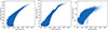 |
Fig. 3. Black hole (BH) mass, galaxy mass, and galaxy radius as a function of halo mass, derived from the CAM25 model with ALS seeding at z = 0. |
From each available CAM25 output at redshift zi, we divided the entire halo mass range into small bins [m1, m2] and created probability density functions (PDFs) f(Θ|zi, m1, m2) for each property Θ ∈ {MBH, m★, rg} across all the halo mass bins. This allowed us to construct a framework in which all baryonic properties of interest depend only on the redshift and the halo mass. To construct these PDFs, we generated histograms of the quantities Θ within small halo mass bins2 and used the scipy.stats library to convert them to PDFs.
To illustrate how we used these PDFs, consider the evaluation of a baryonic property Θ for a halo with mass mhalo, at redshift z. To calculate these properties, we used the PDFs of that property constructed above at the redshifts z1 and z2, where the CAM25 outputs were available, such that z ∈ [z1, z2], for the same halo mass bin, [m1, m2], where mhalo ∈ [m1, m2]. The corresponding PDFs at these redshifts are fi(Θ) = f(Θ|zi, m1, m2), with i = 1 or 2. We then linearly interpolated the PDFs in redshift space to compute the exact PDF at the required redshift z as follows:
 (12)
(12)
The redshift intervals of the CAM25 outputs are sufficiently small that the linear interpolation preserves the evolution of the baryonic properties. Once we calculated this distribution, f′, we computed the required PDF by normalising it as
 (13)
(13)
where the integral in the denominator is performed over the minimum and maximum values of Θ allowed by the model. This method allowed us to evaluate the baryonic properties at the exact merger redshifts using the DM halo mass provided by the merger history of PINOCCHIO.
3.4. Calculated delays
Using all the relations mentioned above, we finally calculated the properties required to evaluate the DF timescale for all merging galaxies and BHs. In the subsequent analysis, we considered only galaxies that either reach a stellar mass of 105 M⊙ by z = 0 or merge into a larger galaxy that reaches this mass by z = 0. This approach avoided imposing a fixed galaxy mass cut across all redshifts, which would be inappropriate given that galaxies at higher redshifts are less massive. The galaxy mass condition, together with a BH mass threshold of 10 M⊙ and a formation redshift cutoff of z = 8, are the only selection cuts used to define the merging population.
After applying the scaling relations and applying all the aforementioned cuts, we obtained the population of BH pairs shown in Figure 4, for which we calculated the DF timescales for the inspiral. These pairs form after adding the τH → G time delay (Figure 2) to the halo merger redshifts. Although Figure 2 shows that only haloes with high mass ratios merge, Figure 4 demonstrates that BH pairs spanning mass ratios of more than six orders of magnitude form within the age of the Universe. This behaviour arises from the combined growth of BHs and galaxies in the CAM25 model, which results in a larger variance in the dependence of these masses at lower halo masses. Most of these haloes subsequently merge within a Hubble time.
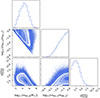 |
Fig. 4. Corner plot showing the distribution of the population of BH pairs formed after the galaxy merger. The plot shows the primary mass mBH, p, the secondary mass mBH, s divided by the primary BH mass mBH, s/mBH, p, and the redshift of the galaxy merger zmergegalaxy. The contours show the density of the points. Individual points outside the contours are also shown to visualize the extent of the distributions. |
As discussed in Section 3.2, after the galaxy merger, BHs are assumed to have a separation equal to the radius of the remnant galaxy, r0, in the upper-limit case (Equation (9)), while in the lower-limit case the separation is assumed to be equal to the radius of the primary galaxy, r0, p. Figure 5 shows a histogram of the separations for both cases. The distributions are quite similar, with most pairs having separations of the order of one kiloparsec. The difference is primarily due to a small excess of BHs at smaller separations in the r0, p case. This occurs because we used the mass of the primary halo to calculate the radius of the primary galaxy, which is smaller than the mass of the remnant halo used to calculate the radius of the remnant galaxy (see Section 3.3). Because of the small differences in their respective halo masses, the resulting radii are similar.
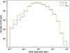 |
Fig. 5. Histogram of the initial BH separations used to compute the DF timescale. The separation r0 corresponds to the upper limit of the timescale (Equation (9)), while r0, p corresponds to the lower limit (Equation (11)). |
Next, we calculated both the upper and lower limits of the DF timescale using Equations (9) and (11), and present the results in Figure 6. The high BH mass ratio pairs show a stronger tendency to merge within a Hubble time, with a smaller scatter in the upper-limit case. This behaviour can be explained by considering Equation (9), which is used to evaluate the timescale. Ignoring the dependence on σ and Λ based on arguments presented in section 3.2, then Tdyn ∝ r02/MBH, s. Since more massive galaxies, especially those with larger haloes (see Figure 3), tend to have larger central BHs and radii, the radius dependence can be approximated by the primary BH mass, implying that Tdyn ∝ MBH, p2/MBH, s = (MBH, p/BH mass ratio). This approximation indicates that the timescale is longer for pairs with high primary BH masses and low mass ratios, whereas it is shorter for pairs with lower primary masses and higher mass ratios. We note that these approximations are more valid at higher halo masses because there is a greater spread in the baryonic properties at lower halo masses. This weakens the correlations and results in the spread in timescales, as seen in Figure 6. In the lower-limit case, the dependence on the mass ratio is weaker because we used the mass of the secondary galaxy, rather than the secondary BH, to evaluate the delay. This results in a slightly weaker dependence on the BH mass ratio, since a correlation between BH and galaxy mass persists, albeit weaker at these halo masses.
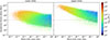 |
Fig. 6. Lower and upper limits of DF delays, in Myr, computed using Equations (11) and (9), respectively. The colour indicates the mass of the primary BH. The dashed horizontal line shows the age of the Universe. |
As a result of these trends, less than 2% of binaries have DF delays shorter than the Hubble time in the upper-limit case, while approximately 40% binaries do so in the lower-limit case. This behaviour is illustrated by the histogram of the timescales shown in Figure 7. Furthermore, in both cases, ∼60% of the binaries have total masses in the IMBH range, and ∼30% lie in the SMBH range. In the next section, we discuss the merger rates for these BH pairs.
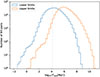 |
Fig. 7. Histogram of the DF delays for all pairs of BHs. The dashed line marks the age of the Universe. The lower and upper limits corresponds to the rates calculated using Equations (11) and (9), respectively. |
4. Results
4.1. Merging population
After applying the DF delays and assuming that the BHs merge shortly thereafter (see Sect. 3.2), we generated a population of merging BHs for both the lower- and upper-limit cases of the DF timescale. Figure 8 shows the merging BH pairs together with their corresponding merger redshifts. There is a significant difference in the number of BH pairs merging in the two cases, consistent with the discussion in Section 3.4.
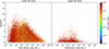 |
Fig. 8. Merging redshifts of all BH pairs as a function of the total binary mass for both the limits of DF timescale. The colour bar indicates the binary mass ratios. |
The median merger redshift in the lower-limit case is 1.18, while it decreases to 0.45 in the upper-limit case. This indicates that most mergers occur at low redshifts. Only a few binaries merge above z = 10 in the lower-limit case, whereas none do so in the upper-limit case. Although we considered all halo mergers below z ≈ 20, the actual merger rate at such high redshifts is quite low. The time span from z = 20 to z = 10 is only about 300 Myr, which is comparable to the minimum values of the additional delays that we applied, thereby limiting the number of mergers that can occur at high redshift.
Most merging pairs have mass ratios greater than 0.01: over 90% of the total merging population in the lower-limit case and more than 98% in the upper-limit case. For the mass range of MBHs considered, 87% of binaries with a total mass in the IMBH regime have mass ratios above 0.01 in the lower-limit case, increasing to more than 98% for the upper-limit case. A similar trend holds for the SMBH regime, with more than 87% of binaries mergers having a mass ratio above 0.01 in the lower-limit case and more than 95% in the upper-limit case. These results imply that most mergers are major, with only a very small percentage corresponding to intermediate or extreme mass-ratio inspirals and mergers.
To calculate the detectability of these mergers by GW detectors, we assigned random position in the sky to each source and computed the S/N using the GWFish3 library (Dupletsa et al. 2023). We calculated S/Ns using the IMRPhenomD waveform approximant (Husa et al. 2016; Khan et al. 2016) from the LALSimulation (LIGO Scientific Collaboration 2018), assuming observation durations of ten years for LGWA and four years for LISA. Figure 9 shows the S/Ns of events detectable by LISA and LGWA for both the lower- and upper-limit DF timescales. For simplicity, we assumed that all BHs are spinless and do not receive a kick after the merger, which could potentially eject them from the galaxy centre (Campanelli et al. 2007; Blecha & Loeb 2008; Tanaka & Haiman 2009). We assumed that all events with S/N > 8 were detectable. As expected from the design sensitivities of the detectors, LGWA can detect more binaries with an intermediate-mass range and higher S/Ns compared to LISA.
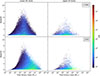 |
Fig. 9. Signal-to-noise ratio (S/N) of all merging events as observed by LGWA (top row) and LISA (bottom row). Only events with S/N > 8 are shown. |
4.2. Merger rate
To track the evolution of the merger rate, we calculated the quantity dN/dtdz, which gives the number of mergers per unit redshift and year using the relation
 (14)
(14)
where dn/dz is the differential number of BH mergers per unit comoving volume per redshift bin, and dc(z) is the comoving distance at redshift z. Time is expressed in observer-frame units. Given the statistical nature of our model, we performed our entire analysis twenty times to calculate an average rate with dispersion. Performing the analysis multiple times builds robust statistics, particularly at higher redshifts where merger numbers are low. The merger rates corresponding to the lower DF limit represents the optimistic case, while those for the upper DF timescale limits represent the pessimistic case. In the next two subsections, we present the rates for mergers of all BHs and for specific mass ranges of interest.
4.2.1. All masses
In Figure 10, we present the rates for all BH masses. The left panel shows the rates for all the mergers without convolving them with the sensitivity curves of the two detectors. The merger rate curves follow the shape of the halo merger rate (Figure 1). However, due to the inclusion of delays, the merger peak shifts to a lower redshift. In the optimistic case, the peak occurs around z ∼ 2, while in the pessimistic case, it shifts to z ∼ 1. At high redshift, mergers start occurring at z ∼ 14 in the optimistic case, although the dispersion is large due to both the low number of mergers and the dispersion in merging time delays. In the pessimistic case, mergers only occur only below z ∼ 8. Although the difference between the two cases is large at higher redshifts, it decreases at lower redshifts, reaching only about an order of magnitude by z = 0.
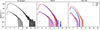 |
Fig. 10. Number of mergers per unit redshift per year at different redshifts, as detected by the two detectors for two cuts on the S/Ns. The time is reported in the observer frame. The lines show the average rates over 20 realisations, while the shaded region indicates the 1σ deviation from the mean. The solid lines and darker shaded region corresponds to the rates calculated using the lower limits on the DF, while the dashed lines and lighter shaded region corresponds to the upper limits. The left panel shows the rate for all mergers in our model, while the middle and right panels shows the rates for mergers detected by LGWA (blue) and LISA (red) with minimum S/Ns of 8 and 100, respectively. |
In the remaining panels of the figure, we present the rates after convolving with the sensitivity curves of LISA and LGWA. For all sources with S/N > 8, the rates for both detectors are similar. In the pessimistic case, the rates are also similar to the rate for all mergers shown in the left panel. This result implies that most of the merging population constructed by considering the upper limits of the DF timescales will be detectable by both detectors. In the optimistic case, the rates are slightly lower than those for all mergers, especially at higher redshifts. The LGWA detector is able to detect mergers at slightly higher redshifts, around ∼11, compared to LISA. However, the overall distribution of rates for both detectors is similar. A difference emerges for sources with S/N > 100 in the optimistic case. The LISA detector is able to detect more mergers up to z ∼ 7, while LGWA does not detect mergers with such high S/N at redshifts beyond z ∼ 5. The rates in the pessimistic case remain similar.
4.2.2. Mass ranges
Figure 11 shows the evolution of merger rates for three total binary mass intervals – [103, 105] M⊙, [105, 107] M⊙, and [107, 108] M⊙ – each evaluated with two different S/N cuts. The first column also shows the rates for all merging binaries, without any S/N cut. For the intermediate-mass range binaries, the merger rates detected by both detectors with S/N > 8 are similar for both the optimistic and pessimistic cases. The LGWA detector has a slightly higher rate and detects mergers at slightly higher redshifts in the optimistic case, reaching up to z ∼ 11. However, the difference becomes much more pronounced for events detected with S/N greater than 100 in both cases. This behaviour is expected because LGWA has a higher sensitivity to these mass ranges than LISA.
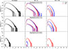 |
Fig. 11. Merger rate evolution in the observer frame for all binaries within mass ranges [103, 105] M⊙, [105, 107] M⊙, and [107, 108] M⊙. The first column shows the rate for all the mergers, while the remaining columns show the rate for events with S/N > 8 and 100 as seen by the detectors. The colour scheme is the same as in Figure 10. |
For more massive BHs (105 to 107 M⊙), the roles reverse and LISA shows higher detection rates. Again, the difference in rates is small for detections with S/N > 8 in both cases. At a higher S/N cut, LISA’s detection rates for these binary BHs are significantly higher and reach redshifts beyond those of LGWA, especially in the optimistic case. In the pessimistic case, the difference persists, although less pronounced. This implies that the similar rates at lower S/N cuts arise because LISA detects a similar number of mergers, but with much higher S/N. Finally, for the most massive BHs (107 to 108 M⊙), LISA detects significantly more events in the optimistic case and reaches redshifts higher than those of LGWA. In the pessimistic case, the rates are similar for the lower S/N cut. The evolution of the rate in the optimistic case for LISA is similar for both the S/N cuts, resembling that of all mergers in this mass range. This implies that LISA detects most of these mergers with a high S/N.
4.2.3. Total detections per year
To calculate the total number of detections per year, we integrated dN/dtdz obtained from Equation (14) over the entire redshift range. Table 1 reports the total number of mergers per year in the observer frame after the integration. These numbers represent the averages of our twenty realisations of the merging population, as shown in Figures 10 and 11. For all BH binaries, the pessimistic case predicts an average of only 0.61 mergers per year, while in the optimistic case this number rises to nearly 50 per year. Of these, both LGWA and LISA would detect about 0.5 mergers per year in the pessimistic scenario, increasing to more than 26 detections per year in the optimistic scenario. Despite the significant difference in the number of possible detections between the two cases, given the expected lifetime of LGWA (ten years) and LISA (four years), even the pessimistic case results in some detections with S/N > 8. This implies a high probability of several detections within the lifetime of these detectors.
Number of mergers detected per year by the two detectors for different S/N cuts.
For binaries with total mass in the intermediate range, detection numbers are low. However, over their expected lifetimes, LGWA should detect at least a few mergers, and LISA may observe at least one in the pessimistic case. In the optimistic scenario, both detectors could observe many mergers. Furthermore, some sources with higher S/N should also be detectable. As expected, LGWA has detection rates higher than LISA for these binary masses. For the binaries in the supermassive regime, the detectability trend reverses, and LISA has the potential to detect more mergers than LGWA. For binaries in the range 105 M⊙ to 107 M⊙, the rate difference in the pessimistic case is small, although the difference in the lifetime of these detectors may play a major role in the total detection numbers. In the optimistic case, there are many more detections, with at least seven per year for LGWA and more than 11 per year for LISA. As in the case for LGWA at lower binary masses, LISA will also be able to detect higher mass binaries with a higher S/N. Finally, for the most massive BHs, the rates are low, as expected, since these detectors are not expected to detect their mergers within their lifetimes.
The similar detection rates for sources with S/N > 8 in both detectors suggest a strong potential for synergy. If both detectors are active at the same time, the lower-frequency sensitivity of LISA allows a potential binary to be observed at an inspiral stage, which then merges at frequencies sensitive to LGWA. This is especially true for BH binaries with masses in the range ∼103 M⊙ to 104 M⊙ (Colpi et al. 2024). Given the high detection rates for these masses, this synergy offers a valuable opportunity to study a still-elusive BH population and place strong constraints on the BH mass function in this range.
4.2.4. Comparison with other models
As mentioned briefly in the introduction, the predicted merger rate from different models depends heavily on the model assumptions and the considered physical processes, particularly the seed BH mass and merger delays. Furthermore, the rates also depend on the simulation resolution (both spatial and mass), the simulation volume, the simulated redshift range, and other factors. Due to all these differences among models, a faithful comparison is not entirely feasible. However, estimates from different models can help us to understand the range of detections expected from LISA and LGWA.
To date, most population studies have focussed on the observational sensitivity of LISA. For instance, in the semi-analytical formulation of Ricarte & Natarajan (2018) with their light-seed implementation, they predict that LISA will detect around ∼40 to ∼245 mergers per year with S/N > 5 in their pessimistic and optimistic models, respectively. These models are based on the merging probability of BHs after the merging of their parent haloes. For heavy seeds, the rates drop to ∼5 to ∼48 per year for the two cases.
Conversely, Volonteri et al. (2020) present a lower merger rate of MBHs from the high-resolution simulation NEWHORIZON (Dubois et al. 2021). Depending on the adopted delays, the rate varies from ∼1 to ∼10 MBH mergers per year. These are total merger rates from the simulation and are not convolved with the sensitivity curve of LISA. In the work of Barausse et al. (2020), which is based on the SAM first presented in Barausse (2012), the detection rate is ≳2 mergers per year with LISA, irrespective of the BH seeding scheme. However, the rates depend significantly on the delays and on the impact of supernova feedback on MBH growth.
Kritos et al. (2025) implemented the formation and evolution of MBHs in the centre of nuclear star clusters using the galaxy merger trees from NEWHORIZON and applying the NUCE SAM (Kritos et al. 2024). They report a merger rate of ≃5.3 mergers per year up to z = 5. Compared to all these studies and the broader literature, our model predictions are consistent. Measurements of the rate from LISA will help to constrain these models, allowing us to better understand the physical processes driving MBH mergers.
5. Summary and Conclusions
We investigated the formation and merger rate of IMBH and SMBH binaries, focussing on their detectability by the upcoming gravitational-wave detectors LGWA and LISA. We generated the binary population using a light-seed scenario consistent with Pop III seeding, applying the CAM25 model to merger trees from a PINOCCHIO simulation with a 40 Mpc/h box. The CAM25 model was then used to estimate the baryonic properties of the host galaxies and the growth of the BHs through mergers and accretion. From the halo-merger redshifts provided by the simulation, we calculated the BH merger redshifts by adding two time delays: the halo-to-galaxy merger and the galaxy-to-BH merger. To calculate the first delay, we use the prescription in CAM25. For the second delay, we considered only the DF timescale.
To estimate the second delay, we applied the Chandrasekhar prescription to compute the time taken by the secondary BH to sink towards the centre. We considered two limiting cases for this delay: one in which the secondary BH is completely stripped of all surrounding stellar material for the entire plunge and the other in which the stellar material of the secondary galaxy remains intact for the entire timescale. The former provides an upper limit on the timescale, while the latter provides a lower limit.
After calculating the DF timescales for each pair of BHs, we constructed the populations of merging BHs. We then randomly distributed all events on the sky and evaluated their S/Ns as observed by the LGWA and LISA detectors. In the following, we summarise our main findings for the detected population, along with the estimated timescales:
-
In the lower limit scenario for the DF timescale, the number of mergers completing within a Hubble time is significantly larger than in the upper limit case. Of the entire population of BH pairs, only 2% have delays less than the Hubble time in the upper limits case, whereas nearly 40% have a shorter delay in the lower limits case. The difference mainly comes from using the entire stellar mass of the secondary galaxy in evaluating the delay instead of just the BH mass. This reduces the delay by a few orders of magnitude and highlights the importance of accurately modelling galaxy stripping to estimate BH merger timescales.
-
The larger number of mergers completing within the age of the Universe in the lower-limit case defines our optimistic merger-rate scenario, while the upper-limit case represents a pessimistic scenario. In both cases, the majority of mergers are major, with mass ratios typically exceeding 0.01.
-
The redshift distribution of mergers strongly depends on the assumed timescale: in the optimistic scenario, BH mergers can occur as early as z ∼ 14, while in the pessimistic case, they mostly occur at z < 8. The difference in rates among the two cases is larger at higher redshifts, while it decreases at lower redshifts, reaching only about an order-of-magnitude difference at z = 0. Despite these differences, most detectable events occur at lower redshifts (z < 3).
-
We evaluated the GW signal strength of each merger and assessed its detectability with LISA and LGWA. Both LGWA and LISA can detect approximately 25 mergers per year in the optimistic case, including all BH masses. However, this number reduces to around 0.5 per year in the pessimistic case.
-
For the expected 10-year lifetime of LGWA, our model predicts that it will detect a total of ∼260 mergers in the optimistic case, while only ∼5 in the pessimistic case. In contrast, LISA is expected to be active for four years, yielding a total of ∼105 and ∼2 merger detections in the optimistic and pessimistic cases, respectively.
-
For binaries with total mass in the intermediate range, the number of detections per year for LGWA ranges from ∼0.34 in the pessimistic case to ∼20 in the optimistic case. For LISA, the number of detected events is slightly lower, ranging from ∼0.3 to ∼15 in the two cases, respectively. For detections with higher S/N, LGWA has a higher detection rate, as expected. However, detections with S/N greater than 100 are rare, with only ∼1 per year for LISA and ∼2.7 for LGWA, both in the optimistic case.
-
For binaries in the range 105 M⊙ to 107 M⊙, the detection tendency reverses, and LISA detects more than ∼11 mergers per year in the optimistic case, compared to ∼7 for LGWA. For binaries detected with S/N > 100, LISA is still able to detect more than ∼6 mergers per year in the optimistic case, compared to fewer than one for LGWA. For the most massive binaries with Mbin > 107 M⊙, the rates are low, which is expected, since these BHs lie outside the design sensitivity of the detectors.
-
The merger rates obtained from our model for LISA are consistent with those reported above and with the literature, despite differences in the modelling and simulations.
Finally, we note that in our calculation of the DF timescale, we only considered the variation in the mass of the infalling object, which resulted in a difference of orders of magnitude. Given this large variance, we expect that other assumptions, particularly the assumption of initial separation as the radius of the remnant (or primary) galaxy, will not make a significant difference in the calculation of this timescale. We also note that in this work we only followed the formation of binaries through the galaxy merger channel. This implies that binaries formed through other channels are not included, such as IMBHs formed through runaway stellar mergers or the formation of intermediate- or extreme-mass-ratio inspirals. These binaries can also be detected by LGWA and LISA, which implies that the total detection rate of BH binaries could be even higher than the results presented here. Nevertheless, both detectors offer complementary sensitivity across different mass and redshift regimes. The combination of LISA and LGWA will be essential to probe the full BH mass spectrum, from the elusive intermediate-mass to the supermassive regimes, and from major mergers with high mass ratio to extreme-mass-ratio inspirals. Furthermore, because the merging redshifts and the number density of mergers depend on the formation and seeding mechanisms of BHs, the detections of their mergers will also help to constrain those mechanisms.
Acknowledgments
We thank the anonymous referee for the useful and constructive comments which improved the quality of the paper. We acknowledge a financial contribution from the Bando Ricerca Fondamentale INAF 2022 Large Grant, ‘Dual and binary supermassive black holes in the multi-messenger era: from galaxy mergers to gravitational waves’ and from the INAF Bando Ricerca Fondamentale INAF 2024 Large Grant, ‘The Quest for dual and binary massive black holes in the gravitational wave era’. We acknowledge financial support from the Italian Space Agency (ASI) under Grant No. 2025-29-HH.0. We also acknowledge the support of the computing centre of INAF-Osservatorio Astronomico di Trieste, under the coordination of the CHIPP project Bertocco et al. (2020), Taffoni et al. (2020). JS thanks David Izquierdo-Villalba, Elisa Bortolas, and Manuel Arca Sedda for helpful discussions on DF and the referee report. VC thanks the BlackHoleWeather ERC project and PI Prof. Gaspari for salary support. JCT acknowledges support from ERC Advanced Grant 788829 (MSTAR). The data underlying this article will be shared on reasonable request to the corresponding author.
References
- Abac, A. G., Abouelfettouh, I., Acernese, F., et al. 2025, ApJ, 993, L25 [Google Scholar]
- Abbott, B. P., Abbott, R., Abbott, T. D., et al. 2016, Phys. Rev. Lett., 116, 061102 [Google Scholar]
- Abel, T., Bryan, G. L., & Norman, M. L. 2002, Science, 295, 93 [CrossRef] [Google Scholar]
- Agazie, G., Alam, M. F., Anumarlapudi, A., et al. 2023a, ApJ, 951, L9 [CrossRef] [Google Scholar]
- Agazie, G., Anumarlapudi, A., Archibald, A. M., et al. 2023b, ApJ, 951, L8 [NASA ADS] [CrossRef] [Google Scholar]
- Ajith, P., Seoane, P. A., Arca Sedda, M., et al. 2025, JCAP, 2025, 108 [Google Scholar]
- Amaro-Seoane, P., Aoudia, S., Babak, S., et al. 2013, GW Notes, 6, 4 [Google Scholar]
- Amaro-Seoane, P., Andrews, J., Arca Sedda, M., et al. 2023, Living Rev. Rel., 26, 2 [Google Scholar]
- Antonini, F., Gieles, M., & Gualandris, A. 2019, MNRAS, 486, 5008 [NASA ADS] [CrossRef] [Google Scholar]
- Arca Sedda, M., Askar, A., & Giersz, M. 2018, MNRAS, 479, 4652 [NASA ADS] [CrossRef] [Google Scholar]
- Banik, N., Tan, J. C., & Monaco, P. 2019, MNRAS, 483, 3592 [NASA ADS] [CrossRef] [Google Scholar]
- Barausse, E. 2012, MNRAS, 423, 2533 [NASA ADS] [CrossRef] [Google Scholar]
- Barausse, E., Dvorkin, I., Tremmel, M., Volonteri, M., & Bonetti, M. 2020, ApJ, 904, 16 [NASA ADS] [CrossRef] [Google Scholar]
- Barber, J., Chattopadhyay, D., & Antonini, F. 2024, MNRAS, 527, 7363 [Google Scholar]
- Berner, P., Refregier, A., Sgier, R., et al. 2022, JCAP, 2022, 002 [Google Scholar]
- Bertocco, S., Goz, D., Tornatore, L., et al. 2020, ASP Conf. Ser., 527, 303 [NASA ADS] [Google Scholar]
- Bhowmick, A. K., Blecha, L., Torrey, P., et al. 2022, MNRAS, 510, 177 [Google Scholar]
- Binney, J., & Tremaine, S. 2008, Galactic Dynamics, Second Edition (Princeton University Press) [Google Scholar]
- Birrer, S., Lilly, S., Amara, A., Paranjape, A., & Refregier, A. 2014, ApJ, 793, 12 [NASA ADS] [CrossRef] [Google Scholar]
- Blecha, L., & Loeb, A. 2008, MNRAS, 390, 1311 [NASA ADS] [Google Scholar]
- Boekholt, T. C. N., Schleicher, D. R. G., Fellhauer, M., et al. 2018, MNRAS, 476, 366 [Google Scholar]
- Bonetti, M., Haardt, F., Sesana, A., & Barausse, E. 2016, MNRAS, 461, 4419 [NASA ADS] [CrossRef] [Google Scholar]
- Boylan-Kolchin, M., Ma, C.-P., & Quataert, E. 2008, MNRAS, 383, 93 [Google Scholar]
- Bromm, V., & Loeb, A. 2003, ApJ, 596, 34 [Google Scholar]
- Bromm, V., Yoshida, N., & Hernquist, L. 2003, ApJ, 596, L135 [Google Scholar]
- Cammelli, V., Monaco, P., Tan, J. C., et al. 2025, MNRAS, 536, 851 [Google Scholar]
- Campanelli, M., Lousto, C., Zlochower, Y., & Merritt, D. 2007, ApJ, 659, L5 [NASA ADS] [CrossRef] [Google Scholar]
- Carr, B. J. 2005, ArXiv e-prints [arXiv:astro-ph/0511743] [Google Scholar]
- Chandrasekhar, S. 1943, ApJ, 97, 255 [Google Scholar]
- Chang, J., Macciò, A. V., & Kang, X. 2013, MNRAS, 431, 3533 [NASA ADS] [CrossRef] [Google Scholar]
- Chon, S., & Omukai, K. 2020, MNRAS, 494, 2851 [Google Scholar]
- Chon, S., Hirano, S., Hosokawa, T., & Yoshida, N. 2016, ApJ, 832, 134 [NASA ADS] [CrossRef] [Google Scholar]
- Colpi, M., Danzmann, K., Hewitson, M., et al. 2024, ArXiv e-prints [arXiv:2402.07571] [Google Scholar]
- Dayal, P. 2024, A&A, 690, A182 [NASA ADS] [CrossRef] [EDP Sciences] [Google Scholar]
- De Lucia, G., Fontanot, F., Xie, L., & Hirschmann, M. 2024, A&A, 687, A68 [NASA ADS] [CrossRef] [EDP Sciences] [Google Scholar]
- Di Matteo, T., Colberg, J., Springel, V., Hernquist, L., & Sijacki, D. 2008, ApJ, 676, 33 [NASA ADS] [CrossRef] [Google Scholar]
- Dubois, Y., Beckmann, R., Bournaud, F., et al. 2021, A&A, 651, A109 [NASA ADS] [CrossRef] [EDP Sciences] [Google Scholar]
- Dupletsa, U., Harms, J., Banerjee, B., et al. 2023, Astron. Comput., 42, 100671 [NASA ADS] [CrossRef] [Google Scholar]
- Ebisuzaki, T. 2003, IAU Symp., 208, 157 [Google Scholar]
- EPTA Collaboration (Antoniadis, J., et al.) 2023, A&A, 678, A48 [Google Scholar]
- Euclid Collaboration (Monaco, P., et al.) 2025, A&A, 704, A306 [Google Scholar]
- Event Horizon Telescope Collaboration (Akiyama, K., et al.) 2019, ApJ, 875, L1 [Google Scholar]
- Event Horizon Telescope Collaboration (Akiyama, K., et al.) 2022, ApJ, 930, L12 [NASA ADS] [CrossRef] [Google Scholar]
- Feng, W.-X., Yu, H.-B., & Zhong, Y.-M. 2021, ApJ, 914, L26 [NASA ADS] [CrossRef] [Google Scholar]
- Ferrarese, L., & Ford, H. 2005, Space Sci. Rev., 116, 523 [Google Scholar]
- Fontanot, F., De Lucia, G., Hirschmann, M., et al. 2020, MNRAS, 496, 3943 [CrossRef] [Google Scholar]
- Giersz, M., Leigh, N., Hypki, A., Lützgendorf, N., & Askar, A. 2015, MNRAS, 454, 3150 [Google Scholar]
- Graham, A. W., & Scott, N. 2013, ApJ, 764, 151 [Google Scholar]
- Greene, J. E., Strader, J., & Ho, L. C. 2020, ARA&A, 58, 257 [Google Scholar]
- Greif, T. H., & Bromm, V. 2006, MNRAS, 373, 128 [NASA ADS] [CrossRef] [Google Scholar]
- Guo, Q., White, S., Boylan-Kolchin, M., et al. 2011, MNRAS, 413, 101 [Google Scholar]
- Habouzit, M., Volonteri, M., Latif, M., Dubois, Y., & Peirani, S. 2016, MNRAS, 463, 529 [NASA ADS] [CrossRef] [Google Scholar]
- Haemmerlé, L., Mayer, L., Klessen, R. S., et al. 2020, Space Sci. Rev., 216, 48 [Google Scholar]
- Harikane, Y., Zhang, Y., Nakajima, K., et al. 2023, ApJ, 959, 39 [NASA ADS] [CrossRef] [Google Scholar]
- Harms, J., Ambrosino, F., Angelini, L., et al. 2021, ApJ, 910, 1 [NASA ADS] [CrossRef] [Google Scholar]
- Hawking, S. 1971, MNRAS, 152, 75 [Google Scholar]
- Hirschmann, M., De Lucia, G., & Fontanot, F. 2016, MNRAS, 461, 1760 [Google Scholar]
- Holley-Bockelmann, K., & Khan, F. M. 2015, ApJ, 810, 139 [Google Scholar]
- Husa, S., Khan, S., Hannam, M., et al. 2016, Phys. Rev. D, 93, 044006 [NASA ADS] [CrossRef] [Google Scholar]
- Inayoshi, K., Visbal, E., & Haiman, Z. 2020, ARA&A, 58, 27 [NASA ADS] [CrossRef] [Google Scholar]
- Izquierdo-Villalba, D., Bonoli, S., Dotti, M., et al. 2020, MNRAS, 495, 4681 [NASA ADS] [CrossRef] [Google Scholar]
- Izquierdo-Villalba, D., Sesana, A., Bonoli, S., & Colpi, M. 2022, MNRAS, 509, 3488 [Google Scholar]
- Jaacks, J., Finkelstein, S. L., & Bromm, V. 2019, MNRAS, 488, 2202 [NASA ADS] [CrossRef] [Google Scholar]
- Jani, K., Abernathy, M., Berti, E., et al. 2025, ArXiv e-prints [arXiv:2508.11631] [Google Scholar]
- Johnson, J. L., Dalla Vecchia, C., & Khochfar, S. 2013, MNRAS, 428, 1857 [NASA ADS] [CrossRef] [Google Scholar]
- Kawamura, S., Ando, M., Seto, N., et al. 2021, Prog. Theor. Exp. Phys., 2021, 05A105 [CrossRef] [Google Scholar]
- Kelley, L. Z., Blecha, L., & Hernquist, L. 2017, MNRAS, 464, 3131 [NASA ADS] [CrossRef] [Google Scholar]
- Khan, F. M., Just, A., & Merritt, D. 2011, ApJ, 732, 89 [Google Scholar]
- Khan, S., Husa, S., Hannam, M., et al. 2016, Phys. Rev. D, 93, 044007 [Google Scholar]
- Kormendy, J., & Ho, L. C. 2013, ARA&A, 51, 511 [Google Scholar]
- Kritos, K., Berti, E., & Silk, J. 2024, MNRAS, 531, 133 [Google Scholar]
- Kritos, K., Beckmann, R. S., Silk, J., et al. 2025, ApJ, 991, 58 [Google Scholar]
- Kroupa, P. 2001, MNRAS, 322, 231 [NASA ADS] [CrossRef] [Google Scholar]
- Kroupa, P. 2002, Science, 295, 82 [Google Scholar]
- Kroupa, P., & Weidner, C. 2003, ApJ, 598, 1076 [NASA ADS] [CrossRef] [Google Scholar]
- Langen, V., Tamanini, N., Marsat, S., & Bortolas, E. 2025, MNRAS, 536, 3366 [Google Scholar]
- Latif, M. A., Schleicher, D. R. G., Schmidt, W., & Niemeyer, J. 2013, MNRAS, 433, 1607 [NASA ADS] [CrossRef] [Google Scholar]
- LIGO Scientific Collaboration (Aasi, J., et al.) 2015, Classical Quantum Gravity, 32, 074001 [NASA ADS] [CrossRef] [Google Scholar]
- LIGO Scientific Collaboration, Virgo Collaboration,& KAGRA Collaboration 2018, LVK Algorithm Library - LALSuite, Free software (GPL) [Google Scholar]
- LISA Consortium Waveform Working Group (Afshordi, N., et al.) 2025, Liv. Rev. Rel., 28, 9 [Google Scholar]
- Liu, B., & Bromm, V. 2020, MNRAS, 497, 2839 [NASA ADS] [CrossRef] [Google Scholar]
- Luo, J., Chen, L.-S., Duan, H.-Z., et al. 2016, Classical Quantum Gravity, 33, 035010 [NASA ADS] [CrossRef] [Google Scholar]
- Luo, J., Bai, S., Bai, Y., et al. 2025, Classical and Quantum Gravity, 42, 173001 [Google Scholar]
- Lupi, A., Trinca, A., Volonteri, M., Dotti, M., & Mazzucchelli, C. 2024, A&A, 689, A128 [NASA ADS] [CrossRef] [EDP Sciences] [Google Scholar]
- Lusso, E., Valiante, R., & Vito, F. 2023, in Handbook of X-ray and Gamma-ray Astrophysics, eds. C. Bambi, & A. Santangelo (Singapore: Springer Nature), 122 [Google Scholar]
- Madau, P., & Rees, M. J. 2001, ApJ, 551, L27 [Google Scholar]
- Maio, U., Borgani, S., Ciardi, B., & Petkova, M. 2019, PASA, 36 [Google Scholar]
- McConnell, N. J., & Ma, C.-P. 2013, ApJ, 764, 184 [Google Scholar]
- McKee, C. F., & Tan, J. C. 2008, ApJ, 681, 771 [NASA ADS] [CrossRef] [Google Scholar]
- Mebane, R. H., Mirocha, J., & Furlanetto, S. R. 2018, MNRAS, 479, 4544 [NASA ADS] [CrossRef] [Google Scholar]
- Merritt, D., & Milosavljević, M. 2005, Living Rev. Rel., 8, 8 [Google Scholar]
- Milosavljević, M., & Merritt, D. 2001, ApJ, 563, 34 [Google Scholar]
- Mo, H. J., & White, S. D. M. 2002, MNRAS, 336, 112 [Google Scholar]
- Mo, H. J., Mao, S., & White, S. D. M. 1998, MNRAS, 295, 319 [Google Scholar]
- Monaco, P., Theuns, T., & Taffoni, G. 2002, MNRAS, 331, 587 [Google Scholar]
- Moutarde, F., Alimi, J. M., Bouchet, F. R., Pellat, R., & Ramani, A. 1991, ApJ, 382, 377 [Google Scholar]
- Munari, E., Monaco, P., Sefusatti, E., et al. 2017, MNRAS, 465, 4658 [Google Scholar]
- Planck Collaboration VI. 2020, A&A, 641, A6 [NASA ADS] [CrossRef] [EDP Sciences] [Google Scholar]
- Portegies Zwart, S. F., Baumgardt, H., Hut, P., Makino, J., & McMillan, S. L. W. 2004, Nature, 428, 724 [Google Scholar]
- Quinlan, G. D. 1996, New Astron., 1, 35 [Google Scholar]
- Reardon, D. J., Zic, A., Shannon, R. M., et al. 2023, ApJ, 951, L6 [NASA ADS] [CrossRef] [Google Scholar]
- Ricarte, A., & Natarajan, P. 2018, MNRAS, 481, 3278 [NASA ADS] [CrossRef] [Google Scholar]
- Rizzuto, F. P., Naab, T., Rantala, A., et al. 2023, MNRAS, 521, 2930 [NASA ADS] [CrossRef] [Google Scholar]
- Sesana, A., & Khan, F. M. 2015, MNRAS, 454, L66 [Google Scholar]
- Sesana, A., Haardt, F., & Madau, P. 2006, ApJ, 651, 392 [Google Scholar]
- Shang, C., Bryan, G. L., & Haiman, Z. 2010, MNRAS, 402, 1249 [NASA ADS] [CrossRef] [Google Scholar]
- Sijacki, D., Springel, V., Di Matteo, T., & Hernquist, L. 2007, MNRAS, 380, 877 [NASA ADS] [CrossRef] [Google Scholar]
- Singh, J., Monaco, P., & Tan, J. C. 2023, MNRAS, 525, 969 [NASA ADS] [CrossRef] [Google Scholar]
- Somerville, R. S., & Davé, R. 2015, ARA&A, 53, 51 [Google Scholar]
- Spinoso, D., Bonoli, S., Valiante, R., Schneider, R., & Izquierdo-Villalba, D. 2023, MNRAS, 518, 4672 [Google Scholar]
- Taffoni, G., Becciani, U., Garilli, B., et al. 2020, ASP Conf. Ser., 527, 307 [NASA ADS] [Google Scholar]
- Tagawa, H., Haiman, Z., & Kocsis, B. 2020, ApJ, 892, 36 [Google Scholar]
- Tan, J. C., & McKee, C. F. 2004, ApJ, 603, 383 [CrossRef] [Google Scholar]
- Tan, J. C., Smith, B. D., & O’Shea, B. W. 2010, AIP Conf. Proc., 1294, 34 [Google Scholar]
- Tanaka, T., & Haiman, Z. 2009, ApJ, 696, 1798 [NASA ADS] [CrossRef] [Google Scholar]
- Trinca, A., Schneider, R., Valiante, R., et al. 2022, MNRAS, 511, 616 [NASA ADS] [CrossRef] [Google Scholar]
- Valiante, R., Schneider, R., Volonteri, M., & Omukai, K. 2016, MNRAS, 457, 3356 [NASA ADS] [CrossRef] [Google Scholar]
- Valiante, R., Colpi, M., Schneider, R., et al. 2021, MNRAS, 500, 4095 [Google Scholar]
- Varisco, L., Dotti, M., Bonetti, M., Bortolas, E., & Lupi, A. 2024, A&A, 689, A279 [NASA ADS] [CrossRef] [EDP Sciences] [Google Scholar]
- Vogelsberger, M., Genel, S., Springel, V., et al. 2014, MNRAS, 444, 1518 [Google Scholar]
- Volonteri, M. 2010, A&ARv, 18, 279 [Google Scholar]
- Volonteri, M., Natarajan, P., & Gültekin, K. 2011, ApJ, 737, 50 [NASA ADS] [CrossRef] [Google Scholar]
- Volonteri, M., Dubois, Y., Pichon, C., & Devriendt, J. 2016, MNRAS, 460, 2979 [Google Scholar]
- Volonteri, M., Pfister, H., Beckmann, R. S., et al. 2020, MNRAS, 498, 2219 [Google Scholar]
- Weidner, C., & Kroupa, P. 2004, MNRAS, 348, 187 [NASA ADS] [CrossRef] [Google Scholar]
- Whalen, D., O’Shea, B. W., Smidt, J., & Norman, M. L. 2008a, ApJ, 679, 925 [NASA ADS] [CrossRef] [Google Scholar]
- Whalen, D., van Veelen, B., O’Shea, B. W., & Norman, M. L. 2008b, ApJ, 682, 49 [Google Scholar]
- Wise, J. H., Turk, M. J., Norman, M. L., & Abel, T. 2012, ApJ, 745, 50 [NASA ADS] [CrossRef] [Google Scholar]
- Wise, J. H., Regan, J. A., O’Shea, B. W., et al. 2019, Nature, 566, 85 [NASA ADS] [CrossRef] [Google Scholar]
- Xie, L., De Lucia, G., Hirschmann, M., Fontanot, F., & Zoldan, A. 2017, MNRAS, 469, 968 [Google Scholar]
- Xu, H., Chen, S., Guo, Y., et al. 2023, Res. Astron. Astrophys., 23, 075024 [CrossRef] [Google Scholar]
- Yu, Q. 2002, MNRAS, 331, 935 [Google Scholar]
- Zentner, A. R., Berlind, A. A., Bullock, J. S., Kravtsov, A. V., & Wechsler, R. H. 2005, ApJ, 624, 505 [NASA ADS] [CrossRef] [Google Scholar]
- Zoldan, A., De Lucia, G., Xie, L., Fontanot, F., & Hirschmann, M. 2019, MNRAS, 487, 5649 [NASA ADS] [CrossRef] [Google Scholar]
σ weakly depends on MBH, p, and Λ is equivalent to 𝒪(1). The radius of the galaxy, which is calculated using a scaling relation based on the DM halo mass (see next section), does not change significantly if we use the mass of the primary DM halo or the sum of primary and secondary DM halo masses (see Figure 5).
The bins are small enough to preserve the correlation among properties.
All Tables
Number of mergers detected per year by the two detectors for different S/N cuts.
All Figures
|
Fig. 1. Merging rate of seeded haloes (per unit redshift per year) for z ≤ 19.92. The time is shown in observer-frame units. The highest redshift corresponds to the highest available snapshot from the CAM25 model; only mergers below this redshift are considered. |
| In the text | |
|
Fig. 2. Timescale from halo merger to galaxy merger, τH → G, as a function of the halo mass ratio. The colour of each point indicates the mass of the primary halo. The dashed grey line shows the Hubble time. |
| In the text | |
|
Fig. 3. Black hole (BH) mass, galaxy mass, and galaxy radius as a function of halo mass, derived from the CAM25 model with ALS seeding at z = 0. |
| In the text | |
|
Fig. 4. Corner plot showing the distribution of the population of BH pairs formed after the galaxy merger. The plot shows the primary mass mBH, p, the secondary mass mBH, s divided by the primary BH mass mBH, s/mBH, p, and the redshift of the galaxy merger zmergegalaxy. The contours show the density of the points. Individual points outside the contours are also shown to visualize the extent of the distributions. |
| In the text | |
|
Fig. 5. Histogram of the initial BH separations used to compute the DF timescale. The separation r0 corresponds to the upper limit of the timescale (Equation (9)), while r0, p corresponds to the lower limit (Equation (11)). |
| In the text | |
|
Fig. 6. Lower and upper limits of DF delays, in Myr, computed using Equations (11) and (9), respectively. The colour indicates the mass of the primary BH. The dashed horizontal line shows the age of the Universe. |
| In the text | |
|
Fig. 7. Histogram of the DF delays for all pairs of BHs. The dashed line marks the age of the Universe. The lower and upper limits corresponds to the rates calculated using Equations (11) and (9), respectively. |
| In the text | |
|
Fig. 8. Merging redshifts of all BH pairs as a function of the total binary mass for both the limits of DF timescale. The colour bar indicates the binary mass ratios. |
| In the text | |
|
Fig. 9. Signal-to-noise ratio (S/N) of all merging events as observed by LGWA (top row) and LISA (bottom row). Only events with S/N > 8 are shown. |
| In the text | |
|
Fig. 10. Number of mergers per unit redshift per year at different redshifts, as detected by the two detectors for two cuts on the S/Ns. The time is reported in the observer frame. The lines show the average rates over 20 realisations, while the shaded region indicates the 1σ deviation from the mean. The solid lines and darker shaded region corresponds to the rates calculated using the lower limits on the DF, while the dashed lines and lighter shaded region corresponds to the upper limits. The left panel shows the rate for all mergers in our model, while the middle and right panels shows the rates for mergers detected by LGWA (blue) and LISA (red) with minimum S/Ns of 8 and 100, respectively. |
| In the text | |
|
Fig. 11. Merger rate evolution in the observer frame for all binaries within mass ranges [103, 105] M⊙, [105, 107] M⊙, and [107, 108] M⊙. The first column shows the rate for all the mergers, while the remaining columns show the rate for events with S/N > 8 and 100 as seen by the detectors. The colour scheme is the same as in Figure 10. |
| In the text | |
Current usage metrics show cumulative count of Article Views (full-text article views including HTML views, PDF and ePub downloads, according to the available data) and Abstracts Views on Vision4Press platform.
Data correspond to usage on the plateform after 2015. The current usage metrics is available 48-96 hours after online publication and is updated daily on week days.
Initial download of the metrics may take a while.