| Issue |
A&A
Volume 706, February 2026
|
|
|---|---|---|
| Article Number | A35 | |
| Number of page(s) | 10 | |
| Section | Catalogs and data | |
| DOI | https://doi.org/10.1051/0004-6361/202556863 | |
| Published online | 28 January 2026 | |
Searching for ultra-diffuse galaxies in the Dark Energy Survey using an object-detection algorithm
1
School of Airspace Science and Engineering, Shandong University,
180 Wenhua Xilu,
Weihai 264209,
Shandong,
China
2
Shandong Key Laboratory of Intelligent Electronic Packaging Testing and Application, Shandong University,
Weihai
264209,
Shandong,
China
3
Institute for Astrophysics, School of Physics, Zhengzhou University,
Zhengzhou
450001,
China
4
School of Mathematics and Statistics, Shandong University,
180 Wenhua Xilu, Weihai
264209,
Shandong,
China
★ Corresponding author: This email address is being protected from spambots. You need JavaScript enabled to view it.
Received:
14
August
2025
Accepted:
4
November
2025
Abstract
Ultra-diffuse galaxies (UDGs) are a class of galaxies characterized by an extremely low surface brightness and large effective radius. The significance of UDGs lies in their unique properties, such as their diverse dark-matter content, which collectively challenge existing theories of galaxy formation and evolution. However, their low surface brightness and diffuse stellar distributions make UDGs particularly difficult to detect. To address this challenge, this study introduces a deep learning-based object detection model for the Dark Energy Survey (DES), named UDGnet-DES. Combined with an iterative training strategy, this model is designed to conduct a large-scale search for UDG candidates in the DES Data Release 2 (DES DR2) imaging data. Using our model, we searched UDGs from more than 500 000 DES images and further filtered the results based on surface brightness and visual inspection. As a result, we obtained a catalog of 2991 UDG samples, 39 of which have spectroscopic redshifts. An analysis of our UDG samples reveals that most objects exhibit nearly circular morphologies. Among them, blue UDGs tend to have higher surface brightnesses, while red UDGs show significant spatial clustering, in contrast to the more uniformly distributed blue UDGs. The method developed in this study can improve the efficiency of UDG searches and will be applied to the search for UDGs in the China Space Station Telescope (CSST) survey project.
Key words: methods: data analysis / galaxies: abundances / galaxies: star clusters: general
© The Authors 2026
 Open Access article, published by EDP Sciences, under the terms of the Creative Commons Attribution License (https://creativecommons.org/licenses/by/4.0), which permits unrestricted use, distribution, and reproduction in any medium, provided the original work is properly cited.
This article is published in open access under the Subscribe to Open model. This email address is being protected from spambots. You need JavaScript enabled to view it. to support open access publication.
1 Introduction
Ultra-diffuse galaxies (UDGs; van Dokkum et al. 2015) are extended low-surface-brightness galaxies (LSBGs) that are characterized by typical features such as low surface brightnesses (the r-band mean effective surface brightness 〈μeff,r〉 ≥24 mag arcsec−2) and large physical sizes (effective radius re > 1.5 kpc). These galaxies are comparable in size to the Milky Way but have stellar masses similar to those of dwarf galaxies, ranging from ∼ 10−2 to 10−3 of the Milky Way’s mass. Although the existence of such extremely faint and diffuse galaxies was recognized decades ago (Sandage & Binggeli 1984; Caldwell & Bothun 1987; Impey et al. 1988; Dalcanton et al. 1997), it was not until 2015 that van Dokkum et al. (2015), through observations with the Dragonfly (DF) telescope array (Abraham & van Dokkum 2014), discovered a large number of extended LSB galaxies in the outer regions of galaxy clusters and first proposed the term “ultra-diffuse galaxies” to describe them. Since then, interest in these extended low-surface-brightness galaxies has been renewed, and their prevalence has gradually been revealed.
Currently, known UDGs are widely distributed in various environments, including clusters (e.g., van Dokkum et al. 2015; Koda et al. 2015; Yagi et al. 2016; van Dokkum et al. 2016; Venhola et al. 2017, 2022; Chilingarian et al. 2019; Zaritsky et al. 2019; Lee et al. 2020; Iodice et al. 2020; Gannon et al. 2022; Venhola et al. 2022), groups (e.g., Merritt et al. 2016; Román & Trujillo 2017; Cohen et al. 2018; Somalwar et al. 2020; Gannon et al. 2021; Karunakaran & Zaritsky 2023; Jones et al. 2024), and the field (e.g., Martínez-Delgado et al. 2016; Leisman et al. 2017; Prole et al. 2019; Habas et al. 2020; Tanoglidis et al. 2021; Montes et al. 2024). From low- to high-density environments, the number of newly discovered UDGs continues to increase, highlighting their significance as a population.
Despite the significant increase in their numbers, the origin and formation mechanisms of these extreme LSBGs remain unclear (Amorisco & Loeb 2016; Lim et al. 2018; Sales et al. 2020; Zaritsky 2017; Chan et al. 2018; Carleton et al. 2019). Furthermore, the dark-matter content of UDGs remains an active research topic, particularly regarding whether all or only some UDGs reside in massive dark-matter halos (van der Burg et al. 2016; Toloba et al. 2018; Martin et al. 2019; Sengupta et al. 2019). Solving the many mysteries of UDGs could provide valuable insights into galaxy formation and dark matter in galaxies, significantly contributing to our understanding of galaxy evolution, as well as physical and cosmological models of the Universe.
To better understand the population characteristics and environmental dependence of the UDG formation mechanisms, larger and more representative samples spanning diverse environments are required. Therefore, obtaining UDG samples from different environments across large areas of the sky is crucial. However, the identification of UDGs is challenging. On the one hand, detecting them requires deep imaging and wide-field observations, which place high demands on prior observations (Román & Trujillo 2017; Tanoglidis et al. 2021). However, the extremely low surface brightness of UDGs makes them difficult to identify, as they are prone to contamination by higher surface-brightness objects with low-surface-brightness tails. Furthermore, background and foreground objects can hinder the detection and analysis of UDG (Koda et al. 2015; Yagi et al. 2016; Bautista et al. 2023).
Currently, UDG detection relies primarily on traditional image-processing pipelines (Koda et al. 2015; Yagi et al. 2016; Wittmann et al. 2017; Karunakaran & Zaritsky 2023), which typically involve (1) initial source detection using SExtractor; (2) galaxy morphological parameter fitting with GALFIT; (3) multi-stage parameter threshold screening; and (4) final visual inspection. Based on this, Zaritsky et al. (2022,2023) developed a semi-automated workflow incorporating parameter fitting, threshold filtering, automated classification, and visual inspection, successfully constructing a cross-dataset UDG candidate catalog from the Legacy Survey’s imaging data (Dey et al. 2019). Thuruthipilly et al. (2024) successfully detected 4083 LSBGs (including 317 UDGs) from the Dark Energy Survey Data Release 1 (DES DR1) imaging data (Abbott et al. 2018) and the DES Year 3 (DES Y3) Gold catalog (Sevilla-Noarbe et al. 2021) by employing a series of methods including transformer-based classification models, parametric fitting, and visual inspection. However, these methods all suffer from limited automation, particularly in the computationally intensive galaxy-modeling phase. With upcoming projects such as the China Space Station Telescope (CSST) and the Legacy Survey of Space and Time (LSST), astronomy is entering a new era of tens-of-billion-scale datasets, posing scalability challenges for conventional approaches.
To address this issue, we developed a deep-learning-based object detection model, UDGnet-DES, which learns to recognize the faint, diffuse, morphological features of UDGs from multiband images, thereby enabling the efficient identification of UDG candidates. In this study, the model was applied to systematically search for UDGs in the northern-sky region (Dec > −30°) of DES Data Release 2 (DES DR2). A final sample confirmation was carried out through a combination of classical parameter selection and visual inspection. The DES DR2 data used in this study are derived from deep-imaging surveys conducted with the Dark Energy Camera (DECam; Honscheid & DePoy 2008; Flaugher et al. 2015), covering approximately 5000 deg2 of the southern sky and providing unique advantages for detecting extremely low-surface-brightness objects.
The structure of this paper is as follows. Section 2 introduces the data used for training the model and searching for UDGs. Section 3 provides a detailed description of the methods employed in our study, including the model used for large-scale UDG searches, the training process, parameter-selection criteria, and details of the visual inspection. We present statistical properties of the UDG samples in Section 4 and compare our catalog with a previous sample in Section 5. Section 6 concludes the paper. In this study, we used the flat lambda cold dark matter (flat- Λ CDM) model to convert redshift into distance, with H0=70 km/s/Mpc, ΩM=0.3, and Ωvac=0.7.
2 Data
2.1 Dark Energy Survey
The Dark Energy Survey (DES; Abbott et al. 2018, 2021) is a 6-year, large-scale optical and near-infrared imaging survey covering approximately 5000 deg2 of the southern sky. It aims to improve our understanding of the accelerated expansion of the Universe and the nature of dark energy through four complementary methods: weak gravitational lensing, galaxy cluster counts, large-scale galaxy clusters (including baryon acoustic oscillations), and distance measurements to Type Ia supernovae (Flaugher 2005).
DES uses the Dark Energy Camera (DECam; Honscheid & DePoy 2008; Flaugher et al. 2015), which has a field of view of 3 deg2. DECam is a 570 MP CCD camera installed on the four-meter Blanco telescope at the Cerro Tololo Inter-American Observatory (CTIO) in northern Chile. Its central pixel scale is 0.263 arcsec pixel −1. The DECam focal plane consists of sixty-two 2k × 4k CCDs for scientific imaging and 12 2k × 2k CCDs for guiding, focusing, and alignment. From 2013 to 2019, DECam observed the sky in five broad photometric bands (g, r, i, z, Y), achieving depths of approximately 24 magnitudes in each band at a signal-to-noise ratio of 10. The median sky brightness levels for DES exposures were g = 22.01, r = 21.15, and i = 19.89 mag arcsec−2.
DES DR1 contains the first publicly released DES data, based on the observations from the first three years of the DES (Y1-Y3, from August 2013 to February 2016). DES DR2 (Abbott et al. 2021) builds upon this, increasing the exposure time in most of the footprint areas by about a factor of two, which enhances the photometric depth by 0.45−0.7 magnitudes and increases the total number of cataloged objects from nearly 400 million to nearly 700 million. Additionally, improvements are made in the photometric calibration uniformity, internal astrometric precision, and star-galaxy separation accuracy. After basic quality selection, the benchmark galaxy and star samples contain 543 million and 145 million objects, respectively.
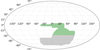 |
Fig. 1 Search region of this work (green) within the full DES footprint (green and gray). |
2.2 Data processing
In this study, we used data from DES DR2 covering the sky region with declination >−30°, as shown in Figure 1. This declination cut was adopted mainly due to limitations in our current storage and computational resources. The selected area was divided into six subregions, and the central coordinates for image retrieval were generated based on the ranges of right ascension (RA) and declination (Dec). Detailed information is given in Table 1.
Considering the large radius of UDGs, there is a possibility that UDGs located at the edges of images may be missed. To address this, we set up region overlaps when generating coordinates. Specifically, the field of view (FOV) for each image was set to 0.073 degrees (approximately 1001 × 1001 pixels), with a 100-pixel (∼ 26.3′′) overlap between adjacent images. Based on this setup, we calculated and generated the central coordinate catalog for all images to be downloaded in six subregions.
Dark Energy Survey images can be accessed through the NOIRLab Astro online platform (Fitzpatrick et al. 2014; Nikutta et al. 2020; Juneau et al. 2021), where they are provided in flexible image transport system (FITS) format. We retrieved the required image data using the simple image access (SIA) service provided by this platform. By specifying astronomical coordinates (RA, Dec) and a defined FOV size, we were able to obtain the deepest image cutouts and FITS files for various bands at the specified location and size. We selected data from the g, r, and i bands and synthesized RGB images using the Lupton method (Lupton et al. 2004). Ultimately, we successfully obtained 509 850 original images, with the number of images downloaded for each subregion shown in Table 1.
Sub-region details.
2.3 Initial training data
In current research, various definitions of UDGs exist, particularly regarding surface-brightness criteria. The mainstream definitions primarily fall into the following two categories.
Central surface brightness μ0,g ≥ 24 mag arcsec−2 based on Sérsic profile fitting. This metric depends on the Sérsic index n (e.g., van Dokkum et al. 2015; Bautista et al. 2023; Zaritsky et al. 2022; Lambert et al. 2024).
Average surface brightness 〈μeff,r〉 ≥ 24 mag arcsec−2 within the effective radius (e.g., van der Burg et al. 2016; Yagi et al. 2016; Janssens et al. 2017). This approach is argued to be more relevant for galaxy detectability and has the advantage of being independent of the Sérsic index when surface brightness and effective radius are fixed. For typical UDG parameters – Sérsic index n ∼ 1 (e.g., Koda et al. 2015; Román & Trujillo 2017; Yagi et al. 2016) and g−r color ∼ 0.6 (e.g., van der Burg et al. 2016; Zaritsky et al. 2023) this criterion can be approximately equivalent to 〈μeff,g〉 ≥ 24.6 mag arcsec−2 and μ0,g ≥ 23.5 mag arcsec−2 (Graham & Driver 2005).
In this work, we adopted the second convention and applied the following selection criteria:
〈μeff,g〉 ≥ 24.6 mag arcsec−2
reff ≥ 1.5 kpc.
The catalog provides the half-light radius (in arcseconds), but due to the lack of precise redshift measurements, we are unable to determine the intrinsic physical sizes of these galaxies. Therefore, we first calculated and selected objects with 〈μeff,g〉 ≥ 24.6 mag arcsec−2 and then performed morphological screening on these candidates; from 4083 low-surface-brightness galaxies, we selected UDG candidates with clear diffuse morphological features (excluding extremely faint targets that might be confused with background noise or artifacts). Ultimately, we chose 181 samples to construct the initial training set, with their axis-ratio distribution shown in Figure 2a. Figure 2b displays representative samples: the upper row shows typical examples with regular morphologies and relatively uniform brightness distributions, while the lower row presents samples with diverse morphological and structural features. All samples in this study were manually annotated using the LabelImg software.
3 Methods
3.1 The UDG detection model for DES (UDGnet-DES)
We developed UDGnet-DES for the detection of UDGs in DES. This model adopted the single-stage object-detection framework proposed in our previous work (Su et al. 2024). The object detection framework consists of four main modules: the image input module, feature-extraction module, feature-enhancement module, and output module. Through a multilevel feature-extraction and -enhancement strategy, combined with CSPDarknet (Wang et al. 2019) and PANet techniques (Liu et al. 2018), the model can effectively extract and integrate key features from the input images, thereby improving the accuracy of object detection and localization.
During the model-training phase, we applied various data-augmentation techniques to the images in the training set, including scaling, flipping, color-domain transformations, and Mosaic data augmentation (Bochkovskiy et al. 2020). The Mosaic data-augmentation method creates a new composite image by randomly scaling, cropping, and rearranging four images. For the initial training samples, UDGs were located at the center of the images. In our training, this method randomized and diversified the position of the targets within the composite images, thereby increasing the diversity of our training data (Figure 3). This augmentation method not only helps the model learn target features in different positions and backgrounds, it also effectively improves the model’s robustness and generalization ability, reducing the risk of overfitting.
The loss function of the model consists of three components: confidence loss, classification loss, and localization loss. The confidence loss and classification loss are calculated using the binary cross-entropy loss (BCELoss), while the localization loss is computed using generalized intersection over union (GIoU) (Rezatofighi et al. 2019). For optimization, the model uses the Adam optimization algorithm (Kingma & Ba 2017) to optimize the model parameters and improve the training performance. Ultimately, the trained model outputs the predicted results, which include the class of the predicted bounding box, its confidence score, and coordinate information.
3.2 Iterative training and search
As a data-driven model, UDGnet-DES requires a sufficient number of training samples to be effectively trained. Rich and diverse training data not only help the model better recognize the features of ultra-diffuse galaxies and improve its learning performance, they also enhance its generalization ability. Here, we adopted an iterative training approach. Using the initially established model to search for UDGs, the newly identified samples were added to the training set after morphological inspection and confirmation, and then the model was retrained, thereby gradually enhancing the effectiveness of the model.
We divided the dataset into training, validation, and test sets in a ratio of 8:1:1. In the initial division of training samples, the number of images in the training, validation, and test sets were 145, 18, and 18, respectively. We then input the divided dataset into the model for training. After 200 training epochs, the initial UDGnet-DES model was obtained, with a recall rate of 78.95% and a precision rate of 100%. Using this model to predict the first sky region (38 100 images), we obtained 380 images containing predicted bounding boxes. After visual inspection, 165 images containing new samples were selected. We excluded extremely faint objects during the visual inspection process. Such objects, owing to their small sizes and low luminosities, are difficult to reliably distinguish from faint stars, imaging artifacts, and background noise. Including them in the training set could lead the detection model to produce a large number of false positives. The same criterion was applied in the subsequent visual inspections.
Subsequently, we annotated 165 newly obtained images and added them to the training set, expanding it to 346 images. After 200 training epochs, we obtained the updated model. Using this model, we conducted a search in the second sky region; this resulted in 1385 images containing predicted bounding boxes, from which 624 were selected.
Next, we added the 624 newly obtained images to the training set, expanding it to 970 images, and retrained the model. Using this model, we predicted the images of the third sky region, resulting in 2499 images containing predicted bounding boxes. After visual inspection, 1319 images were selected.
Finally, we added 1319 new samples to the training set, expanding the training dataset to 2289 images. After 200 training epochs, we obtained the final UDGnet-DES model, achieving a recall rate of 96.28% and a precision level of 96.28% on the validation set. The newly labeled data added in each iteration allow the model to better adapt to the variations and diversity of the DES dataset, learning more diverse features from the continuously updated training set, which enhances its generalization ability. In this way, both the model’s performance and the efficiency of data utilization were effectively improved, leading to higher accuracy in identifying UDGs.
Using this model, we conducted a search in the northern region with declinations greater than −30° and identified 14 457 images containing 14 732 UDG candidates from a total of 509 850 images. As mentioned earlier, due to the overlapping of regions, these results include some duplicate sources. After deduplication, we obtained a final set of 11 470 preliminary UDG candidates.
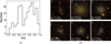 |
Fig. 2 (a) Axis-ratio distribution of 181 initial samples. (b) Example cutouts of six UDG candidate samples from initial training set. The RA and Dec coordinates of each galaxy center are provided in the lower left corners of the images. Each example corresponds to a 65.75′′ × 65.75′′ (250 × 250 pixels) sky region centered on the UDG. |
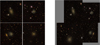 |
Fig. 3 Comparison of images before (left panel) and after Mosaic data augmentation (right panel). |
3.3 Selection based on parameters
The DES DR2 catalog, generated via its source-detection process, includes 691 483 608 different celestial objects. The information for each object includes centroid positions, shape parameters, processing flags, and various photometric measurements, among others. These data are stored in three tables of the DES DR2 catalog: DR2_MAIN, DR2_MAGNITUDE, and DR2_FLUX. DR2_MAIN is a summary table containing primary photometric measurements and non-photometric measurements.
To cross-match with the DR2_MAIN table and obtain various parameter information for the candidates, we converted the pixel coordinates of the 11470 preliminary UDG candidates into world coordinates. After obtaining the world coordinates for all candidates, we cross-matched these coordinates with the DR2_MAIN table using a 5-arcsec matching radius and retained all matches within this range (some coordinates may match multiple sources).
Then, we applied the following basic parameter criteria to filter the cross-matched sources. First, we excluded false detections and objects with photometric defects (such as saturated pixels or truncations) by applying the condition FLAG <4. Then, we removed objects with extended_class_coadd equal to 0 or 1, or extended_class_wavg equal to 0 or 1, as these are classified as stars and further remove potential stellar sources by restricting CLASS_STAR _0.4. Additionally, we set the minimum value of the axis ratio (B_IMAGE/A_IMAGE) to 0.3 to exclude gravitational lenses and elongated artifacts. Finally, we selected sources with magerr_auto < 0.2 in the g, r, and i bands to ensure that the magnitude measurements of the retained sources are accurate. After completing the above selection, in cases where multiple sources were matched to the same coordinates in the DES DR2, we retained the source that was closest in distance. Then, we calculated their mean effective surface brightness in the g band using formula (1) (Graham & Driver 2005) and selected 3346 candidates based on 〈μeff,g〉 ≥ 24.6 mag arcsec−2:
 (1)
(1)
To convert the effective radius of the candidates into physical sizes, we cross-matched the filtered results with the redshift data from the Simbad database (Wenger et al. 2000) and the Dark Energy Camera Legacy Survey (DECaLS; Blum et al. 2016), obtaining spectroscopic redshift information for 62 candidates. We then calculated the angular diameter distance and determined the actual physical radius of the candidates. Finally, by selecting sources with an effective radius greater than 1.5 kpc, we identified 39 UDG samples that satisfy both the surfacebrightness and effective-radius criteria. The properties of these samples are shown in Appendix A, and Figure 4a displays some representative examples.
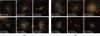 |
Fig. 4 Example images of candidate UDGs detected by UDGnet-DES model (250 × 250 pixels). (a) Examples of six UDGs from the 39 UDGs, and (b) examples of six UDG candidates from the 2952 candidate UDGs. |
3.4 Visual inspection
To ensure the quality of the UDG candidate samples, we created cutouts of 250′′ × 250′′ centered on each candidate for visual inspection. Of the 3346 UDG candidates obtained earlier, 3284 had no cross-matched redshift data; we conducted a visual inspection of them and implemented a detailed classification system for all candidate objects, categorizing them into four distinct classes based on their morphological characteristics and likelihood of being genuine UDGs. These are listed below.
AS (smooth UDG candidates): we identified 859 objects that exhibit smooth surface-brightness distributions and regular, nearly elliptical shapes. These candidates are considered to be definitive UDGs with high confidence; they are characterized by a regular shape and homogeneous stellar distributions.
AUS (unsmooth UDG candidates): 2093 objects were classified as definitive UDGs, but with irregular morphologies; they exhibit non-smooth surface-brightness distributions or asymmetric shapes. These candidates, while clearly ultra-diffuse in nature, show structural irregularities that may indicate arms, interactions, or ongoing star formation processes, or internal disturbances.
B (possible UDGs): 220 objects were categorized as possible UDG candidates, where the classification remains uncertain due to ambiguous morphological features or small sizes. These objects meet some but not all criteria with high confidence. They are either too small or are likely irregulars, draft ellipticals, or small spiral galaxies, usually with denser cores. While this sample may include some sources that are not genuine UDGs, we cannot definitively exclude them without accurate redshift measurements.
C (non-UDGs): the remaining objects were classified as definitively not UDGs; they often have no features of UDGs, including artifacts (e.g., halos, CCD defects), and non-UDG objects (e.g., faint tidal tails, parts of spiral arms).
We retained the sources in the AS and AUS categories, constructing a catalog of 2952 UDG candidates. The sequential selection steps are outlined in Figure 5, and six representative examples are displayed in Figure 4b.
4 UDG properties
We finally obtained a catalog of 2991 UDG samples from DES DR2, which includes 39 spectroscopically confirmed UDGs and 2952 UDG candidates. In this section, we describe the properties of these samples in detail.
4.1 Structural parameters of UDG samples
Figures 6a–6d show histograms of the color (g-i), mean effective surface brightness in the g band (〈μeff,g〉), and axis ratio (q) for the 39 UDGs. We divided UDGs into two groups: blue UDGs (g−i<0.6) and red UDGs (g−i>0.6). Figure 6a displays the number distribution of UDGs in different color groups. Overall, the color indices of the samples are concentrated between 0.3 and 0.8. Among the 39 samples, 24 are blue UDGs and 15 are red UDGs, with blue UDGs outnumbering red ones. The distribution of color indices may be closely related to the star formation history, stellar populations, dust content, and other physical properties of UDGs. Blue UDGs may exhibit stronger star formation activity, while red UDGs likely have less star formation activity.
As shown in Figure 6b, the distribution of the mean effective surface brightness 〈μeff,g〉 is approximately 24.6− 26 mag arcsec−2, with most samples falling within the 24.6− 25 mag arcsec−2 range. This indicates that the surface brightness of these samples is relatively concentrated and mainly clustered in the brighter brightness intervals. Within the range of surface brightness under 25 mag arcsec−2, the number of blue UDGs is significantly higher than that of red ones, whereas in the range above 25 mag arcsec−2, the numbers of both are comparable. This distribution trend suggests that, compared to red UDGs, blue UDGs may generally have higher surface brightness. These results are consistent with recent findings concerning UDGs from the Dark Energy Spectroscopic Instrument (DESI) Southern traditional imaging survey (Zaritsky et al. 2022). However, due to the limited sample size, the statistical significance of these results still requires further verification.
Figure 6c shows that the axis ratios of all samples are distributed between 0.4 and 1. The average axis ratios of both blue UDGs and red UDGs are biased toward larger values (0.718 and 0.742, respectively), indicating that most of these samples exhibit near-circular shapes. This suggests that red UDGs tend to have shapes that are closer to circular compared to blue UDGs.
Figure 6d shows the distribution of effective radius (re) for 37 UDGs. It is worth noting that we excluded two UDGs with exceptionally large redshift values whose physical radii exceeded 50 kpc in order to clearly display the overall distribution. As seen in the figure, most of the samples have an effective radius smaller than 6 kpc, which is consistent with the findings of van Dokkum et al. (2015), Iodice et al. (2020), and Lee et al. (2017). The median effective radius of these UDGs is 4.42 kpc, with a peak around 1.5 kpc for the blue UDGs and a peak around 5 kpc for the red ones. This difference suggests that blue UDGs generally have smaller effective radius compared to red ones, potentially indicating more compact structures. For the seven sources with exceptionally large physical sizes ((re) > 10 kpc), cross-matching with the Simbad database and multiple rounds of visual inspection confirm that these targets are all classified as either normal galaxies or low-surface-brightness galaxies. Among them, five sources have relatively large redshifts (z > 0.28), while the anomalous sizes of the remaining two low-redshift sources may result from fitting biases due to their extremely low surface brightnesses.
The histograms of color (g-i), average effective surface brightness in the g-band (〈μeff,g〉), axis ratio (q), and effective radius (re) for the 2952 UDG candidate samples are shown in Figures 7a–7d. From the statistical analysis of the data shown in Figure 7a, we found that there are 1589 blue candidates and 1363 red candidates, indicating that the blue candidates are more numerous. Moreover, the distribution of the candidates still follows a pattern of fewer numbers at the extremes and more in the middle, similar to the results in Figure 6a.
Figure 7b shows that for surface-brightness values under 25.4 mag arcsec−2, the number of blue candidates is significantly higher than that of red candidates, while for values greater than 25.4 mag arcsec−2, the red candidates outnumber the blue ones. This distribution pattern matches that shown in Figure 6b, and the surface brightness of the blue UDG samples is more concentrated in the brighter range. Furthermore, by plotting the radius-magnitude diagram for all 2991 samples (including 39 UDGs with redshift information and 2952 UDG candidates without redshift), as shown in Figure 8, this characteristic is more clearly visualized. From the diagram, it can be observed that the blue UDG candidates are primarily distributed between the dashed black line and the dashed green line, corresponding to a surface-brightness concentration between 24.6 and 25.6 mag arcsec−2. In the region above the dashed green line (corresponding to surface brightness greater than 25.6), the number of red UDG candidates is much higher than that of blue ones. These results further confirm the difference in surface brightness between the blue and red UDG candidates.
As shown in Figure 7c, the axis ratios of these candidates are distributed between 0.3 and 1. Further analysis showed that the mean axis ratio for the blue candidates was approximately 0.72, while the mean for the red candidates was approximately 0.75, which aligned with the results in Figure 6c. Additionally, in Figure 7d, the effective radii of these candidates are mostly concentrated within 10′′, with only a few candidates having an effective radius greater than 10′′. Notably, the blue candidates show a stronger tendency to be concentrated in the smaller radius range.
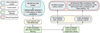 |
Fig. 5 Sequential selection steps used to find the UDG candidates. |
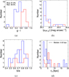 |
Fig. 6 Distribution of structural parameters for 39 UDGs: g-i color (panel a); average effective surface brightness (panel b); axis ratio (panel c); and effective radius (panel d). The blue histogram shows the distribution of blue UDGs, while the red histogram shows the distribution of red UDGs. The proportion of blue UDGs and red UDGs is labeled in the upper left corner of panel a. |
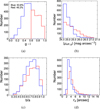 |
Fig. 7 Distribution of structural parameters for 2952 UDG candidates: g-i color (panel a); average effective surface brightness (panel b); axis ratio (panel c); and effective radius (panel d). The blue histograms represent the distribution of blue candidates, while the red histograms represent the distribution of red candidates. The top left corner of panel a indicates the proportions of blue and red candidates. |
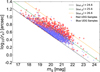 |
Fig. 8 Radius-magnitude diagram for all UDG samples(2991 in total). Red UDG samples are represented by red circles, and blue UDG samples are represented by blue triangles. The dashed line corresponds to the average effective surface brightness in the g band. |
4.2 Spatial distributions of UDG samples
The spatial distribution of all red and blue UDG samples identified in this study is shown in Figure 9. All samples exhibit a broad distribution in the northern region of the DES sky map. Among them, red samples tend to cluster together, while blue samples show a more uniform distribution across the sky, which may be related to the origins of UDGs. Red UDG samples are likely to be members of galaxy clusters or groups, while blue UDG samples are more likely to be distributed in the field.
In Figure 9, the red UDG samples within the declination range of −24° to −16° exhibit a notable clustering feature (as indicated by the green box). This region contains known substructures (the Eridanus constellation). Further investigation reveals the presence of galaxy cluster Abell 194 at coordinates 21.4200°,−1.4072° (marked by a green circle) and galaxy cluster RXC J0340.1-1835 at coordinates 55.0475°,−18.5875° (marked by a black circle). The red UDG candidates in the vicinity of these regions are likely to be dynamically or evolutionarily associated with these galaxy clusters, suggesting potential formation mechanisms or evolutionary pathways of UDGs in cluster environments.
5 Comparison with SMUDGes sample
To evaluate the differences between the UDG candidates identified in our search and those from previous studies, we compared our catalog with the SMUDGes catalog (Zaritsky et al. 2022). The SMUDGes catalog is derived from a search conducted in the southern portion of the DESI Legacy Imaging Surveys. It employs a multistage processing pipeline that includes wavelet-based source detection, structural parameter fitting with GALFIT, rigorous screening for imaging artifacts and Galactic cirrus, and a final classification step using a convolutional neural network. The resulting catalog contains 5598 UDG candidates, defined by the selection criteria μ0, g > 24 mag arcsec−2 and re>5.3′′. Among them, 938 UDG candidates lie within our study region, and a comparison of their sky distribution with our catalog is shown in Figure 10.
We cross-matched our catalog with SMUDGes using a matching radius of eight arcseconds. Considering potential positional offsets in the central coordinates of larger targets and possible misidentifications caused by coordinate shifts between neighboring objects, we conducted visual inspections for matches with separations between four and eight arcseconds to eliminate false matches. We finally confirmed 501 reliable counterparts common to both catalogs. Among these matched sources, the ratio of AS to AUS classifications is approximately 1.6, indicating a selection preference within the SMUDGes catalog for UDGs with smoother morphologies. Figure 11 compares the surface-brightness distribution of the matched sources with that of our catalog. The matched sources are mainly distributed at fainter surface brightness levels, indicating that they correspond to the fainter end of our UDG candidates.
Within the same region, our catalog includes 2490 newly detected UDG candidates that are not present in the SMUDGes catalog. Among these newly identified candidates, the number of UDGs in the AUS subset is approximately three times that in the AS subset. This result indicates that our method is capable of identifying many UDGs with non-smooth, structured morphologies that are often missed by traditional searches. These morphologically complex candidates provide valuable insights into the formation mechanisms of dark galaxies, as their structural diversity may reflect different origin scenarios such as tidal stripping or dissipative formation processes. In addition, 437 UDG candidates from the SMUDGes sample were not recovered in our catalog. Visual inspection shows that the majority of these sources (∼ 75%) are extremely faint systems lacking discernible internal structure. As described in Sections 2.3 and 3.2, such extremely faint objects were excluded during the construction of our training set to avoid confusion with artifacts.
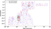 |
Fig. 9 Sky distribution of red UDG samples (red dots) and blue UDG samples (blue dots) identified in this study (2991 in total). The green circle marks the location of the Abell 194 galaxy cluster (RA=21.4200°, Dec=−1.4072°), and the black circle marks the location of the RXC J0340.1-1835 galaxy cluster (RA =55.0475°, Dec =−18.5875°). The green box highlights the region where red UDG samples show a significant clustering feature, with Dec values between −24° and −16°. |
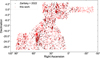 |
Fig. 10 Spatial distribution of sources from this catalog and that of Zaritsky et al. (2022). |
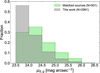 |
Fig. 11 Comparison of surface-brightness distributions between 501 matched sources and the full samples in this study. |
6 Conclusion
We present UDGnet-DES, a deep-learning framework for ultra-diffuse galaxy detection in DES imaging. Leveraging CSPDarknet and PANet architectures with an iterative training scheme, the model achieves a recall and precision level of 96.28%, efficiently identifying 11 470 preliminary candidates from 509850 DES DR2 images. Compared with traditional, manually intensive methods, UDGnet-DES offers a highly automated, scalable solution well suited to the era of large astronomical surveys, and it provides a transferable framework for identifying other low-surface-brightness systems.
Our final catalog contains 2991 UDG candidates, including 39 with spectroscopic redshifts. The catalog spans both smooth and morphologically irregular systems, enabling a comprehensive study of UDG diversity. Statistical analysis reveals clear distinctions between blue and red UDGs: blue systems exhibit higher surface brightness and a more uniform spatial distribution, while red systems show pronounced clustering. Comparison with the SMUDGes catalog demonstrates a significant advantage of our deep-learning approach: its enhanced sensitivity to UDGs exhibiting non-smooth, structured morphologies. These results provide new observational constraints on UDG formation pathways, evolutionary processes, and environmental dependencies.
Data availability
The full catalog is available at the CDS via https://cdsarc.cds.unistra.fr/viz-bin/cat/J/A+A/706/A35.
Acknowledgements
This study was supported by the National Natural Science Foundation of China (NSFC) grant no. 12573109, Shandong Province Natural Science Foundation (grant Nos. ZR2022MA089, ZR2022MA076, ZR2024MA063 and ZR2025MS06) and the China Manned Space Program with grant Nos. CMS-CSST-2025-A06, CMS-CSST-2021-B05 and CMS-CSST-2021-A08. We thank the DES team for the released DES images and parameter catalog. This project used public archival data from the Dark Energy Survey (DES). Funding for the DES Projects has been provided by the U.S. Department of Energy, the U.S. National Science Foundation, the Ministry of Science and Education of Spain, the Science and Technology FacilitiesCouncil of the United Kingdom, the Higher Education Funding Council for England, the National Center for Supercomputing Applications at the University of Illinois at Urbana-Champaign, the Kavli Institute of Cosmological Physics at the University of Chicago, the Center for Cosmology and Astro-Particle Physics at the Ohio State University, the Mitchell Institute for Fundamental Physics and Astronomy at Texas A&M University, Financiadora de Estudos e Projetos, Fundação Carlos Chagas Filho de Amparo à Pesquisa do Estado do Rio de Janeiro, Conselho Nacional de Desenvolvimento Científico e Tecnológico and the Ministério da Ciência, Tecnologia e Inovação, the Deutsche Forschungsgemeinschaft, and the Collaborating Institutions in the Dark Energy Survey. This research uses services or data provided by the Astro Data Lab, which is part of the Community Science and Data Center (CSDC) Program of NSF NOIRLab. NOIRLab is operated by the Association of Universities for Research in Astronomy (AURA), Inc. under a cooperative agreement with the U.S. National Science Foundation. The DESI Legacy Imaging Surveys consist of three individual and complementary projects: the Dark Energy Camera Legacy Survey (DECaLS), the Beijing-Arizona Sky Survey (BASS), and the Mayall z-band Legacy Survey (MzLS). The complete acknowledgments can be found at https://www.legacysurvey.org/acknowledgment/. This research has made use of the SIMBAD database, CDS, and the CDS cross-match service, Strasbourg Astronomical Observatory, France.
References
- Abbott, T. M. C., Abdalla, F. B., Allam, S., et al. 2018, ApJS, 239, 18 [Google Scholar]
- Abbott, T. M. C., Adamów, M., Aguena, M., et al. 2021, ApJS, 255, 20 [NASA ADS] [CrossRef] [Google Scholar]
- Abraham, R. G., & van Dokkum, P. G., 2014, PASP, 126, 55 [Google Scholar]
- Amorisco, N. C., & Loeb, A., 2016, MNRAS, 459, L51 [NASA ADS] [CrossRef] [Google Scholar]
- Bautista, J. M. G., Koda, J., Yagi, M., Komiyama, Y., & Yamanoi, H., 2023, ApJS, 267, 10 [NASA ADS] [CrossRef] [Google Scholar]
- Blum, R. D., Burleigh, K., Dey, A., et al. 2016, in American Astronomical Society Meeting Abstracts, 228, 317.01 [Google Scholar]
- Bochkovskiy, A., Wang, C.-Y., & Liao, H.-Y. M., 2020, arXiv e-prints [arXiv:2004.10934] [Google Scholar]
- Caldwell, N., & Bothun, G. D., 1987, AJ, 94, 1126 [Google Scholar]
- Carleton, T., Errani, R., Cooper, M., et al. 2019, MNRAS, 485, 382 [NASA ADS] [CrossRef] [Google Scholar]
- Chan, T. K., Kereš, D., Wetzel, A., et al. 2018, MNRAS, 478, 906 [NASA ADS] [CrossRef] [Google Scholar]
- Chilingarian, I. V., Afanasiev, A. V., Grishin, K. A., Fabricant, D., & Moran, S., 2019, ApJ, 884, 79 [NASA ADS] [CrossRef] [Google Scholar]
- Cohen, Y., van Dokkum, P., Danieli, S., et al. 2018, ApJ, 868, 96 [Google Scholar]
- Dalcanton, J. J., Spergel, D. N., Gunn, J. E., Schmidt, M., & Schneider, D. P., 1997, AJ, 114, 635 [Google Scholar]
- Dey, A., Schlegel, D. J., Lang, D., et al. 2019, AJ, 157, 168 [Google Scholar]
- Fitzpatrick, M. J., Olsen, K., Economou, F., et al. 2014, SPIE Conf. Ser., 9149, 91491T [Google Scholar]
- Flaugher, B., 2005, Int. J. Mod. Phys. A, 20, 3121 [Google Scholar]
- Flaugher, B., Diehl, H. T., Honscheid, K., et al. 2015, AJ, 150, 150 [Google Scholar]
- Gannon, J. S., Dullo, B. T., Forbes, D. A., et al. 2021, MNRAS, 502, 3144 [Google Scholar]
- Gannon, J. S., Forbes, D. A., Romanowsky, A. J., et al. 2022, MNRAS, 510, 946 [Google Scholar]
- Graham, A. W., & Driver, S. P., 2005, PASA, 22, 118 [NASA ADS] [CrossRef] [Google Scholar]
- Habas, R., Marleau, F. R., Duc, P.-A., et al. 2020, MNRAS, 491, 1901 [NASA ADS] [Google Scholar]
- Honscheid, K., & DePoy, D. L., 2008, arXiv e-prints [arXiv:0810.3600] [Google Scholar]
- Impey, C., Bothun, G., & Malin, D., 1988, ApJ, 330, 634 [Google Scholar]
- Iodice, E., Cantiello, M., Hilker, M., et al. 2020, A&A, 642, A48 [EDP Sciences] [Google Scholar]
- Janssens, S., Abraham, R., Brodie, J., et al. 2017, ApJ, 839, L17 [NASA ADS] [CrossRef] [Google Scholar]
- Jones, M. G., Sand, D. J., Karunakaran, A., et al. 2024, ApJ, 966, 93 [NASA ADS] [CrossRef] [Google Scholar]
- Juneau, S., Olsen, K., Nikutta, R., Jacques, A., & Bailey, S., 2021, Comput. Sci. Eng., 23, 15 [Google Scholar]
- Karunakaran, A., & Zaritsky, D., 2023, MNRAS, 519, 884 [Google Scholar]
- Karunakaran, A., Motiwala, K., Spekkens, K., et al. 2024, ApJ, 975, 91 [Google Scholar]
- Kingma, D. P., & Ba, J., 2017, Adam: A Method for Stochastic Optimization [Google Scholar]
- Koda, J., Yagi, M., Yamanoi, H., & Komiyama, Y., 2015, ApJ, 807, L2 [NASA ADS] [CrossRef] [Google Scholar]
- Lambert, M., Khim, D. J., Zaritsky, D., & Donnerstein, R., 2024, AJ, 167, 61 [NASA ADS] [CrossRef] [Google Scholar]
- Lee, M. G., Kang, J., Lee, J. H., & Jang, I. S., 2017, ApJ, 844, 157 [CrossRef] [Google Scholar]
- Lee, J. H., Kang, J., Lee, M. G., & Jang, I. S., 2020, ApJ, 894, 75 [NASA ADS] [CrossRef] [Google Scholar]
- Leisman, L., Haynes, M. P., Janowiecki, S., et al. 2017, ApJ, 842, 133 [NASA ADS] [CrossRef] [Google Scholar]
- Lim, S., Peng, E. W., Côté, P., et al. 2018, ApJ, 862, 82 [Google Scholar]
- Liu, S., Qi, L., Qin, H., Shi, J., & Jia, J., 2018, arXiv e-prints [arXiv:1803.01534] [Google Scholar]
- Lupton, R., Blanton, M. R., Fekete, G., et al. 2004, PASP, 116, 133 [NASA ADS] [CrossRef] [Google Scholar]
- Martin, G., Kaviraj, S., Laigle, C., et al. 2019, MNRAS, 485, 796 [NASA ADS] [CrossRef] [Google Scholar]
- Martínez-Delgado, D., Läsker, R., Sharina, M., et al. 2016, AJ, 151, 96 [CrossRef] [Google Scholar]
- Merritt, A., van Dokkum, P., Danieli, S., et al. 2016, ApJ, 833, 168 [NASA ADS] [CrossRef] [Google Scholar]
- Montes, M., Trujillo, I., Karunakaran, A., et al. 2024, A&A, 681, A15 [NASA ADS] [CrossRef] [EDP Sciences] [Google Scholar]
- Nikutta, R., Fitzpatrick, M., Scott, A., & Weaver, B., 2020, Astron. Comput., 33, 100411 [Google Scholar]
- Prole, D. J., van der Burg, R. F. J., Hilker, M., & Davies, J. I., 2019, MNRAS, 488, 2143 [NASA ADS] [Google Scholar]
- Rezatofighi, H., Tsoi, N., Gwak, J., et al. 2019, arXiv e-prints [arXiv:1902.09630] [Google Scholar]
- Román, J., & Trujillo, I., 2017, MNRAS, 468, 4039 [Google Scholar]
- Sales, L. V., Navarro, J. F., Peñafiel, L., et al. 2020, MNRAS, 494, 1848 [Google Scholar]
- Sandage, A., & Binggeli, B., 1984, AJ, 89, 919 [Google Scholar]
- Sengupta, C., Scott, T. C., Chung, A., & Wong, O. I., 2019, MNRAS, 488, 3222 [NASA ADS] [CrossRef] [Google Scholar]
- Sevilla-Noarbe, I., Bechtol, K., Carrasco Kind, M., et al. 2021, ApJS, 254, 24 [NASA ADS] [CrossRef] [Google Scholar]
- Somalwar, J. J., Greene, J. E., Greco, J. P., et al. 2020, ApJ, 902, 45 [NASA ADS] [CrossRef] [Google Scholar]
- Su, H., Yi, Z., Liang, Z., et al. 2024, MNRAS, 528, 873 [NASA ADS] [CrossRef] [Google Scholar]
- Tanoglidis, D., Drlica-Wagner, A., Wei, K., et al. 2021, ApJS, 252, 18 [Google Scholar]
- Thuruthipilly, H., Junais, Pollo, A., et al. 2024, A&A, 682, A4 [NASA ADS] [CrossRef] [EDP Sciences] [Google Scholar]
- Toloba, E., Lim, S., Peng, E., et al. 2018, ApJ, 856, L31 [CrossRef] [Google Scholar]
- van der Burg, R. F. J., Muzzin, A., & Hoekstra, H., 2016, A&A, 590, A20 [NASA ADS] [CrossRef] [EDP Sciences] [Google Scholar]
- van Dokkum, P. G., Abraham, R., Merritt, A., et al. 2015, ApJ, 798, L45 [NASA ADS] [CrossRef] [Google Scholar]
- van Dokkum, P., Abraham, R., Brodie, J., et al. 2016, ApJ, 828, L6 [Google Scholar]
- Venhola, A., Peletier, R., Laurikainen, E., et al. 2017, A&A, 608, A142 [NASA ADS] [CrossRef] [EDP Sciences] [Google Scholar]
- Venhola, A., Peletier, R. F., Salo, H., et al. 2022, A&A, 662, A43 [NASA ADS] [CrossRef] [EDP Sciences] [Google Scholar]
- Wang, C.-Y., Liao, H.-Y. M., Yeh, I.-H., et al. 2019, arXiv e-prints [arXiv:1911.11929] [Google Scholar]
- Wenger, M., Ochsenbein, F., Egret, D., et al. 2000, A&AS, 143, 9 [NASA ADS] [Google Scholar]
- Wittmann, C., Lisker, T., Ambachew Tilahun, L., et al. 2017, MNRAS, 470, 1512 [Google Scholar]
- Yagi, M., Koda, J., Komiyama, Y., & Yamanoi, H., 2016, ApJS, 225, 11 [CrossRef] [Google Scholar]
- Zaritsky, D., 2017, MNRAS, 464, L110 [NASA ADS] [CrossRef] [Google Scholar]
- Zaritsky, D., Donnerstein, R., Dey, A., et al. 2019, ApJS, 240, 1 [Google Scholar]
- Zaritsky, D., Donnerstein, R., Karunakaran, A., et al. 2022, ApJS, 261, 11 [NASA ADS] [CrossRef] [Google Scholar]
- Zaritsky, D., Donnerstein, R., Dey, A., et al. 2023, ApJS, 267, 27 [NASA ADS] [CrossRef] [Google Scholar]
Appendix A Additional Table
The catalog for the 39 UDGs.
All Tables
All Figures
|
Fig. 1 Search region of this work (green) within the full DES footprint (green and gray). |
| In the text | |
|
Fig. 2 (a) Axis-ratio distribution of 181 initial samples. (b) Example cutouts of six UDG candidate samples from initial training set. The RA and Dec coordinates of each galaxy center are provided in the lower left corners of the images. Each example corresponds to a 65.75′′ × 65.75′′ (250 × 250 pixels) sky region centered on the UDG. |
| In the text | |
|
Fig. 3 Comparison of images before (left panel) and after Mosaic data augmentation (right panel). |
| In the text | |
|
Fig. 4 Example images of candidate UDGs detected by UDGnet-DES model (250 × 250 pixels). (a) Examples of six UDGs from the 39 UDGs, and (b) examples of six UDG candidates from the 2952 candidate UDGs. |
| In the text | |
|
Fig. 5 Sequential selection steps used to find the UDG candidates. |
| In the text | |
|
Fig. 6 Distribution of structural parameters for 39 UDGs: g-i color (panel a); average effective surface brightness (panel b); axis ratio (panel c); and effective radius (panel d). The blue histogram shows the distribution of blue UDGs, while the red histogram shows the distribution of red UDGs. The proportion of blue UDGs and red UDGs is labeled in the upper left corner of panel a. |
| In the text | |
|
Fig. 7 Distribution of structural parameters for 2952 UDG candidates: g-i color (panel a); average effective surface brightness (panel b); axis ratio (panel c); and effective radius (panel d). The blue histograms represent the distribution of blue candidates, while the red histograms represent the distribution of red candidates. The top left corner of panel a indicates the proportions of blue and red candidates. |
| In the text | |
|
Fig. 8 Radius-magnitude diagram for all UDG samples(2991 in total). Red UDG samples are represented by red circles, and blue UDG samples are represented by blue triangles. The dashed line corresponds to the average effective surface brightness in the g band. |
| In the text | |
|
Fig. 9 Sky distribution of red UDG samples (red dots) and blue UDG samples (blue dots) identified in this study (2991 in total). The green circle marks the location of the Abell 194 galaxy cluster (RA=21.4200°, Dec=−1.4072°), and the black circle marks the location of the RXC J0340.1-1835 galaxy cluster (RA =55.0475°, Dec =−18.5875°). The green box highlights the region where red UDG samples show a significant clustering feature, with Dec values between −24° and −16°. |
| In the text | |
|
Fig. 10 Spatial distribution of sources from this catalog and that of Zaritsky et al. (2022). |
| In the text | |
|
Fig. 11 Comparison of surface-brightness distributions between 501 matched sources and the full samples in this study. |
| In the text | |
Current usage metrics show cumulative count of Article Views (full-text article views including HTML views, PDF and ePub downloads, according to the available data) and Abstracts Views on Vision4Press platform.
Data correspond to usage on the plateform after 2015. The current usage metrics is available 48-96 hours after online publication and is updated daily on week days.
Initial download of the metrics may take a while.