| Issue |
A&A
Volume 706, February 2026
|
|
|---|---|---|
| Article Number | A106 | |
| Number of page(s) | 12 | |
| Section | Astrophysical processes | |
| DOI | https://doi.org/10.1051/0004-6361/202556971 | |
| Published online | 03 February 2026 | |
Mini-supernovae from white dwarf–neutron star mergers: Viewing-angle-dependent spectra and light curves
1
Department of Astronomy, School of Physics, Peking University Beijing 100871, China
2
Kavli Institute for Astronomy and Astrophysics, Peking University Beijing 100871, China
3
The Hong Kong Institute for Astronomy and Astrophysics, The University of Hong Kong Pokfulam Road Hong Kong, People’s Republic of China
4
Department of Physics, The University of Hong Kong Pokfulam Road Hong Kong, People’s Republic of China
5
School of Physics and Astronomy, Monash University Clayton Victoria 3800, Australia
6
OzGrav: The ARC Centre of Excellence for Gravitational Wave Discovery Clayton Victoria 3800, Australia
7
National Astronomical Observatories, Chinese Academy of Sciences Beijing 100012, China
8
The Nevada Center for Astrophysics and Department of Physics and Astronomy, University of Nevada Las Vegas NV 89154, USA
★ Corresponding authors: This email address is being protected from spambots. You need JavaScript enabled to view it.
; This email address is being protected from spambots. You need JavaScript enabled to view it.
; This email address is being protected from spambots. You need JavaScript enabled to view it.
Received:
25
August
2025
Accepted:
8
December
2025
Abstract
Context. Unstable mass transfer may occur during white dwarf–neutron star (WD–NS) mergers, in which the WD can be tidally disrupted and form an accretion disk around the NS. Such an accretion disk can produce unbound wind ejecta with synthesized 56Ni mixed in. Numerical simulations reveal that this unbound ejecta should be strongly polar-dominated, which may cause the subsequent radioactive-powered thermal transient to be viewing-angle-dependent–an issue that has so far received limited investigation.
Aims. We investigated how the intrinsically nonspherical geometry of WD–NS wind ejecta affects the viewing-angle dependence of the thermal transients.
Methods. Using a two-dimensional axisymmetric ejecta configuration and incorporating heating from the radioactive decay of 56Ni, we employed a semi-analytical discretization scheme to simulate the observed viewing-angle-dependent photospheric evolution, as well as the resulting spectra and light curves.
Results. The observed photosphere evolves over time and shows a strong dependence on the viewing angle: off-axis observers can see deeper, hotter inner layers of the ejecta and larger projected photospheric areas compared to on-axis observers. For a fiducial WD–NS merger producing 0.3 M⊙ of ejecta and 0.01 M⊙ of synthesized 56Ni, the resulting peak optical absolute magnitudes of the transient span from ≃ − 12 mag along the polar direction to ≃ − 16 mag along the equatorial direction, corresponding to luminosities of ∼1040–1042 erg s−1. The typical peak timescales are expected to be 3–10 d.
Conclusions. We present the first exploration of the viewing-angle effect on WD–NS merger transients. Since their ejecta composition and energy sources resemble those of supernovae, yet WD–NS merger transients are dimmer and evolve more rapidly, we propose using “mini-supernovae” to describe the thermal emission following WD–NS mergers. Our study highlights the critical role of geometry in the interpretation of WD–NS mini-supernovae and motivates further exploration of their diversity in observation.
Key words: radiation: dynamics / radiation mechanisms: thermal / radiative transfer / binaries: close / white dwarfs / stars: winds / outflows
© The Authors 2026
 Open Access article, published by EDP Sciences, under the terms of the Creative Commons Attribution License (https://creativecommons.org/licenses/by/4.0), which permits unrestricted use, distribution, and reproduction in any medium, provided the original work is properly cited.
This article is published in open access under the Subscribe to Open model. This email address is being protected from spambots. You need JavaScript enabled to view it. to support open access publication.
1. Introduction
Among the various types of double-compact-object (DCO) mergers, systems that contain at least one neutron star (NS) are of particular interest, especially as promising progenitors of diverse electromagnetic (EM) transients and as detectable gravitational-wave (GW) sources. This interest was greatly enhanced by the detection of the first GW binary neutron star (BNS) merger, GW170817 (Abbott et al. 2017c), accompanied by the short-duration gamma-ray burst (SGRB) GRB 170817A (Abbott et al. 2017b; Goldstein et al. 2017; Savchenko et al. 2017; Zhang et al. 2018) and the kilonova transient AT 2017gfo (Andreoni et al. 2017; Arcavi et al. 2017; Chornock 2017; Coulter et al. 2017; Cowperthwaite et al. 2017; Díaz et al. 2017; Drout et al. 2017; Evans et al. 2017; Hu 2017; Kasliwal et al. 2017; Kilpatrick et al. 2017; Lipunov et al. 2017; McCully et al. 2017; Nicholl et al. 2017b; Pian et al. 2017; Pozanenko et al. 2018; Shappee et al. 2017; Smartt et al. 2017; Soares-Santos et al. 2017; Tanvir et al. 2017; Troja et al. 2017; Utsumi et al. 2017; Valenti et al. 2017). Such a multimessenger detection of a BNS GW event and its associated EM counterparts provides direct evidence that BNS mergers can drive relativistic jets to power SGRBs (Paczynski 1986; Eichler et al. 1989; Paczynski 1991; Narayan et al. 1992; Zhang 2018) and eject neutron-rich outflows undergoing r-process nucleosynthesis to produce kilonova emissions (Li & Paczynski 1998; Metzger et al. 2010; Metzger 2020). Moreover, this event has offered a unique opportunity to probe dense-matter physics and test gravity under extreme conditions (Abbott et al. 2017a, 2018, 2019; Shao et al. 2017; Sathyaprakash et al. 2019; Zhao et al. 2019; Shao & Yagi 2022). Thus, GW170817 is widely regarded as a milestone event in astronomy and fundamental physics (Abbott et al. 2017d; Nakar 2020; Radice et al. 2020; Margutti & Chornock 2021; Bian et al. 2021; Nicholl & Andreoni 2025).
In addition to BNS mergers, neutron star–black hole (NS–BH) mergers are also expected to produce observable SGRBs and kilonovae (Paczynski 1986; Eichler et al. 1989; Paczynski 1991; Narayan et al. 1992; Zhang 2018). Although several NS–BH GW events and candidates were reported during the LIGO-Virgo-KAGRA (LVK) Collaboration’s third and fourth observing runs (O3 and O4; Abbott et al. 2021a,b, 2023a; Abac et al. 2024), follow-up campaigns have, to date, failed to identify any convincing EM counterparts (e.g., Gomez et al. 2019; Andreoni et al. 2020; Ackley et al. 2020; Kawaguchi et al. 2020a; Han et al. 2020; Kyutoku et al. 2020), in particular, the expected kilonovae. Such non-detections could result from the large distances of these events, incomplete coverage of the large GW localization regions, or the fact that many NS–BH mergers are direct plunges, leaving little or no ejecta (e.g., Abbott et al. 2021b; Zhu et al. 2021b,a, 2024; Fragione 2021; Abac et al. 2024).
In recent years, several kilonova-like transients have been unexpectedly discovered in association with long-duration GRBs (LGRBs), for example, LGRB 211211A (Rastinejad et al. 2022; Yang et al. 2022; Troja et al. 2022) and LGRB 230307A (Levan et al. 2024; Yang et al. 2024; Gillanders & Smartt 2025). These discoveries challenge the classical GRB classification, since phenomenological LGRBs are typically thought to originate from the core collapse of massive stars, which are usually accompanied by broad-lined type Ic supernovae (SNe; Woosley 1993; Paczynski 1998; Woosley et al. 1999; MacFadyen & Woosley 1999; Metzger et al. 2010; Zhang 2018; Metzger 2020), rather than by kilonovae associated with DCO mergers. If these merger-driven LGRBs indeed arise from BNS or NS–BH mergers, the observed kilonova emission can be naturally interpreted; however, their long prompt-emission durations remain difficult to reconcile with the current understanding of jet production in such DCO mergers, where the accretion episodes that launch jets are expected to be relatively short (Narayan et al. 1992; Yuan & Zhang 2012; Zhang 2018, 2025). Together, these theoretical and observational tensions suggest that merger-driven LGRBs may constitute a distinct population beyond the classical GRB classification (Zhu & Tam 2024; Kang et al. 2025; Wang et al. 2025a; Zhu et al. 2025b; Tan et al. 2025; Maccary et al. 2026). White dwarf–neutron star (WD–NS) mergers are increasingly investigated as a plausible progenitor scenario for merger-driven LGRBs. They can potentially power long-duration relativistic jets, owing to the lower densities and extended free-fall timescales of WDs, while simultaneously producing optical follow-up transients (Yang et al. 2022; Zhong et al. 2023, 2024a; Wang et al. 2024; Peng et al. 2024; Du et al. 2024; Chen et al. 2024a; Zhang 2025; Liu et al. 2025; Xu et al. 2025; Chrimes et al. 2025; Arunachalam et al. 2025; Chen et al. 2025).
Despite growing interest, multimessenger investigations of WD–NS mergers have not yet reached the same level of depth as those of other types of DCO mergers in the literature. In fact, WD–NS binaries are likely the most common compact binaries aside from WD–WD binary systems (Nelemans et al. 2001); Toonen:2018njy. Millions of WD–NS binaries are expected to exist in our Galaxy, and hundreds of known pulsars are already found in DCO systems with WD companions (ATNF pulsar catalog1; Manchester et al. 2005; Bobrick et al. 2017; Wang et al. 2025b). Present population-synthesis studies estimate that the WD–NS merger rate lies in the range of [8, 500] Myr−1 per Milky-Way-like (MW-like) galaxy (Nelemans et al. 2001); Toonen:2018njy; Kaltenborn:2022vxf2. A large fraction (∼60–80%) of WD–NS mergers are predicted to involve carbon-oxygen (CO) WDs, with most of the remainder involving oxygen-neon (ONe) WDs (Toonen et al. 2018; Kaltenborn et al. 2023). Compared to BNSs and NS–BH systems, the intrinsically low density and extended structure of WDs impart unique characteristics to WD–NS mergers (King et al. 2007; Chattopadhyay et al. 2007; Paschalidis et al. 2011; Margalit & Metzger 2016, 2017). These properties can trigger substantial early mass transfer and lead to the formation of a massive, extended accretion disk, ultimately producing polar-dominated unbound ejecta outflows consisting primarily of original WD material and synthesized iron-group elements (Metzger 2012; Fernandez & Metzger 2013; Fernández et al. 2019; Zenati et al. 2019, 2020; Bobrick et al. 2022; Morán-Fraile et al. 2024). Although the wide dynamical ranges in time and length scales pose computational challenges for exploring the nature of the central remnant in WD–NS mergers3, many studies have nevertheless developed a broadly consistent merger scenario by focusing on the evolution of the accretion disk and the generation of unbound ejecta4. This picture can be summarized as follows:
-
(a)
Once a WD–NS binary is formed, it loses orbital energy through GW radiation, causing the orbit to shrink over time. When the binary separation decreases to the Roche-lobe overflow (RLOF; Eggleton 1983), mass begins to transfer from the WD to the NS companion.
-
(b)
During the mass-transfer stage, the orbital separation may increase due to angular momentum conservation, whereas the WD expansion as it loses mass increases the minimal orbital separation required for RLOF, with these two effects competing. Many studies have shown that the stability of mass transfer depends sensitively on the WD-to-NS mass ratio q = MWD/MNS (e.g., Verbunt & Rappaport 1988; Paschalidis et al. 2009; Margalit & Metzger 2016). For q ≲ 0.5, most low-mass He WD–NS binaries are expected to undergo stable mass transfer (Chen et al. 2022); otherwise, the process becomes unstable, leading to the rapid, runaway disruption of the WD on a dynamical timescale5. CO WD–NS and ONe WD–NS binaries are generally thought to belong to this unstable regime (Bobrick et al. 2017); Kaltenborn:2022vxf.
-
(c)
For WD–NS binaries that may undergo an unstable mass-transfer phase, many (nuclear) hydrodynamical simulations have explored the evolution of the accretion disk and the resulting wind outflows (Fernandez & Metzger 2013; Fernández et al. 2019; Zenati et al. 2019, 2020; Bobrick et al. 2022; Morán-Fraile et al. 2024). Most of the disk is expected to be radiatively inefficient and to evolve primarily through viscous processes (Metzger 2012); Margalit:2016joe. As the material accretes to smaller radii, it reaches higher temperatures and undergoes burning, which synthesizes progressively heavier elements. Combined viscous and nuclear heating drives substantial amounts of unbound wind ejecta, which are funneled almost vertically from the innermost regions of the disk, preferentially along the polar directions.
-
(d)
The ejecta are mostly composed of the original WD material, with some synthesized iron-group material, mainly 56Ni, mixed in. As WDs are proton-rich, the outflows are not as neutron-rich as those from BNS or NS–BH mergers and therefore do not synthesize substantial r-process elements (Fernández et al. 2019; Bobrick et al. 2022; Kaltenborn et al. 2023; Liu et al. 2025). Finally, the radioactive decay of synthesized 56Ni can potentially power week-scale thermal transients following WD–NS mergers.
Given this picture, the unbound ejecta from WD–NS mergers that undergo unstable mass transfer are expected to be intrinsically anisotropic, which would produce highly viewing-angle-dependent EM counterparts. In this work, we therefore explore how this asymmetric geometry affects the viewing-angle dependence of the thermal emission from WD–NS mergers along different lines of sight, an issue that has so far received limited attention. Using a two-dimensional (2D) asymmetric ejecta configuration and incorporating radioactive heating from the decay of 56Ni, we employed a semi-analytical discretization method to model the viewing-angle-dependent photosphere and its temperature evolution. In our proposed model with fiducial ejecta mass (Mej ≃ 0.3 M⊙) and 56Ni mass (MNi ≃ 0.01 M⊙), we find that the peak optical timescales of the WD–NS merger transients are ∼3–10 d. Their peak optical absolute magnitudes are strongly viewing-angle-dependent, ranging from ≃ − 12 mag in the polar direction to ≃ − 16 mag in the equatorial direction, corresponding to peak optical luminosities of ≃1040–1042 erg s−1. Given that their ejecta composition and energy sources are similar to those of SNe, while the WD–NS merger transients are dimmer and evolve on shorter timescales, we adopt the term “mini-supernovae” (mSNe) to describe the thermal emission following WD–NS mergers. Our findings also highlight that the asymmetry of the wind ejecta has a significant impact on the photosphere evolution, temperature evolution, emergent spectra, and multiband light curves observed from different viewing angles. This work thus motivates further investigations into the diversity and observable signatures of the WD–NS merger counterparts.
The paper is structured as follows. Sect. 2 describes the semi-analytical construction of the WD–NS ejecta distribution and dynamics. Sect. 3 and Sect. 4 present the evolution of the ejecta temperature and the photospheric structure for different viewing angles, respectively. In sect. 5, we show the viewing-angle-dependent emergent spectra and light curves of WD–NS mSNe. A detailed discussion is provided in Sect. 6. Finally, we summarize our conclusions in Sect. 7.
2. Ejecta distribution and dynamics
In this section, we focus on the construction of semi-analytical models for WD–NS binaries that may undergo an unstable mass-transfer phase. The total mass of the disk wind ejecta (Mej) and the amount of 56Ni it contains (MNi) are parametrized as fractions of the initial WD mass (MWD), expressed as Mej = fejMWD and MNi = fNiMWD, respectively. We adopted fej = 0.3 and fNi = 0.01 for a classical merger of a 1.4 M⊙ NS and a 1 M⊙ WD (i.e., MWD = 1 M⊙) as our fiducial model6. The choices of these fiducial parameters are supported by previous studies (see, e.g., Fernández et al. 2019; Zenati et al. 2020; Kaltenborn et al. 2023; Morán-Fraile et al. 2024). We discuss the impact of varying fej and fNi in further detail in Sect. 5.
In this work, the distribution and dynamics of disk outflows in WD–NS mergers are primarily informed by the post-merger simulations of Fernández et al. (2019)7. Specifically, we adopted a 2D axisymmetric model of the wind ejecta in spherical coordinates, assuming no dependence on the azimuthal angle φ. Given a latitudinal mass distribution function F(θ) in spherical coordinates (r, θ), we can express the total mass of the wind ejecta within a latitudinal angle θ ( ) as
) as
 (1)
(1)
Due to the symmetry of the mass distribution about the equatorial plane, we extend the distribution to the other hemisphere by adopting mej(θ) = mej(π − θ) for  . Introducing a new variable μ ≡ cos θ ∈ [0, 1], Eq. (1) can then be rewritten as
 (2)
(2)
To derive a more realistic expression for G(μ) or F(θ), we adopt a latitudinal distribution of the wind ejecta closely matching the angular profile shown in Fig. 2 of Fernández et al. (2019), which can be approximated by
![Mathematical equation: $$ \begin{aligned} \mathrm{log} _{10} \left[G(\mu )\right] \simeq 2\mu + C_0, \end{aligned} $$](/articles/aa/full_html/2026/02/aa56971-25/aa56971-25-eq5.gif) (3)
(3)
or equivalently,
 (4)
(4)
where C0 and A are constants to be determined. The normalization condition requires
 (5)
(5)
Therefore, we obtain  , which allows us to rewrite Eq. (4) as
 (6)
(6)
Substituting G(μ) into Eqs. (1) and (2), we express the mass within a polar angle θ as
 (7)
(7)
Therefore, the angle-dependent mass per unit solid angle in a given direction (θ, φ) can be written as
 (8)
(8)
where the coefficient is defined as  .
.
Previous numerical simulations suggested that the faster-moving ejecta is primarily distributed along the polar direction (see e.g., Fernandez & Metzger 2013; Zenati et al. 2019; Fernández et al. 2019; Morán-Fraile et al. 2024), which motivates the assumption of an ellipsoidal velocity profile (hereafter referred to as the “v-profile”), described by
 (9)
(9)
where vmax denotes the maximum velocity of the wind ejecta in the direction specified by θ. We adopt vz, max = 0.1c and ve, max = 0.01c as the axial and equatorial velocities at θ = 0 and θ = π/2, respectively, where c denotes the speed of light. These parameter values are supported by previous studies (see, e.g., Metzger 2012; Margalit & Metzger 2016; Fernández et al. 2019; Zenati et al. 2019; Bobrick et al. 2022; Morán-Fraile et al. 2024). Based on Eq. (9), the angular dependence of the maximum velocity is then given by
 (10)
(10)
Assuming a homologous expansion (i.e., r = vt; Zenati et al. 2020; Kaltenborn et al. 2023) and a flat distribution of wind ejecta mass per velocity bin in a given (θ, φ) direction (Kyutoku et al. 2015; Kawaguchi et al. 2016), we obtain an alternative normalization condition,
 (11)
(11)
where ρ(v, θ, t) is the mass density within the wind ejecta. By combining this expression with Eq. (8), we find
 (12)
(12)
We note that vmax is derived in Eq. (10). Using the above equations, we can then express the density ρ(v, θ, t) as
 (13)
(13)
3. Evolution of the ejecta temperature
From the ejecta v-profile and mass density distribution given by Eqs. (10) and (13), respectively, we derive the optical depth along the radial direction at a given time t:
 (14)
(14)
where κej denotes the opacity of the ejecta, for which we adopt a constant8 value of  , consistent with previous works (Nagy 2018); Liu:2025voz. Following Zhu et al. (2020), we can further locate the photon diffusion surface by the condition
  , i.e.,
  . Below this surface, photons remain trapped within the ejecta because their diffusion velocity is slower than the expansion velocity of the ejecta. Similarly, we adopt τ(vphot)≃2/3 as the criterion to define the ejecta photosphere. Both vdiff and vphot can thus be determined from Eq. (14) at any given time.
During the WD–NS merger, we assume that the ejecta are fully mixed, consistent with the assumptions adopted or tested in previous simulation studies (see, e.g., Fernandez & Metzger 2013; Fernández et al. 2019; Bobrick et al. 2022). Given the values of vdiff and vphot, we express the total emissivity per unit area in a given (θ, φ) direction, denoted as ℰ, as
 (15)
(15)
where  is the radioactive heating rate per unit mass. Because WD–NS mergers are not expected to yield substantial r-process material (Fernández et al. 2019; Bobrick et al. 2022; Kaltenborn et al. 2023; Morán-Fraile et al. 2024; Chen et al. 2024b; Liu et al. 2025), we assume that the heating is entirely powered by the decay of 56Ni and 56Co (i.e., the decay chain 56Ni → 56Co → 56Fe; Nadyozhin 1994; Arnett 1996),
 (16)
(16)
where tNi = 8.8 d and tCo = 111.3 d are the mean lifetimes of 56Ni and 56Co, respectively. Our adopted heating rate corresponds to the portion of the radioactive decay energy that is deposited into the ejecta, and therefore already excludes the energy carried away by neutrinos. We include a correction factor of  in Eq. (15) to account for the effect of gamma-ray leakage (Clocchiatti & Wheeler 1997; Chatzopoulos et al. 2009, 2012; Wang et al. 2015). Similar to Eq. (14), τγ can be approximated to
 (17)
(17)
where we adopt  for the gamma-ray opacity, a value considered appropriate for CO-dominated ejecta (see e.g., Nicholl et al. 2017a; Zhu et al. 2025a). The corresponding γ-ray optical depth decreases with time as τγ ∝ t−2. Adopting v ∼ vmax/2, we estimate the characteristic transparency timescale along the polar or equatorial direction as
 (18)
(18)
at which τγ ≃ 1. Beyond this epoch, the γ-ray deposition efficiency,  , decreases rapidly, leading to significant γ-ray leakage. Once the ejecta become optically thin to γ-rays (τγ ≲ 1), the local energy deposition by positrons, which carry a few percent of the total decay energy, can dominate the late-time heating (Nadyozhin 1994; Clocchiatti & Wheeler 1997; Wang et al. 2015). Further studies should explore a more detailed radiative-transfer treatment that includes positron transport.
Once ℰ is known, the effective temperature of the ejecta can be calculated via the Stefan-Boltzmann law,
 (19)
(19)
where σSB is the Steffan-Boltzmann constant. Under the Eddington approximation (Rybicki & Lightman 1979)9, we can expresee the thermal temperature at each velocity shell as
![Mathematical equation: $$ \begin{aligned} T({v}, t)=T_{\rm \mathrm{eff} }(t)\left\{ \frac{3}{4}\left[\tau ({v}, t) + \frac{2}{3}\right]\right\} ^\mathrm{1 / 4}. \end{aligned} $$](/articles/aa/full_html/2026/02/aa56971-25/aa56971-25-eq31.gif) (20)
(20)
We present the temporal evolution of the ejecta temperature profiles following a WD–NS merger for our fiducial model in Fig. 1. Owing to the 2D axisymmetry of the system in spherical coordinates, we show only central slices of the ejecta perpendicular to the equatorial plane. As shown in Fig. 1, at early times (≃0.5 d) after the merger, the ejecta reaches a temperature of ∼106 K, but cools rapidly due to significant expansion. By ≃2 d, most of the ejecta has cooled to ∼104.5 K. At later times, as the ejecta expands homologously, the relative expansion rate (i.e., the fractional increase in radius per unit time) diminishes, leading to a reduced cooling efficiency. Consequently, the bulk of the ejecta cools to ∼103.5 K in approximately ≃16 d.
4. Photosphere evolution in the observer frame
To obtain the viewing-angle-dependent photosphere and its temperature evolution as seen by a distant observer, we followed the discretization scheme outlined in Zhu et al. (2020), with minor adjustments for our WD–NS ejecta model10. We first constructed a mesh grid plane in velocity space, defined by sharing the same origin and x axis as the local velocity coordinate system of the ejecta, and being perpendicular to the line of sight. Each point on the mesh grid is represented by a velocity vector in the local velocity coordinate system, denoted as  , where the superscripts (i and j) represent the IDs of the points on the mesh grid. For each point on the mesh grid plane, we further constructed a grid line within the ejecta along the line-of-sight direction, denoted by
  , where the subscript k indicates the ID of the points at each grid line. We defined
  as the first intersection point of the ejecta profile with the line of sight, i.e., the point at which the observer sees the smallest optical depth. Using the mass density distribution (Eq. (13)), the optical depth between pkij and p1ij can be expressed as
 (21)
(21)
where
 (22)
(22)
Here, p denotes the distance in velocity space from the mesh grid plane to the intersection point11. The latitudinal viewing angle is denoted by θview, and the angle used in the density function is calculated as cos θ = |vz/v|12, where  . In this work, we adopt τij ≃ 2/3 as the criterion for the photospheric surface along the line of sight. The observed location of the photosphere (
 ) at time t is therefore given by
 (23)
(23)
By combining the photospheric location with the ejecta temperature structure shown in Fig. 1, we obtain the thermal temperature distribution across the entire photospheric surface in the observer frame, denoted as  .
.
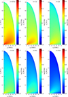 |
Fig. 1. Sectional views of the temperature evolution within the ejecta at t = 0.5 d, 1 d, 2 d, 4 d, 8 d, and 16 d following the WD–NS merger of our fiducial model. Here, vz and ve denote the ejecta velocities along the polar axis (θ = 0) and the equatorial plane (θ = π/2), respectively. The color scale indicates the logarithmic temperature. Owing to the 2D axisymmetry of the system in spherical coordinates, the temperature structure can be extended to the entire ejecta. |
Fig. 2 presents 2D sectional views of the photospheric evolution in velocity space for the fiducial model, as seen from different viewing angles. The central slices correspond to cross-sections through the center of the ejecta, with the line of sight fixed vertically downward. At early times (t ≲ 4 d), the observed photosphere lies near the outermost layer of the ejecta, regardless of the viewing angle. Due to the ellipsoidal velocity profile (Eq. (10)), the projected area of the observed photosphere naturally appears smaller for observers with lower values of θview. As the ejecta expands, the photosphere gradually recedes toward the ejecta’s inner layers. The morphology of the observed photosphere varies with the viewing angle. Compared to an on-axis observer (θview ≃ 0°), Fig. 2 shows that off-axis observers can probe deeper, more central regions of the ejecta.
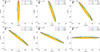 |
Fig. 2. Sectional views of the photosphere evolution in velocity space for our fiducial model, as seen by observers at different viewing angles. The line of sight is oriented vertically downward in each plane, and only the cross-section through the ejecta center is shown. Here, v∥ and v⊥ represent the velocity components parallel and perpendicular to the line of sight, respectively. Colored lines indicate the photospheric contours at various epochs following the WD–NS merger. |
5. Viewing-angle-dependent spectra and light curves
To construct the light curves, it is convenient to perform interpolation and integration by directly projecting the entire photosphere onto the mesh grid plane (see Sect. 4)13. Accordingly, the flux at an observed frequency νobs can be expressed as
 (24)
(24)
where h is the Planck constant, DL is the luminosity distance to the source, and kB is the Boltzmann constant. Defining the normalized wind velocity as  , the Doppler factor is given by
  , where Δθ is the angle between the velocity vector of the photosphere and the line of sight. The quantity dσij represents the infinitesimal projected photospheric surface element on the mesh grid. Flux densities per unit frequency and per unit wavelength are related via Fν|dν|=Fλ|dλ|, which yields
![Mathematical equation: $$ \begin{aligned} F_{\lambda }\left(\lambda _{\mathrm{obs} }\right)&\simeq \frac{2}{h^{4} c^{3} D_{\mathrm{L} }^{2}} \int \int _{S} \frac{\mathcal{D} ^{3}(h c / \mathcal{D} \lambda _{\mathrm{obs} })^{5}}{\exp \left(h c / \mathcal{D} k_{\mathrm{B} } \lambda _{\mathrm{obs} } T_{\text{ phot}}^{i j}\right)-1} d \sigma ^{i j}\nonumber \\&= \frac{2 h c^{2}}{ D_{\mathrm{L} }^{2}} \int \int _{S} \frac{ 1 / \mathcal{D} ^{2} \lambda _{\mathrm{obs} }^{5}}{\left[\exp \left(h c / \mathcal{D} k_{\mathrm{B} } \lambda _{\mathrm{obs} } T_{\text{ phot}}^{i j}\right)-1 \right]} d \sigma ^{i j} . \end{aligned} $$](/articles/aa/full_html/2026/02/aa56971-25/aa56971-25-eq44.gif) (25)
(25)
Using the calculated flux density Fν, one can derive the monochromatic AB magnitude using the standard definition Mν = −2.5log10(Fν/3631 Jy). For all subsequent calculations, we adopt a luminosity distance of DL = 10 pc, so that the resulting magnitudes correspond to absolute magnitudes. Magnitudes at other distances can be easily rescaled.
Figure 3 shows the temporal evolution of the emergent spectra from the WD–NS ejecta of the fiducial model at various viewing angles. Regardless of the viewing angle, the peak emission initially lies in the ultraviolet regime for t ≲ 4 d, and gradually shifts to the optical and subsequently to the infrared bands over time. The photospheric blackbody temperature can be estimated from Wien’s law, i.e., TBB = b/λmax, where b ≃ 0.29 cm K is the Wien’s displacement constant and λmax is the wavelength corresponding to the peak radiation intensity. As shown in Fig. 3, both the spectral intensity and the photospheric blackbody temperature exhibit significant viewing-angle dependence. For on-axis observers,  cools from ≃4.2 × 10⁴ K at t = 0.5 d to ≃3 × 10³ K at t = 25 d; whereas for equatorial observers, it decreases from ≃8.6 × 10⁴ K to ≃4 × 10³ K over the same time interval. Observers located at larger viewing angles receive substantially higher flux densities–up to nearly two orders of magnitude higher at early times. This enhancement arises from the emergence of more centrally located, and therefore hotter, photospheric layers at larger viewing angles, as well as from the increased projected photospheric area, as discussed in Sect. 4.
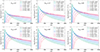 |
Fig. 3. Emergent spectra of WD–NS mSNe for θview = 0°, 15°, 30°, 45°, 60°, and 90°. Colored lines show the total observed emergent spectra at different epochs following the WD–NS merger of our fiducial model, assuming a luminosity distance of DL = 10 pc. The derived photospheric blackbody temperatures, |

To further illustrate the viewing-angle dependence of the multiband emission following a WD–NS merger in our fiducial model, we present ugriz-band14 light curves for different viewing angles in Fig. 4. We find that the peak absolute magnitudes in the optical bands span from ≃ − 12 mag for an on-axis view (θview ≃ 0°) to ≃ − 16 mag for an off-axis view (θview ≃ 90°). These optical peak luminosities are comparable to those of kilonovae arising from BNS and NS–BH mergers (see e.g., Nakar 2020; Kawaguchi et al. 2020b; Metzger 2020), although WD–NS thermal transients typically exhibit longer timescales to peak, usually ≳3–10 d. Since these WD–NS merger transients are powered solely by 56Ni heating, we introduce the term “mini-supernovae” (mSNe) to describe their thermal emission. Using the time-dependent emergent spectra obtained for WD–NS mSNe, we derive the luminosity light curves via  , where Fν is given by Eq. (24). The left panel of Fig. 5 presents the optical (g- and r-band) luminosity evolution of WD–NS mSNe for different viewing angles within our fiducial model (i.e., fej = 0.3 and fNi = 0.01). The WD–NS merger can power mSNe with peak luminosities in the range ≃1040–1042 erg s−1, depending on the viewing geometry. The peak timescale typically falls within 3–10 d. The observed directions θview ≃ 0° and θview ≃ 90° correspond to extreme, relatively rare cases. Most events are expected to be viewed at intermediate angles, yielding typical peak optical luminosities of ≃1041 erg s−1 and peak timescales of 3–10 d.
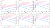 |
Fig. 4. Viewing-angle-dependent ugriz light curves of WD–NS mSNe for the fiducial model. Six angles are considered: θview = 0° (top left), 15° (top center), 30° (top right), 45° (bottom left), 60° (bottom center), and 90° (bottom right). |
We also investigated an alternative parameter set with fej = 0.03 and fNi = 0.001, corresponding to an ejecta mass of Mej = 0.03 M⊙ and a 56Ni mass of MNi = 0.001 M⊙, both an order of magnitude lower than those adopted in the fiducial model. This case is more relevant to stellar-mass BH-WD or He WD–NS mergers, which share similar ejecta properties but typically produce smaller ejecta and 56Ni masses (e.g., Metzger 2012; Fernandez & Metzger 2013; Margalit & Metzger 2016; Zenati et al. 2019; Fernández et al. 2019; Bobrick et al. 2022). The resulting optical light curves are shown in the right panel of Fig. 5 for different lines of sight. We find that the WD–NS mSNe with ejecta and 56Ni masses reduced by an order of magnitude relative to the fiducial model are expected to be fainter, with peak luminosities of ≃1039–1041 erg s−1 and shorter peak timescales of 2–5 d.
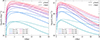 |
Fig. 5. Optical luminosity light curve of WD–NS mSNe. The left panel shows our fiducial model, assuming an ejecta mass of Mej = 0.3 M⊙ and a 56Ni mass of MNi = 0.01 M⊙. The right panel presents the WD–NS mSNe model in which both the ejecta and 56Ni masses are reduced by an order of magnitude, adopting Mej = 0.03 M⊙ and MNi = 0.001 M⊙. Different colors indicate different viewing angles at θview = 0°, 15°, 30°, 45°, 60°, and 90°. Solid and dashed lines correspond to the g- and r-band luminosities, respectively. |
6. Discussion
In comparison, our results are in good agreement with previous studies of WD–NS transients. For example, using 1D steady-state accretion-disk models for WD–NS mergers, Metzger (2012) suggested that a large fraction (≳50%) of the WD mass can be unbound as ejecta, while simultaneously synthesizing the 56Ni masses of 10−3–10−2 M⊙ within the ejecta. Treating the unbound ejecta as a single homologous shell and neglecting angular distributions, Metzger (2012) predicted optical transients with week-long peak timescales and peak luminosities of ≃1039–1041.5 erg s−1, following the semi-analytical model of Kulkarni (2005). Using 56Ni and ejecta velocity distributions from numerical simulations of CO and ONe WD accretion disks, and neglecting angular corrections, Fernández et al. (2019) showed that WD–NS merger transients can reach peak luminosities of ≃1040–1041 erg s−1 with week-long peak timescales, as inferred by Arnett’s semi-analytical model (Arnett 1979). Zenati et al. (2020) performed 3D hydrodynamic (SPH) and 2D hydrodynamic-thermonuclear (FLASH) simulations to study the disruption of CO WDs by NSs. They subsequently post-processed their simulations with a large nuclear reaction network and applied the SuperNu radiative-transfer code, assuming homologous ejecta expansion, to predict the observational signatures and detailed properties of CO WD–NS merger transients. Their models produced faint, red transients with peak luminosities around 1041 erg s−1 and peak timescales ranging from weeks to months, while neglecting viewing-angle dependence. Using a 1D analytic advection-dominated accretion-disk model, Kaltenborn et al. (2023) systematically investigated the inflow and outflow structure of WD–NS post-merger disks, including the effects of nuclear burning, neutrino emission, and wind ejection. They also simulated multiband light curves powered by radioactive iron-group elements using the SuperNu radiation-transfer code, predicting optical transients peaking at ≃1041–1042 erg s−1 with peak timescales of 5–8 d. More recently, Liu et al. (2025) employed detailed nucleosynthesis calculations with SkyNet in spherically symmetric ejecta models for WD–NS mergers, predicting optical transients with peak luminosities of a few 1041 erg s−1 and peak timescales of 2–4 d. Overall, while our results broadly agree with previous studies in terms of peak luminosities and timescales, our work uniquely highlights the previously unexplored viewing-angle dependence of WD–NS merger transients.
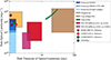 |
Fig. 6. Comparisons of the peak timescale and peak optical luminosity for various optical transients with t ≳ 1 d. The three blue-shaded regions, from dark to light, correspond to kilonova models associated with SMNS, HMNS or NS–BH, and prompt-collapse scenarios, respectively (Kawaguchi et al. 2020b). The yellow-shaded region indicates the parameter space for central-engine-powered kilonovae (i.e., the so-called “mergernova” model; Yu et al. 2013; Ai et al. 2025). The brown and green shaded regions denote core-collapse and type Ia SNe, respectively (Kasliwal 2012; Cenko 2017; Inserra 2019). The red and pink shaded regions represent the WD–NS mSNe explored in this work, corresponding to models with fiducial and reduced values of fej and fNi, respectively. For reference, we also indicate three well-known kilonova events associated with SGRB 170817A (red star; Villar et al. 2017), LGRB 211211A (orange diamond; Yang et al. 2022), and LGRB 230307A (green circle Levan et al. 2024), as well as the candidate WD–NS merger event AT2018kzr (purple cross; McBrien et al. 2019). |
We next explored how our WD–NS mSNe fit within the broader landscape of various optical transients in terms of their peak optical luminosities and timescales. Figure 6 compares different kilonova scenarios, including those from the BNS and NS–BH mergers, to illustrate where WD–NS mSNe lie in terms of their peak luminosities and timescales. Among these, Kawaguchi et al. (2020b) investigated the post-merger evolution and typical ejecta properties for both the BNS and the NS–BH binaries15. For BNS systems in particular, they considered different types of merger remnants, including a long-lived supermassive NS (SMNS), a hypermassive NS (HMNS), and a promptly collapsed BH. These models predict that the BNS and NS–BH kilonovae peak significantly earlier than the WD–NS counterparts presented in this work. Additionally, if a millisecond magnetar survives the BNS merger and injects extra energy into the ejecta (see e.g., Yu et al. 2013; Metzger & Piro 2014; Ai et al. 2025), the resulting kilonova light curve can become both brighter and longer-lived than that of a standard BNS kilonova. In contrast to typical kilonovae from BNS or NS–BH mergers, our WD–NS mSNe occupy the lower-right region of the parameter space, indicating that they are comparatively dimmer and peak significantly later. When adopting reduced values of fej and fNi, the region occupied by WD–NS mSNe shifts slightly toward the lower-left, indicating somewhat fainter and more rapidly evolving events than those with our fiducial fej and fNi values.
Figure 6 also highlights three well-known kilonova events associated with SGRB 170817A (Villar et al. 2017), LGRB 211211A (Yang et al. 2022), and LGRB 230307A (Levan et al. 2024), all of which are consistent with BNS or NS–BH merger scenarios and are difficult to reconcile with our 56Ni-powered WD–NS mSNe. Notably, if the WD–NS system contains a massive WD near the Chandrasekhar mass limit, the NS may merge into the center of the WD and trigger its collapse, potentially forming a millisecond magnetar as the central engine (Yang et al. 2022; Cheong et al. 2025; Zhang 2025). Alternatively, several recent studies suggest that, in WD–NS mergers, the NS may be spun up by accreting disrupted WD material, while its magnetic field can be amplified via dynamo processes, ultimately leaving behind a millisecond magnetar remnant (see e.g., Zhong & Dai 2020; Kaltenborn et al. 2023; Zhong et al. 2023, 2024a; Wang et al. 2024). Collectively, these studies offer valuable insight into the possible formation of a magnetar central engine and the corresponding central-engine-powered optical transients following WD–NS mergers, in which the ejecta can be accelerated and heated by magnetar spin-down, producing emission with shorter peak timescales and higher peak luminosities than those of our 56Ni-powered WD–NS mSNe. As shown in Fig. 6, the kilonovae associated with merger-origin LGRBs (i.e., LGRB 211211A and LGRB 230307A), may still arise from WD–NS mergers, but this would require the formation of a millisecond magnetar to act as the central engine to power them. Similar modeling that assumes a WD–NS merger origin with a magnetar remnant can also account for other fast-evolving optical transients, such as AT2018kzr (see Fig. 6; McBrien et al. 2019; Gillanders et al. 2020). We note that the ultimate fate of the merger remnant in WD–NS systems remains uncertain, and the probability of forming such magnetar-powered events in WD–NS mergers has yet to be conclusively determined. Since WD–NS mergers are generally not expected to produce significant amounts of r-process material, the spectroscopic identification of intermediate-mass elements (e.g., O, Mg, Si, and Ca) together with iron-peak elements in associated mSNe would strongly support a WD–NS merger origin (McBrien et al. 2019; Gillanders et al. 2020; Kaltenborn et al. 2023; Liu et al. 2025). Future discoveries of additional WD–NS merger candidates will provide valuable insight into their evolutionary pathways and remnant outcomes. On the theoretical side, more realistic models that incorporate detailed dynamical and thermodynamical evolution, as well as temperature- and wavelength-dependent opacities, are essential to fully understand these WD–NS transients, which we leave for future work.
7. Conclusions
Building on previous numerical simulations of WD–NS binaries undergoing unstable mass transfer, we adopted a semi-analytical discretization approach to investigate the viewing-angle dependence of thermal emission from such mergers. Using a 2D axisymmetric, polar-dominated wind ejecta model with heating from the radioactive decay of 56Ni, we tracked the evolution of the viewing-angle-dependent photosphere and its temperature. We find that for a WD–NS merger with a typical ejecta mass of Mej = 0.3 M⊙ and a 56Ni mass of MNi = 0.01 M⊙, the photosphere resides near the outermost ejecta layers for all viewing angles within ≲4 d after the merger, then recedes to deeper layers as the ejecta expands. The geometry of the observed photosphere varies with the viewing angle: off-axis observers see more centrally located, hotter ejecta regions than on-axis observers. Along the polar direction, the photospheric blackbody temperature cools from ≃4.2 × 10⁴ K to ≃3 × 10³ K between 0.5 d and 25 d, while along the equatorial direction it decreases from ≃8.6 × 10⁴ K to ≃4 × 10³ K over the same period. Our results show that the resulting emission intensity exhibits a strong viewing-angle dependence: larger viewing angles yield significantly higher fluxes owing to both a larger projected photospheric area and access to more centrally located (and hotter) ejecta layers. The peak absolute magnitudes in the optical bands range from ≃ − 12 mag for a polar line of sight to ≃ − 16 mag for an equatorial one, corresponding to peak optical luminosities of ≃1040–1042 erg s−1. Therefore, the peak optical luminosities of the thermal emission following WD–NS mergers are comparable to those of kilonovae from BNS and NS–BH mergers, although the WD–NS thermal transients generally evolve more slowly, with typical peak timescales of 3–10 d. Furthermore, lower ejecta masses and reduced 56Ni content naturally produce fainter transients with shorter peak timescales (see Fig. 6).
While our results are broadly consistent with earlier studies of WD–NS transients in terms of peak luminosities and peak timescales, our work uniquely emphasizes the viewing-angle dependence of WD–NS mSNe, which has not been systematically addressed previously. For kilonovae from BNS or NS–BH mergers, Kawaguchi et al. (2020b) showed that the observed flux is typically higher in the polar direction owing to the presence of multiple ejecta components, particularly the optically thick dynamical ejecta concentrated in the equatorial plane. In contrast, WD–NS mergers are expected to exhibit a fundamentally different ejecta morphology. As highlighted by Bobrick et al. (2022), only a small fraction of the WD debris (a few times 10−3 M⊙) is expected to be dynamically ejected and unbound. This ejecta undergoes negligible nuclear processing to synthesize 56Ni (Metzger 2012; Margalit & Metzger 2016; Fernández et al. 2019; Kaltenborn et al. 2023), resulting in a negligible observational impact. Our work can therefore motivate further investigations into the observational signatures and diversity of WD–NS merger transients. Moreover, given the rapid development in both ground-based and space-based GW astronomy, future multimessenger observations have the potential to provide further insights into WD–NS mergers (Yin et al. 2023; Kang et al. 2024; Morán-Fraile et al. 2024; Zhong et al. 2024b; Du et al. 2024; Yu et al. 2025), helping to constrain their properties and deepen our understanding of these systems.
Acknowledgments
We thank the anonymous referee for helpful comments. This work was supported by the National SKA Program of China (2020SKA0120300), the Beijing Natural Science Foundation (QY25099, 1242018), the National Natural Science Foundation of China (12573042), and the Max Planck Partner Group Program funded by the Max Planck Society. YK is supported by the China Scholarship Council (CSC).
References
- Abac, A. G., Abbott, R., Abouelfettouh, I., et al. 2024, ApJ, 970, L34 [CrossRef] [Google Scholar]
- Abbott, B. P., Abbott, R., Abbott, T. D., et al. 2017a, ApJ, 850, L39 [NASA ADS] [CrossRef] [Google Scholar]
- Abbott, B. P., Abbott, R., Abbott, T. D., et al. 2017b, ApJ, 848, L13 [CrossRef] [Google Scholar]
- Abbott, B. P., Abbott, R., Abbott, T. D., et al. 2017c, Phys. Rev. Lett., 119, 161101 [Google Scholar]
- Abbott, B. P., Abbott, R., Abbott, T. D., et al. 2017d, ApJ, 848, L12 [Google Scholar]
- Abbott, B. P., Abbott, R., Abbott, T. D., et al. 2018, Phys. Rev. Lett., 121, 161101 [Google Scholar]
- Abbott, B. P., Abbott, R., Abbott, T. D., et al. 2019, Phys. Rev. Lett., 123, 011102 [Google Scholar]
- Abbott, R., Abbott, T., Abraham, S., et al. 2021a, Phys. Rev. X, 11, 021053 [Google Scholar]
- Abbott, R., Abbott, T. D., Abraham, S., et al. 2021b, ApJ, 915, L5 [NASA ADS] [CrossRef] [Google Scholar]
- Abbott, R., Abbott, T. D., Acernese, F., et al. 2023a, Phys. Rev. X, 13, 041039 [Google Scholar]
- Abbott, R., Abbott, T. D., Acernese, F., et al. 2023b, Phys. Rev. X, 13, 011048 [NASA ADS] [Google Scholar]
- Ackley, K., Amati, L., Barbieri, C., et al. 2020, A&A, 643, A113 [NASA ADS] [CrossRef] [EDP Sciences] [Google Scholar]
- Ai, S., Gao, H., & Zhang, B. 2025, ApJ, 978, 52 [Google Scholar]
- Andreoni, I., Ackley, K., Cooke, J., et al. 2017, PASA, 34, e069 [NASA ADS] [CrossRef] [Google Scholar]
- Andreoni, I., Goldstein, D. A., Kasliwal, M. M., et al. 2020, ApJ, 890, 131 [NASA ADS] [CrossRef] [Google Scholar]
- Arcavi, I., Hosseinzadeh, G., Howell, D. A., et al. 2017, Nature, 551, 64 [NASA ADS] [CrossRef] [Google Scholar]
- Arnett, W. D. 1979, ApJ, 230, L37 [NASA ADS] [CrossRef] [Google Scholar]
- Arnett, D. 1996, Supernovae and Nucleosynthesis: An Investigation of the History of Matter, from the Big Bang to the Present (Princeton University Press) [Google Scholar]
- Arunachalam, P., Macias, P., & Foley, R. J. 2025, ArXiv e-prints [arXiv:2510.16121] [Google Scholar]
- Bian, L., Cai, R.-G., Cao, S., et al. 2021, Sci. China Phys. Mech. Astron., 64, 120401 [NASA ADS] [CrossRef] [Google Scholar]
- Bobrick, A., Davies, M. B., & Church, R. P. 2017, MNRAS, 467, 3556 [NASA ADS] [CrossRef] [Google Scholar]
- Bobrick, A., Zenati, Y., Perets, H. B., Davies, M. B., & Church, R. 2022, MNRAS, 510, 3758 [NASA ADS] [CrossRef] [Google Scholar]
- Cenko, S. B. 2017, Nat. Astron., 1, 0008 [Google Scholar]
- Chattopadhyay, T., Misra, R., Chattopadhyay, A. K., & Naskar, M. 2007, ApJ, 667, 1017 [NASA ADS] [CrossRef] [Google Scholar]
- Chatzopoulos, E., Wheeler, J. C., & Vinko, J. 2009, ApJ, 704, 1251 [Google Scholar]
- Chatzopoulos, E., Wheeler, J. C., & Vinko, J. 2012, ApJ, 746, 121 [Google Scholar]
- Chen, H.-L., Tauris, T. M., Chen, X., & Han, Z. 2022, ApJ, 930, 134 [Google Scholar]
- Chen, J., Shen, R.-F., Tan, W.-J., et al. 2024a, ApJ, 973, L33 [Google Scholar]
- Chen, M.-H., Li, L.-X., Chen, Q.-H., Hu, R.-C., & Liang, E.-W. 2024b, MNRAS, 529, 1154 [Google Scholar]
- Chen, J.-P., Shen, R.-F., & Chen, J.-H. 2025, ArXiv e-prints [arXiv:2510.27399] [Google Scholar]
- Cheong, P. C.-K., Pitik, T., Longo Micchi, L. F., & Radice, D. 2025, ApJ, 978, L38 [Google Scholar]
- Chornock, R., Berger, E., Kasen, D., et al. 2017, ApJ, 848, L19 [NASA ADS] [CrossRef] [Google Scholar]
- Chrimes, A. A., Gaspari, N., Levan, A. J., et al. 2025, A&A, 702, A168 [NASA ADS] [CrossRef] [EDP Sciences] [Google Scholar]
- Clocchiatti, A., & Wheeler, J. C. 1997, ApJ, 491, 375 [Google Scholar]
- Coulter, D. A., Foley, R. J., Kilpatrick, C. D., et al. 2017, Science, 358, 1556 [NASA ADS] [CrossRef] [Google Scholar]
- Cowperthwaite, P. S., Berger, E., Villar, V. A., et al. 2017, ApJ, 848, L17 [CrossRef] [Google Scholar]
- Díaz, M. C., Macri, L. M., Garcia Lambas, D., et al. 2017, ApJ, 848, L29 [Google Scholar]
- Drout, M. R., Piro, A. L., Shappee, B. J., et al. 2017, Science, 358, 1570 [NASA ADS] [CrossRef] [Google Scholar]
- Du, Z., Lü, H., Yuan, Y., Yang, X., & Liang, E. 2024, ApJ, 962, L27 [Google Scholar]
- Eggleton, P. P. 1983, ApJ, 268, 368 [Google Scholar]
- Eichler, D., Livio, M., Piran, T., & Schramm, D. N. 1989, Nature, 340, 126 [NASA ADS] [CrossRef] [Google Scholar]
- Evans, P. A., Cenko, S. B., Kennea, J. A., et al. 2017, Science, 358, 1565 [NASA ADS] [CrossRef] [Google Scholar]
- Fernandez, R., & Metzger, B. D. 2013, ApJ, 763, 108 [CrossRef] [Google Scholar]
- Fernández, R., Margalit, B., & Metzger, B. D. 2019, MNRAS, 488, 259 [CrossRef] [Google Scholar]
- Fragione, G. 2021, ApJ, 923, L2 [NASA ADS] [CrossRef] [Google Scholar]
- Gillanders, J. H., & Smartt, S. J. 2025, MNRAS, 538, 1663 [Google Scholar]
- Gillanders, J. H., Sim, S. A., & Smartt, S. J. 2020, MNRAS, 497, 246 [NASA ADS] [CrossRef] [Google Scholar]
- Goldstein, A., Veres, P., Burns, E., et al. 2017, ApJ, 848, L14 [CrossRef] [Google Scholar]
- Gomez, S., Hosseinzadeh, G., Cowperthwaite, P. S., et al. 2019, ApJ, 884, L55 [NASA ADS] [CrossRef] [Google Scholar]
- Han, M.-Z., Tang, S.-P., Hu, Y.-M., et al. 2020, ApJ, 891, L5 [CrossRef] [Google Scholar]
- Hu, L., Wu, X., Andreoni, I., et al. 2017, Sci. Bull., 62, 1433 [NASA ADS] [CrossRef] [Google Scholar]
- Inserra, C. 2019, Nat. Astron., 3, 697 [NASA ADS] [CrossRef] [Google Scholar]
- Kaltenborn, M. A., Fryer, C. L., Wollaeger, R. T., et al. 2023, ApJ, 956, 71 [NASA ADS] [CrossRef] [Google Scholar]
- Kang, Y., Liu, C., Zhu, J.-P., et al. 2024, MNRAS, 528, 5309 [Google Scholar]
- Kang, Y., Zhu, J.-P., Yang, Y.-H., et al. 2025, A&A, 698, A250 [NASA ADS] [CrossRef] [EDP Sciences] [Google Scholar]
- Kasen, D., Badnell, N. R., & Barnes, J. 2013, ApJ, 774, 25 [NASA ADS] [CrossRef] [Google Scholar]
- Kasliwal, M. M. 2012, PASA, 29, 482 [NASA ADS] [CrossRef] [Google Scholar]
- Kasliwal, M. M., Nakar, E., Singer, L. P., et al. 2017, Science, 358, 1559 [NASA ADS] [CrossRef] [Google Scholar]
- Kawaguchi, K., Kyutoku, K., Shibata, M., & Tanaka, M. 2016, ApJ, 825, 52 [NASA ADS] [CrossRef] [Google Scholar]
- Kawaguchi, K., Shibata, M., & Tanaka, M. 2020a, ApJ, 893, 153 [NASA ADS] [CrossRef] [Google Scholar]
- Kawaguchi, K., Shibata, M., & Tanaka, M. 2020b, ApJ, 889, 171 [NASA ADS] [CrossRef] [Google Scholar]
- Kilpatrick, C. D., Foley, R. J., Kasen, D., et al. 2017, Science, 358, 1583 [NASA ADS] [CrossRef] [Google Scholar]
- King, A., Olsson, E., & Davies, M. B. 2007, MNRAS, 374, L34 [NASA ADS] [Google Scholar]
- Kromer, M., & Sim, S. A. 2009, MNRAS, 398, 1809 [Google Scholar]
- Kulkarni, S. R. 2005, ArXiv e-prints [arXiv:astro-ph/0510256] [Google Scholar]
- Kyutoku, K., Ioka, K., Okawa, H., Shibata, M., & Taniguchi, K. 2015, Phys. Rev. D, 92, 044028 [NASA ADS] [CrossRef] [Google Scholar]
- Kyutoku, K., Fujibayashi, S., Hayashi, K., et al. 2020, ApJ, 890, L4 [Google Scholar]
- Levan, A. J., Gompertz, B. P., Salafia, O. S., et al. 2024, Nature, 626, 737 [NASA ADS] [CrossRef] [Google Scholar]
- Li, L.-X., & Paczynski, B. 1998, ApJ, 507, L59 [NASA ADS] [CrossRef] [Google Scholar]
- Lipunov, V. M., Gorbovskoy, E., Kornilov, V. G., et al. 2017, ApJ, 850, L1 [NASA ADS] [CrossRef] [Google Scholar]
- Liu, X.-X., Lü, H.-J., Chen, Q.-H., Du, Z.-W., & Liang, E.-W. 2025, ApJ, 988, L46 [Google Scholar]
- Maccary, R., Guidorzi, C., Maistrello, M., et al. 2026, J. High Energy Astrophys., 49, 100456 [Google Scholar]
- MacFadyen, A., & Woosley, S. E. 1999, ApJ, 524, 262 [NASA ADS] [CrossRef] [Google Scholar]
- Magee, M. R., Gillanders, J. H., Maguire, K., Sim, S. A., & Callan, F. P. 2021, MNRAS, 509, 3580 [Google Scholar]
- Manchester, R. N., Hobbs, G. B., Teoh, A., & Hobbs, M. 2005, AJ, 129, 1993 [Google Scholar]
- Margalit, B., & Metzger, B. D. 2016, MNRAS, 461, 1154 [Google Scholar]
- Margalit, B., & Metzger, B. D. 2017, MNRAS, 465, 2790 [Google Scholar]
- Margutti, R., & Chornock, R. 2021, ARA&A, 59, 155 [NASA ADS] [CrossRef] [Google Scholar]
- McBrien, O. R., Smartt, S. J., Chen, T.-W., et al. 2019, ApJ, 885, L23 [NASA ADS] [CrossRef] [Google Scholar]
- McCully, C., Hiramatsu, D., Howell, D. A., et al. 2017, ApJ, 848, L32 [NASA ADS] [CrossRef] [Google Scholar]
- Metzger, B. D. 2012, MNRAS, 419, 827 [CrossRef] [Google Scholar]
- Metzger, B. D. 2020, Liv. Rev. Relativ., 23, 1 [NASA ADS] [CrossRef] [Google Scholar]
- Metzger, B. D., & Piro, A. L. 2014, MNRAS, 439, 3916 [NASA ADS] [CrossRef] [Google Scholar]
- Metzger, B. D., Martinez-Pinedo, G., Darbha, S., et al. 2010, MNRAS, 406, 2650 [NASA ADS] [CrossRef] [Google Scholar]
- Morán-Fraile, J., Röpke, F. K., Pakmor, R., et al. 2024, A&A, 681, A41 [NASA ADS] [CrossRef] [EDP Sciences] [Google Scholar]
- Nadyozhin, D. K. 1994, ApJS, 92, 527 [Google Scholar]
- Nagy, A. P. 2018, ApJ, 862, 143 [Google Scholar]
- Nakar, E. 2020, Phys. Rep., 886, 1 [NASA ADS] [CrossRef] [Google Scholar]
- Narayan, R., Paczynski, B., & Piran, T. 1992, ApJ, 395, L83 [NASA ADS] [CrossRef] [Google Scholar]
- Nelemans, G., Yungelson, L. R., & Portegies Zwart, S. F. 2001, A&A, 375, 890 [NASA ADS] [CrossRef] [EDP Sciences] [Google Scholar]
- Nicholl, M., & Andreoni, I. 2025, Phil. Trans. Roy. Soc. Lond. A, 383, 20240126 [Google Scholar]
- Nicholl, M., Guillochon, J., & Berger, E. 2017a, ApJ, 850, 55 [NASA ADS] [CrossRef] [Google Scholar]
- Nicholl, M., Berger, E., Kasen, D., et al. 2017b, ApJ, 848, L18 [NASA ADS] [CrossRef] [Google Scholar]
- Paczynski, B. 1986, ApJ, 308, L43 [NASA ADS] [CrossRef] [Google Scholar]
- Paczynski, B. 1991, Acta Astron., 41, 257 [NASA ADS] [Google Scholar]
- Paczynski, B. 1998, ApJ, 494, L45 [Google Scholar]
- Paschalidis, V., MacLeod, M., Baumgarte, T. W., & Shapiro, S. L. 2009, Phys. Rev. D, 80, 024006 [Google Scholar]
- Paschalidis, V., Liu, Y. T., Etienne, Z., & Shapiro, S. L. 2011, Phys. Rev. D, 84, 104032 [NASA ADS] [CrossRef] [Google Scholar]
- Peng, Z.-K., Liu, Z.-K., Zhang, B.-B., & Gao, H. 2024, ApJ, 967, 156 [Google Scholar]
- Pian, E., D’Avanzo, P., Benetti, S., et al. 2017, Nature, 551, 67 [Google Scholar]
- Pinto, P. A., & Eastman, R. G. 2000, ApJ, 530, 757 [NASA ADS] [CrossRef] [Google Scholar]
- Pozanenko, A., Barkov, M. V., Minaev, P. Y., et al. 2018, ApJ, 852, L30 [NASA ADS] [CrossRef] [Google Scholar]
- Radice, D., Bernuzzi, S., & Perego, A. 2020, Ann. Rev. Nucl. Part. Sci., 70, 95 [NASA ADS] [CrossRef] [Google Scholar]
- Rastinejad, J. C., Gompertz, B. P., Levan, A. J., et al. 2022, Nature, 612, 223 [NASA ADS] [CrossRef] [Google Scholar]
- Rybicki, G. B., & Lightman, A. P. 1979, Radiative Processes in Astrophysics [Google Scholar]
- Sathyaprakash, B., Buonanno, A., Lehner, L., et al. 2019, Bull. Amer. Astron. Soc., 51, 251 [Google Scholar]
- Savchenko, V., Ferrigno, C., Kuulkers, E., et al. 2017, ApJ, 848, L15 [NASA ADS] [CrossRef] [Google Scholar]
- Shao, L., & Yagi, K. 2022, Sci. Bull., 67, 1946 [Google Scholar]
- Shao, L., Sennett, N., Buonanno, A., Kramer, M., & Wex, N. 2017, Phys. Rev. X, 7, 041025 [Google Scholar]
- Shappee, B. J., Simon, J. D., Drout, M. R., et al. 2017, Science, 358, 1574 [NASA ADS] [CrossRef] [Google Scholar]
- Smartt, S. J., Chen, T.-W., Jerkstrand, A., et al. 2017, Nature, 551, 75 [Google Scholar]
- Soares-Santos, M., Holz, D. E., Annis, J., et al. 2017, ApJ, 848, L16 [CrossRef] [Google Scholar]
- Tan, W.-J., Wang, C.-W., Zhang, P., et al. 2025, ApJ, 993, 89 [Google Scholar]
- Tanaka, M., & Hotokezaka, K. 2013, ApJ, 775, 113 [NASA ADS] [CrossRef] [Google Scholar]
- Tanaka, M., Kato, D., Gaigalas, G., & Kawaguchi, K. 2020, MNRAS, 496, 1369 [NASA ADS] [CrossRef] [Google Scholar]
- Tanvir, N. R., Levan, A. J., González-Fernández, C., et al. 2017, ApJ, 848, L27 [CrossRef] [Google Scholar]
- Toonen, S., Perets, H. B., Igoshev, A. P., Michaely, E., & Zenati, Y. 2018, A&A, 619, A53 [NASA ADS] [CrossRef] [EDP Sciences] [Google Scholar]
- Troja, E., Piro, L., van Eerten, H., et al. 2017, Nature, 551, 71 [NASA ADS] [CrossRef] [Google Scholar]
- Troja, E., Fryer, C. L., O’Connor, B., et al. 2022, Nature, 612, 228 [NASA ADS] [CrossRef] [Google Scholar]
- Utsumi, Y., Tanaka, M., Tominaga, N., et al. 2017, PASJ, 69, 101 [CrossRef] [Google Scholar]
- Valenti, S., Sand, D. J., Yang, S., et al. 2017, ApJ, 848, L24 [CrossRef] [Google Scholar]
- Verbunt, F., & Rappaport, S. 1988, ApJ, 332, 193 [NASA ADS] [CrossRef] [Google Scholar]
- Villar, V. A., Guillochon, J., Berger, E., et al. 2017, ApJ, 851, L21 [Google Scholar]
- Wang, S. Q., Wang, L. J., Dai, Z. G., & Wu, X. F. 2015, ApJ, 799, 107 [NASA ADS] [CrossRef] [Google Scholar]
- Wang, X. I., Yu, Y.-W., Ren, J., et al. 2024, ApJ, 964, L9 [Google Scholar]
- Wang, C.-W., Tan, W. J., Xiong, S. L., et al. 2025a, ApJ, 979, 73 [Google Scholar]
- Wang, P. F., Han, J. L., Yang, Z. L., et al. 2025b, Res. Astron. Astrophys., 25, 014003 [Google Scholar]
- Woosley, S. E. 1993, ApJ, 405, 273 [Google Scholar]
- Woosley, S. E., Eastman, R. G., & Schmidt, B. P. 1999, ApJ, 516, 788 [NASA ADS] [CrossRef] [Google Scholar]
- Xu, X.-T., Zhang, B.-B., Guo, Y.-L., & Li, X.-D. 2025, ApJ, 994, 264 [Google Scholar]
- Yang, J., Ai, S., Zhang, B.-B., et al. 2022, Nature, 612, 232 [NASA ADS] [CrossRef] [Google Scholar]
- Yang, Y.-H., Troja, E., O’Connor, B., et al. 2024, Nature, 626, 742 [NASA ADS] [CrossRef] [Google Scholar]
- Yin, Y.-H. I., Zhang, B.-B., Sun, H., et al. 2023, ApJ, 954, L17 [Google Scholar]
- Yu, Y.-W., Zhang, B., & Gao, H. 2013, ApJ, 776, L40 [CrossRef] [Google Scholar]
- Yu, S., Lu, Y., Jeffery, C. S., et al. 2025, ArXiv e-prints [arXiv:2511.20970] [Google Scholar]
- Yuan, F., & Zhang, B. 2012, ApJ, 757, 56 [Google Scholar]
- Zenati, Y., Perets, H. B., & Toonen, S. 2019, MNRAS, 486, 1805 [NASA ADS] [CrossRef] [Google Scholar]
- Zenati, Y., Bobrick, A., & Perets, H. B. 2020, MNRAS, 493, 3956 [NASA ADS] [CrossRef] [Google Scholar]
- Zhang, B. 2018, The Physics of Gamma-Ray Bursts (Cambridge: Cambridge University Press) [Google Scholar]
- Zhang, B. 2025, J. High Energy Astrophys., 45, 325 [Google Scholar]
- Zhang, B. B., Zhang, B., Sun, H., et al. 2018, Nat. Commun., 9, 447 [NASA ADS] [CrossRef] [Google Scholar]
- Zhao, J., Shao, L., Cao, Z., & Ma, B.-Q. 2019, Phys. Rev. D, 100, 064034 [Google Scholar]
- Zhong, S.-Q., & Dai, Z.-G. 2020, ApJ, 893, 9 [NASA ADS] [CrossRef] [Google Scholar]
- Zhong, S.-Q., Li, L., & Dai, Z.-G. 2023, ApJ, 947, L21 [NASA ADS] [CrossRef] [Google Scholar]
- Zhong, S.-Q., Li, L., Xiao, D., et al. 2024a, ApJ, 963, L26 [Google Scholar]
- Zhong, S.-Q., Meng, Y.-Z., & Gu, J.-H. 2024b, Phys. Rev. D, 110, 083001 [Google Scholar]
- Zhu, S.-Y., & Tam, P.-H. T. 2024, ApJ, 976, 62 [Google Scholar]
- Zhu, J.-P., Yang, Y.-P., Liu, L.-D., et al. 2020, ApJ, 897, 20 [NASA ADS] [CrossRef] [Google Scholar]
- Zhu, J.-P., Wu, S., Yang, Y.-P., et al. 2021a, ApJ, 917, 24 [NASA ADS] [CrossRef] [Google Scholar]
- Zhu, J.-P., Wu, S., Yang, Y.-P., et al. 2021b, ApJ, 921, 156 [NASA ADS] [CrossRef] [Google Scholar]
- Zhu, J.-P., Hu, R.-C., Kang, Y., et al. 2024, ApJ, 974, 211 [NASA ADS] [CrossRef] [Google Scholar]
- Zhu, J.-P., Zheng, J.-H., & Zhang, B. 2025a, MNRAS, 139, L149 [Google Scholar]
- Zhu, S.-Y., Deng, H.-Y., Zhang, F.-W., Mo, Q.-Z., & Tam, P.-H. T. 2025b, MNRAS, 541, 3236 [Google Scholar]
For comparison, the observed type Ia SN rate is approximately 4000 Myr−1 per MW-like galaxy (Toonen et al. 2018). Based on GW observations reported in GWTC-3, the local BNS merger rate is estimated to be in the range of [1, 30] Myr−1 per MW-like galaxy (Abbott et al. 2023b).
The existence of relativistic jets and associated high-energy emission in WD–NS mergers still remains uncertain and debated in the literature.
Most simulations excise the central engine region by imposing an inner boundary.
Bobrick et al. (2017) argues that winds from the accretion stream can further destabilize the system, yielding a much lower critical value qcrit ≃ 0.20, which is consistent with results by Kaltenborn et al. (2023).
Systems with different internal compositions can exhibit different ejecta properties, e.g., ONe WD–NS mergers are expected to eject more mass and yield higher 56Ni than CO WD–NS mergers (Fernández et al. 2019; Bobrick et al. 2022).
The main characteristics of wind dynamics and distribution in Fernández et al. (2019) are consistent with those reported in several other studies, including Fernandez & Metzger (2013), Zenati et al. (2019), Morán-Fraile et al. (2024).
For simplicity, we adopt a gray-opacity approximation to describe the overall thermal evolution and light curve morphology of the WD–NS merger ejecta. Nevertheless, frequency-dependent line opacities, as explored in various radiative-transfer studies of SNe and kilonovae, can alter the detailed spectral features and colors, especially through UV line blanketing by species such as C and O at late times (Pinto & Eastman 2000; Kasen et al. 2013; Tanaka et al. 2020; Magee et al. 2021). A detailed investigation of these effects in WD–NS thermal transients is beyond the scope of this work and should be addressed in future studies.
The Eddington approximation assumes local thermodynamic equilibrium (LTE). In the expanding ejecta of WD–NS mergers, LTE gradually breaks down as the optical depth decreases to τ ≲ 1, typically after ∼30 d for our fiducial ejecta parameters. Beyond this epoch, non-LTE effects, such as deviations from blackbody spectra and nonthermal excitation, are expected to become important (see e.g., Pinto & Eastman 2000; Kromer & Sim 2009; Tanaka & Hotokezaka 2013).
Readers seeking more details can refer to Appendix B of Zhu et al. (2020).
In the local coordinate system of the ejecta, we define a vector p pointing from  to the intersection point. Its direction determines the sign of p: p < 0 if p points along the line of sight, and p > 0 otherwise.
As described in Sect. 2, we consider cos θ ∈ [0, 1].
This approach is well justified when the angular extent of the WD–NS merger is effectively unresolved for an observer at a cosmological distance.
Details of the Sloan filter system can be found at https://www.sdss4.org
Because of limitations in temperature calculations, the peak brightness in Kawaguchi et al. (2020b) corresponds to the brightest point at t ≳ 1 d. We adopted the same convention in Fig. 6, noting that the BNS and NS–BH mergers may produce even brighter emission at earlier times, particularly in the ultraviolet band.
All Figures
|
Fig. 1. Sectional views of the temperature evolution within the ejecta at t = 0.5 d, 1 d, 2 d, 4 d, 8 d, and 16 d following the WD–NS merger of our fiducial model. Here, vz and ve denote the ejecta velocities along the polar axis (θ = 0) and the equatorial plane (θ = π/2), respectively. The color scale indicates the logarithmic temperature. Owing to the 2D axisymmetry of the system in spherical coordinates, the temperature structure can be extended to the entire ejecta. |
| In the text | |
|
Fig. 2. Sectional views of the photosphere evolution in velocity space for our fiducial model, as seen by observers at different viewing angles. The line of sight is oriented vertically downward in each plane, and only the cross-section through the ejecta center is shown. Here, v∥ and v⊥ represent the velocity components parallel and perpendicular to the line of sight, respectively. Colored lines indicate the photospheric contours at various epochs following the WD–NS merger. |
| In the text | |
|
Fig. 3. Emergent spectra of WD–NS mSNe for θview = 0°, 15°, 30°, 45°, 60°, and 90°. Colored lines show the total observed emergent spectra at different epochs following the WD–NS merger of our fiducial model, assuming a luminosity distance of DL = 10 pc. The derived photospheric blackbody temperatures, |
| In the text | |
|
Fig. 4. Viewing-angle-dependent ugriz light curves of WD–NS mSNe for the fiducial model. Six angles are considered: θview = 0° (top left), 15° (top center), 30° (top right), 45° (bottom left), 60° (bottom center), and 90° (bottom right). |
| In the text | |
|
Fig. 5. Optical luminosity light curve of WD–NS mSNe. The left panel shows our fiducial model, assuming an ejecta mass of Mej = 0.3 M⊙ and a 56Ni mass of MNi = 0.01 M⊙. The right panel presents the WD–NS mSNe model in which both the ejecta and 56Ni masses are reduced by an order of magnitude, adopting Mej = 0.03 M⊙ and MNi = 0.001 M⊙. Different colors indicate different viewing angles at θview = 0°, 15°, 30°, 45°, 60°, and 90°. Solid and dashed lines correspond to the g- and r-band luminosities, respectively. |
| In the text | |
|
Fig. 6. Comparisons of the peak timescale and peak optical luminosity for various optical transients with t ≳ 1 d. The three blue-shaded regions, from dark to light, correspond to kilonova models associated with SMNS, HMNS or NS–BH, and prompt-collapse scenarios, respectively (Kawaguchi et al. 2020b). The yellow-shaded region indicates the parameter space for central-engine-powered kilonovae (i.e., the so-called “mergernova” model; Yu et al. 2013; Ai et al. 2025). The brown and green shaded regions denote core-collapse and type Ia SNe, respectively (Kasliwal 2012; Cenko 2017; Inserra 2019). The red and pink shaded regions represent the WD–NS mSNe explored in this work, corresponding to models with fiducial and reduced values of fej and fNi, respectively. For reference, we also indicate three well-known kilonova events associated with SGRB 170817A (red star; Villar et al. 2017), LGRB 211211A (orange diamond; Yang et al. 2022), and LGRB 230307A (green circle Levan et al. 2024), as well as the candidate WD–NS merger event AT2018kzr (purple cross; McBrien et al. 2019). |
| In the text | |
Current usage metrics show cumulative count of Article Views (full-text article views including HTML views, PDF and ePub downloads, according to the available data) and Abstracts Views on Vision4Press platform.
Data correspond to usage on the plateform after 2015. The current usage metrics is available 48-96 hours after online publication and is updated daily on week days.
Initial download of the metrics may take a while.