| Issue |
A&A
Volume 706, February 2026
|
|
|---|---|---|
| Article Number | A351 | |
| Number of page(s) | 18 | |
| Section | Astrophysical processes | |
| DOI | https://doi.org/10.1051/0004-6361/202556986 | |
| Published online | 23 February 2026 | |
Hillas meets Eddington: The case for blazars as ultra-high-energy neutrino sources
1
European Southern Observatory Karl-Schwarzschild-Straße 2 85748 Garching bei München, Germany
2
Excellence Cluster ORIGINS Boltzmannstr. 2 D-85748 Garching bei München, Germany
3
Max-Planck-Institut für Plasmaphysik Boltzmannstr. 2 DE-85748 Garching, Germany
4
Institute for Theoretical Physics, Heidelberg University Philosophenweg 12 69120 Heidelberg, Germany
★ Corresponding author: This email address is being protected from spambots. You need JavaScript enabled to view it.
Received:
25
August
2025
Accepted:
17
December
2025
Abstract
Context. Jetted active galactic nuclei aligned with our line of sight known as blazars are promising high-energy neutrino source candidates. However, leptohadronic models face challenges in describing neutrino emission within a viable energy budget and their predictive power are limited by the commonly used single-zone approximation and reliance on phenomenological parameters.
Aims. We tested the scenario where energetic protons are continuously accelerated up to ultra-high energies in inner blazar jets, while accounting for the source energetics and jet dynamics.
Methods. We present a new leptohadronic model, where a sub-Eddington jet evolves from being magnetically to kinetically dominated. A constant fraction of 10−6–10−8 of the electrons and protons picked up by the jet are continuously accelerated to a power-law spectrum. We can estimate their normalization and maximum energies based on the local magnetic field strength, turbulence, and medium density, for which we assumed power-law profiles. The model parameters are thus directly tied to the jet physics and are comparable in number to a single-zone model. We then calculate the emission along the jet, including neutrinos and electromagnetic cascades.
Results. Applying the model to IceCube candidate TXS 0506+056, we find that protons accelerated in the inner jet produce a neutrino flux up to ∼100 PeV that is consistent with the public IceCube ten-year point-source data. Proton emission at 0.1 pc describes the X-ray and γ-ray data, while electron emission at the parsec scale describes the optical data. Protons carry a power of about 1% of the Eddington luminosity. The particle spectra follow E−1.8, with diffusion scaling as E0.3, ruling out Bohm-like diffusion. Additional particle injection near the broad line region can reproduce the 2017 flare associated to a high-energy neutrino. We also applied the model to the blazar PKS 0605-085, which could be associated with a recent neutrino detected by KM3NeT above 100 PeV.
Conclusions. Magnetic acceleration in blazar jets can describe multimessenger observations with viable energetics. Our model constrains jet properties such as the energy-dependent particle diffusion and predicts the spatial distribution of the multiwavelength and neutrino emission along the jet. The results suggest that blazars are efficient neutrino emitters at ultra-high energies, making them prime candidates for future experiments targeting this challenging energy range.
Key words: astroparticle physics / neutrinos / radiation mechanisms: non-thermal / methods: numerical / galaxies: jets / quasars: general
© The Authors 2026
 Open Access article, published by EDP Sciences, under the terms of the Creative Commons Attribution License (https://creativecommons.org/licenses/by/4.0), which permits unrestricted use, distribution, and reproduction in any medium, provided the original work is properly cited.
This article is published in open access under the Subscribe to Open model. This email address is being protected from spambots. You need JavaScript enabled to view it. to support open access publication.
1. Introduction
The origin of the cosmic rays remains a subject of considerable debate in astroparticle physics. Over the past decade, the IceCube Neutrino Observatory at the South Pole has detected a cosmic flux of neutrinos extending to energies of at least 10 petaelectronvolt (PeV, IceCube Collaboration 2013; Aartsen et al. 2013, 2015a,b), triggering a debate on the cosmic accelerators responsible for these particles (e.g., Stecker et al. 1991; Halzen & Hooper 2002; Hooper 2016; Murase et al. 2020).
In the ultra-high-energy (UHE) regime, defined here as above ∼100 PeV, IceCube has so far only set upper limits on the diffuse neutrino flux (Abbasi et al. 2025). On the other hand, the KM3NeT observatory in the Mediterranean Sea has recently reported the detection of a > 100 PeV muon, likely produced by a neutrino of even higher energy (Aiello et al. 2025). Given that hadronic interactions typically transfer ∼5% of a proton’s energy into neutrinos, an UHE neutrino would then be expected to originate in an astrophysical source capable of accelerating protons or other nuclei to the exaelectronvolt (EeV) regime (i.e., an UHE cosmic-ray accelerator).
Current neutrino experiments face two challenges in the UHE range: (1) the detection of UHE neutrinos, owing to their low number fluxes; and (2) the identification of UHE neutrinos, owing to limited energy resolution in this energy regime. While problem (1) can only be circumvented with increased statistics and next-generation detectors targeting the UHEs, problem (2) can also potentially be addressed with existing data, by using astrophysics-driven predictions to interpret high-energy neutrino detections associated to known sources.
Among the most promising neutrino source candidates are blazars, namely, active galactic nuclei (AGNs) with a relativistic jet that is approximately aligned with our line of sight. Multiple blazars have been associated with IceCube events at different confidence levels (CLs; e.g., Padovani & Resconi 2014; IceCube Collaboration 2018; Giommi et al. 2020; Franckowiak et al. 2020; Sahakyan et al. 2022; Abbasi et al. 2022a). The UHE event detected by KM3NeT also seems to be spatially consistent with multiple blazars lying within the reconstructed spatial uncertainty (Adriani et al. 2025).
One of the best-studied IceCube candidates is blazar TXS 0506+056 (z ≃ 0.34 Paiano et al. 2018). The source is an intermediate-synchrotron-peaked BL Lac (IBL), which was later identified as a masquerading BL Lac (Padovani et al. 2019). In other words, it was found to belong to a class of flat-spectrum radio quasars (FSRQs) whose broad line and thermal emission is swamped by the jet emission. In 2017, IceCube detected a throughgoing muon event from the direction of TXS 0506+056 during a six-month-long state of enhanced GeV and TeV γ-ray emission (IceCube Collaboration 2018). The neutrino, originating from just below the IceCube horizon, produced a muon in the ice that eventually crossed the IceCube detector, depositing an energy of 23 TeV. The IceCube collaboration estimate a value of 45 TeV for the most likely muon energy as it entered the detector, implying that the neutrino should have a true energy exceeding ∼100 TeV. Since the neutrino interacted outside the detector, the emitted muon lost an unknown amount of energy before detection. The actual neutrino energy may therefore have been significantly higher and remains largely unconstrained beyond this lower limit.
The 2017 neutrino detection from TXS 0506+056 was followed by a series of theoretical papers describing the emission. Models in which protons reach only sub-PeV energies (emitting neutrinos with ∼100 TeV in the observer’s frame) generally face three challenges: (1) neutrino production by sub-PeV protons is inefficient in blazars, thus implying an extremely high power in relativistic protons, often orders of magnitude in excess of the Eddington limit (e.g., Keivani et al. 2018; Gao et al. 2019; Cerruti et al. 2019); (2) the hadronic interactions responsible for neutrino emission trigger electromagnetic cascades down to the X-ray regime and, thus, X-ray observations severely limit the extent of these interactions (e.g., see Fig. 3 of Gao et al. 2019); (3) synchrotron emission by sub-PeV protons is inefficient and, thus, the observed GeV γ-ray flare is typically described purely by inverse Compton emission by electrons, with a negligible contribution from protons (e.g., Rodrigues et al. 2021; Sahakyan et al. 2022). This makes this class of models difficult to test experimentally and weakens the causal connection between the 2017 neutrino detection and the simultaneous γ-ray flare, which was the main motivation for considering this blazar a strong neutrino source candidate.
In contrast, in single-zone models where protons reach EeV energies and radiate efficiently in highly magnetized jet regions, the observed γ-ray fluxes are dominated by proton synchrotron emission (e.g., Aharonian 2002). However, as we discuss later in this paper, even in this scenario the presence of external photon fields is essential for the z the emission from hadronic cascades peaks at higher frequencies, making a hadronic flare scenario more consistent with X-ray observations.
In this work, we test a leptohadronic blazar model in which protons and electrons are continuously picked up and magnetically accelerated in a sub-Eddington jet whose Poynting flux is gradually converted into kinetic flux. We numerically simulate the emitted multiwavelength and neutrino fluxes. Applying the model to TXS 0506+056, we show that protons can reach EeV energies in the inner (sub-pc scale) jet, producing a flux of ∼100 PeV neutrinos compatible with the IceCube point-source limits without violating the jet energetics. Meanwhile, the optical emission is shown to be dominated by the parsec-scale jet, from synchrotron emission by the co-accelerated electrons. We also apply the model to source PKS 0605-085, one of the blazars possibly associated to the 2024 UHE event detected by KM3NeT. Our results show that some AGN jets are likely UHE neutrino sources and provide new constraints on the likely mechanisms of particle acceleration and diffusion in relativistic jets.
The paper is organized as follows. In Section 2, we introduce our model of a magnetically launched blazar jet whose properties evolve continuously. We show that protons can be accelerated to EeV energies outside the BLR. We also argue that multimessenger data can help constrain particle diffusion and acceleration. In Section 3, we describe how we applied the model to IceCube candidate source TXS 0506+056, showing that UHE protons can aptly describe the time-averaged γ-ray emission through proton synchrotron, as well as the point source IceCube flux, with a sub-Eddington jet power. The model can also describe the multiwavelength flare coincident with a high-energy IceCube event in 2017, by considering a temporary increase in the injected particle number in the vicinity of the BLR. In Section 4, we apply the model to blazar PKS 0605-085, located within the uncertainty region of an UHE neutrino recently detected by the KM3NeT experiment. In Section 5, we discuss the results and we suggest how the model can eventually be expanded and tested with time-domain observations. We summarize our conclusions in Section 6.
2. Model description
We expanded1 the single-zone approach to blazar modeling by implementing an extended jet model where the physical parameters vary continuously and the jet power is limited to sub-Eddington levels. The model is governed by parameters describing the radial profile of the magnetic field strength and turbulence level, the environmental matter density, and the particle diffusion coefficient. From those results, we were able to self-consistently derive the jet dynamics, as well as the maximum energy of the protons and electrons, assuming stochastic Fermi-type particle acceleration in the turbulent magnetic field. We then calculated the multiwavelength and neutrino emission along the jet using a time- and energy-dependent numerical framework. By fitting the model to multimessenger data, we indirectly constrained the underlying jet parameters.
2.1. Jet dynamics
We assumed the jet to be symmetric in the polar direction and, thus, we modeled all dynamic properties as a function of the radial coordinate, r, or the distance to the supermassive black hole. The profile of the jet cross-section depends on the evolution of the jet bulk Lorentz factor. At a given distance, r, the maximum opening of the jet is dictated by the relativistic beaming effect: θj(r)≤1/Γj(r), where θj is the jet’s half-opening angle, and Γj is the bulk Lorentz factor. For the sake of generality, we considered the possibility that the jet is further collimated (either by structured toroidal magnetic fields in the magnetized regime or by external ram pressure). For convenience, we parametrized this effect by a constant factor fθ < 1, such that θj(r) = fθ/Γj(r). Assuming the jet has a circular cross-section with radius, Rj, this results in Rj = rtan(fθ/Γj)≈rfθ/Γj for fθΓj ≪ 1. We leave more complex jet collimation and velocity profiles (see e.g., Zhang & Giannios 2021; Lucchini et al. 2022) for future studies.
We parametrized the jet power as a fraction of the Eddington luminosity, Lj/LEdd < 1, where LEdd = 1.26 × 1046(MBH/108 M⊙) erg/s. We treated this ratio as a model parameter. For simplicity, we assumed energy conservation along the jet, expressed as
 (1)
(1)
where  is the Poynting power and Lk = πRj′2uT′2Γj(Γj − 1)βc is the kinetic jet power2. The energy density of thermal (cold) protons, uT′(r) = mpc2n′T(r), is a function of the local density of the ambient medium and the local flow speed, as we describe later in this paper.
In Eq. (1), the power deposited in nonthermal protons and electrons, Le + Lp, and their associated radiation, Lrad, is neglected, as we limit these contributions to only a fraction of the jet power,
 (2)
(2)
This ensures that the jet does not dissipate away its power in the form of nonthermal particles. The relation Le(r)≪Lp(r) follows from the fact that, as we show in Sect. 3, protons reach ∼EeV energies in this model in the inner jet, while the electrons typically do not surpass tens of GeV along the entire jet. The relation Lrad(r)≪Lp(r) was derived from the fact that the environment is optically thin, even for protons at the highest energies. As described later in this section, the values of Lp, e(r) were estimated self-consistently based on the local jet parameters and the particle number density available in the medium, while Lrad(r) is derived from the additional radiation modeling.
We next model the evolution of the magnetic field strength. If the jet is magnetically launched, at the jet base, we approximately have Γj ≈ 1 and LB ≈ Lj, and thus  . We can then model the radial profile of the magnetic field strength as a power law of r as
 (3)
(3)
We fixed the jet base to rbase = 3 rS, where rS = 2GMBH/c2 is the Schwarzschild radius, calculated for each source based on the estimated mass of the supermassive black hole (SMBH). We treated αB as a free model parameter in the range αB ≳ 1, leading to a gradual reduction in the Poynting flux. As an example, we consider a source with MBH = 6 × 10⁸ M⊙ and, therefore, rbase ∼ 1015 cm and LEdd = 8 × 1046 erg s−1. For Lj = 0.5 LEdd and a collimation factor fθ = 0.2, Eq. (3) implies a magnetic field at the jet base of B′∼104 G. If the jet is launched via a Blandford-Znajek mechanism, such field strengths are achievable at sub-Eddington accretion rate (e.g., Katsoulakos & Rieger 2018), as supported by GRMHD simulations of magnetically arrested discs (e.g., Tchekhovskoy et al. 2011; McKinney et al. 2012). In the same example, assuming a magnetic field evolution index of αB = 1.1, we obtained B′ = 70 G at r = 1017 cm, which is approximately the BLR scale. Field strengths of 10 < B′/G < 100 at these scales are characteristic of proton synchrotron frameworks (Cerruti et al. 2015). In our model, strong magnetic fields near the BLR are energetically viable (cf. Liodakis & Petropoulou 2020) owing to the high degree of collimation of the jet, as in all three sources we test, we obtained a best-fit value of fθ ≈ 0.2. By considering instead a noncollimated scenario with fθ ≲ 1, Eq. (3) would instead yield B′∼1 G around the BLR scale, which typically leads to a scenario where inverse Compton scattering dominates the γ-ray emission (see Petropoulou et al. 2015; Cerruti et al. 2019; Gao et al. 2019; Sahakyan et al. 2022, for a direct comparison). Finally, at the parsec scale, the magnetic field strength in our example lies at the ∼G level, which is compatible with radio observations of parsec-scale blazar cores and core-shift measurements (Lobanov 1998; Savolainen et al. 2008; O’Sullivan & Gabuzda 2009). More complex magnetic field parameterizations, potentially constrained by source measurements (cf. e.g. Ro et al. 2023), are conceivable and left for future study.
The acceleration of the jet and the evolution of jet’s bulk Lorentz factor is expected to be related to the MHD framework (Tchekhovskoy et al. 2009; Pu & Takahashi 2020). In our model, the evolution of the jet’s bulk Lorentz factor emerges from the combination of the Poynting power profile (as discussed above) and the flux of cold (thermal) protons, ṄT, carried by the jet,
 (4)
(4)
To estimate the thermal proton flux, we assume that the density of the surrounding medium follows a power-law profile n(r)∼r−αn. We normalize n(r) by considering the line-of-sight hydrogen column density: NH = ∫RBLRkpcn(r)dr = 1022ξH cm−2, where the dimensionless parameter ξH represents the hydrogen column density in units of 1022 cm−2. Values of 10−2 ≲ ξH ≲ a few are consistent with the low obscuration levels typically observed in blazars (Eitan & Behar 2013; Willingale et al. 2013). The flux of locally entrained protons in the comoving jet frame is thus  . Once entrained, particles are also advected downstream, leading to an additional flux
  . The total rate of thermal particles in the flow,
  , is well approximated by
 (5)
(5)
Any value of αn < 2αB leads to a decrease in the magnetization, σ = B′2/(4π nTmpc2), along the jet, as the Poynting power is converted into kinetic power:
 (6)
(6)
Thus, the magnetization is unity at about the scale of the BLR radius, at which point the jet transitions from magnetically to kinetically dominated, which is consistent with simulations of magnetically driven jets (e.g., Komissarov et al. 2007). The maximum Lorentz factor is given by the initial magnetization,
 (7)
(7)
Intrinsic Doppler factors in the range of 10–40 have been inferred in the parsec-scale jets of numerous blazars based on variability and VLBI observations (e.g., Jorstad et al. 2017) and are supported at r ≲ 103rS by GRMHD simulations of magnetically launched jets (Tchekhovskoy et al. 2009; Pu & Takahashi 2020). We impose αn < 2 to ensure that the jet reaches Γmax below the 10 pc scale and subsequently decelerates, as suggested by observations (Ros et al. 2020), rather than approaching Γmax asymptotically. Heating or various instabilities developing along the jet can lead to further deceleration at large scales (Laing & Bridle 2014; Homan et al. 2015; Perucho 2019). Because the model is only sensitive to the inner jet dynamics, we kept the energy conservation assumption for the sake of simplicity.
Finally, we derived the number of relativistic (nonthermal) protons and electrons. We assumed that a constant fraction fNT of the thermal particles picked up by the jet are accelerated to a nonthermal power-law distribution. The flux of nonthermal protons and electrons is then given by
 (8)
(8)
 (9)
(9)
where ṄT is given by Eq. (5) and fe ≥ 1 is the number of electrons per proton. In a Poynting-dominated scenario, the jet may be pair-dominated, implying a ratio  > 1, assuming charge neutrality. In reality, as the jet becomes less radiation-dominated, the presence of pairs should decrease, implying a nonconstant profile of fe(r). However, owing to limited data; here, we treat the pair-to-proton fraction fe ≥ 1 as a constant model parameter and leave more sophisticated treatments for future work.
2.2. How multimessengers constrain particle acceleration
We go on to discuss the maximum energies of the nonthermal electrons and protons undergoing continuous Fermi-type particle acceleration along the jet. We consider an energy-dependent particle mean free path motivated by quasilinear theory, which results in a spatial diffusion coefficient of the form  c, where
  is the Larmor radius of the relativistic particle,
  the coherence length of the underlying turbulence spectrum, and η = (δB/B)2 < 1 the ratio of turbulent to total magnetic energy. Motivated by simulations in which turbulence and magnetic reconnection peak near shocks or recollimation zones and decline downstream (Komissarov et al. 2007; Inoue et al. 2011); Tchekhovskoy:2015yih; (Duran et al. 2017; Martí et al. 2016; Baring et al. 2017), we assume a power-law profile of η at the large scales: η ∝ r−αη (αη > 0) for r ≫ RBLR, treating αη as a free parameter to be constrained by the model fit. At r ≪ RBLR, the turbulence level is poorly constrained; however, it is clear that the bulk of the high-energy emission should not originate from very deep in the BLR, since this would lead to strong attenuation via γγ-annihilation (e.g. Poutanen & Stern 2010; Boettcher & Els 2016) and to abundant cascade emission in the X-ray and γ-ray bands, are limited by observations (Reimer et al. 2019; Rodrigues et al. 2019; Oikonomou et al. 2019). We thus implement an exponential cutoff in the turbulence level below a given value of rη, max ≈ 1–3 RBLR. The full form of our turbulence profile is then (see also Inoue et al. 2011):
![Mathematical equation: $$ \begin{aligned} \eta \,(r) = \eta _{\mathrm{max} }\,\frac{ \exp \left(-\dfrac{r_{\eta ,\mathrm{max} }}{r} \right) \left( \dfrac{r}{r_{\eta ,\mathrm{max} }} \right)^{-\alpha _\eta } }{ \mathrm{max} \left[ \exp \left(-\dfrac{r_{\eta ,\mathrm{max} }}{r} \right) \left( \dfrac{r}{r_{\eta ,\mathrm{max} }} \right)^{-\alpha _\eta } \right] }\cdot \end{aligned} $$](/articles/aa/full_html/2026/02/aa56986-25/aa56986-25-eq19.gif) (10)
(10)
We treated the maximum acceleration efficiency and its position (ηmax and rη, max), as well as the index αη, as model parameters. While ηmax and rη, max are mainly responsible for the energy and location of the UHE proton acceleration in the inner jet, αη, is responsible for the maximum energy of the emitting electrons at and above the parsec scale.
We began by considering particle acceleration at mildly relativistic shocks via the first-order Fermi process (diffusive shock acceleration, DSA), a widely adopted framework for modeling the nonthermal emission from localized jet regions (e.g., Marscher & Gear 1985; Kirk et al. 1998; Zech & Lemoine 2021). Neglecting the effects of oblique shocks, this first-order process is expected to lead to power-law spectra with p ≳ 2 (e.g., Sironi & Spitkovsky 2011; Marcowith et al. 2016; Crumley et al. 2019). Assuming the coherence length to be limited by the jet diameter,  , the resulting acceleration timescale is approximately given by c tacc′DSA = (1/η)(c/Vs)2R′j(R′L/R′j)δ, where Vs is the shock speed. In the so-called Bohm limit, δ = 1, we retrieved c tacc′DSA, Bohm = (1/η)(c/Vs)2RL′.
Alternatively, if particles are accelerated stochastically in the turbulent magnetic field along the jet, classical second-order Fermi processes (e.g., Jokipii 1966; Skilling 1975; Duffy & Blundell 2005; Katarzyński et al. 2006; Strong et al. 2007) yield an acceleration timescale approximately given by  , where
  is the Alfvén speed. In the absence of feedback (Lemoine et al. 2024), second-order Fermi acceleration may result in particle spectra harder than produced by DSA, 1 < p < 2 (e.g., Virtanen & Vainio 2005; Rieger et al. 2007); at the same time, we can see that the efficiency of this process differs from DSA by a factor (Vs/VA)2. In our inner jet model, this is therefore a viable dominant process of continuous re-acceleration in regions of high magnetization, where VA ∼ c. We note that in the case of strong turbulence, a modified description may be necessary (e.g., Lemoine 2022). On the other hand, in the kinetically dominated regime of the jet, DSA or shear-type particle acceleration may become dominant and lead to further particle energization (e.g., Wang et al. 2024a,b). We leave the connection between our inner jet model and potential large-scale jet DSA or shear acceleration for future work.
Next, we explored the potential of multimessenger data to constrain the turbulence characteristics influencing acceleration and diffusion, namely, η and δ, in the simple formalism introduced above. We started with neutrino observations. As shown by Rodrigues et al. (2024b), the integrated ten-year IceCube point source flux can be constrained under the assumption of a model-dependent source signal spectrum. Because most of the signal-like events consist of throughgoing muons that were produced outside the instrumented volume, it is challenging to estimate their true energy, and we can only produce a band of energy-dependent flux limits. However, neutrino emission in blazar jets is most efficient in the UHE range, where the protons have sufficient energy to interact with both optical broad lines and infrared thermal emission from the dusty torus (Murase et al. 2014, see Appendix A). In the sub-PeV range, the source is optically thin to photopion interactions; thus, producing a high neutrino flux requires a super-Eddington power in relativistic protons (e.g., Gao et al. 2019; Keivani et al. 2018, see Appendix A for a more in-depth discussion). This raises the question of the conditions under which protons might be accelerated to hundreds of PeV within a magnetized jet model (see Petropoulou et al. 2022, for an in-depth discussion). The jet is optically thin to photohadronic interactions and to proton synchrotron emission, as t′syn ∼ 100Rj′(fθ/0.2)−1(E′p/EeV)−1(B/30 G)−2 at r = 3RBLR. Proton acceleration is therefore limited only by diffusive escape. Assuming again that  , protons escape diffusively on a timescale approximately given by c tesc′=R′j (R′j/R′L)δ. Equating this escape timescale with the timescale of acceleration, we obtain
  for DSA, while
  for stochastic acceleration.
As an example, we can assume a scenario where the turbulent fraction reaches its maximum at rη, max = 0.1 pc, with B = 30 G and ηmax = 0.3. We assume, for simplicity, Vs ≈ c (which is optimistic for DSA but conservative for stochastic acceleration). In the case of DSA in the Bohm limit (δ = 1), protons will achieve a maximum energy of
 (11)
(11)
For stochastic acceleration, assuming a Kolmogorov-type diffusion exponent of δ = 0.3, we have
 (12)
(12)
where the additional dependence on the particle density parameter αN is introduced by the Alfvén speed. This illustrates that under suitable conditions, protons can achieve energies of at least hundreds of PeV just outside the BLR for DSA at mildly relativistic shocks as well as by stochastic acceleration in magnetic turbulence, owing to the high magnetization (σ ≲ 1) of the inner jet at these scales.
To constrain the population of co-accelerated electrons, we turn to optical observations. Assuming that the bulk of the emitting electrons are in the fast-cooling regime, their maximum energy can be derived by equating acceleration with synchrotron cooling, t′syn = (9m3)/(4e4c3B′2γ′). At scales of r ∼ pc, this yields
 (13)
(13)
 (14)
(14)
We know that the observed synchrotron peak frequency of a typical IBL, νsynpeak ∼ 1015 Hz, must be produced by electrons with characteristic energy,  . This indicates that a stochastic acceleration scenario with a mild (Kolmogorov-type) energy-dependence of the diffusion coefficient (Eq. (14)) is more appropriate for describing the observed IBL synchrotron emission while also allowing for UHE proton acceleration, as described above.
This point is illustrated in Fig. 1. In the upper panel, we show a DSA scenario in the Bohm limit (δ = 1), and in the lower panel a second-order Fermi acceleration scenario with Kolmogorov-type energy-dependence of the diffusion coefficient (δ = 0.3). In blue, we show the expected acceleration timescales; in shades of red, the timescales of electron-synchrotron energy loss (which limits the acceleration of electrons) and diffusive escape (which limits the acceleration of protons). The timescales were calculated for a large range of parameter values (1 < B′/G < 50 and 10−3 < η < 0.1) to account for the fact that protons and electrons may interact at different locations along the jet. The green band on the left side shows the range of maximum electron energies necessary to describe the typical IBL synchrotron peak frequency. The green band on the right side shows the range of maximum proton energy that allows for sufficient neutrino emission with sub-Eddington energetics (cf. Appendix A). We show as black crosses the maximum electron and proton energies predicted by the model along the jet, following Eqs. (11)–(14). By comparing how the crosses intersect with the green bands, we can see how a stochastic acceleration scenario with a diffusion exponent δ = 0.3 can produce the electron and proton energies necessary to describe the multimessenger data, while diffusion in the Bohm limit yields maximum electron energies that would lead to synchrotron emission in the X-ray range, which excludes this scenario in this source class. A scenario where the optical emission originates in cooled TeV electrons is also excluded, since the resulting spectrum would be too soft to describe data from our target sources. Alternatively, in a scenario with an extremely weak turbulent magnetic field (η ∼ 10−7), electrons would have the necessary GeV energies (Eq. (13)), but protons would achieve only ∼100 TeV (Eq. (11), see Fig. 12 by Podlesnyi & Oikonomou 2025). This would result in a sub-PeV leptohadronic model and thus require a super-Eddington proton power (cf. Fig. A.1). Based on our requirement of sub-Eddington jet energetics, we exclude Bohm-like diffusion in our inner jet model. We assume δ = 0.3 throughout the rest of this work.
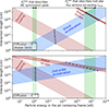 |
Fig. 1. Two scenarios of diffusion and acceleration. Upper panel: Diffusive shock acceleration with a diffusion coefficient D′E ∼ E′ − 1. Lower panel: Stochastic acceleration with D′E ∼ E′0.3. The timescales are given for the wide range of parameters η, B′, and R′j expected at distances 1017 cm ≲ r ≲ pc, as detailed in the main text. Black crosses show the maximum energy of electrons and protons predicted by the respective scenario. Green bands show the allowed range of E′e and E′p necessary to describe the multimessenger data. |
In addition, we want to discuss the number and spectral index of the relativistic particles. As we show in Section 3, fitting the model to data will favor a scenario where turbulence peaks at scales of rη, max ∼ 0.1 pc, where the local magnetization is just below unity, σ ≲ 1. Stochastic acceleration may then lead to particle distributions with spectral index in the range 1 ≲ p ≲ 2, depending on particle escape and possible feedback between the relativistic particles and the turbulence. In this work, we adopted a fiducial value of pe, p = 1.8, reflecting conditions where feedback plays a non-negligible role (Lemoine 2022). As the results will show, this spectral index can describe data with a reasonable electron-to-proton number ratio 1 ≲ fe ≲ 10. Values of p ≲ 1.7 would reduce the total number of protons necessary to describe high-energy data, leading to electron-to-proton ratios in excess of 100, while p ≳ 1.9 would require more protons than electrons, a challenging scenario under charge neutrality. For p > 2.0, the contribution from low-energy protons would make the total required proton power approach the Eddington limit, making an UHE model energetically unfeasible.
We fixed the minimum Lorentz factor of both protons and electrons to γe′min = γp′min = 100. While cold particles do not directly contribute to the emission, this choice still impacts the total number of nonthermal protons and electrons. The power in nonthermal particles is dominated by the relativistic protons with maximum Lorentz factor, which can reach  in the inner jet, as we have shown. Integrating the proton distribution and enforcing Lp < 0.1Lj, we obtain a rough constraint on the maximum ratio between nonthermal and thermal protons,
 (15)
(15)
Considerably higher values of the steady-state nonthermal-to-thermal particle number ratio would imply a quick dissipation of the jet’s energy into UHE protons.
2.3. Nonthermal emission
We numerically calculated the steady-state photon and neutrino fluxes emitted by the nonthermal electrons and protons in 30 zones per decade in r, uniformly distributed in log(r). A higher number would not affect the results (since the total fluxes are scaled down for consistency, cf. Appendix C), nor the number of model parameters (since in each zone the local jet parameters are given by the continuous functions discussed above). At each discrete location, we consider a spherical zone and calculate the radiative processes using the AM3 code (Klinger et al. 2024)3, which numerically solves the coupled energy- and time-dependent differential equations governing the evolution of all relevant particle species (see details in Appendix C). We do not explicitly model acceleration from the thermal pool; instead, we continuously inject nonthermal protons and electrons with a power-law spectrum estimated as described previously, based on the local jet parameters. The cooling and emission processes are time-dependent and their evolution is nonlinear, and include all channels of pair production and the subsequently triggered nonlinear cascades. In each zone, we evolve the continuity equations up to the steady state; we then compare the total jet emission to multimessenger data, thus indirectly constraining the underlying jet parameters. In Appendix C, we further detail the implementation of the radiation model and the treatment of the external photon fields from the BLR and the dusty torus.
3. Application to IceCube candidate TXS 0506+056
Next, we show how the model can describe the multimessenger emission from the blazar TXS 0506+056, starting with the steady-state emission. To optimize the model parameters, we calculated the reduced chi-squared value between the predicted fluxes and the multiwavelength data (listed in Table 1), following the binning procedure described in Appendix C and further detailed in Rodrigues et al. (2024b), and performed a minimization using MINUIT (James & Roos 1975). We note that the data being fitted are nonsimultaneous; we therefore do not condition the best fit on a limit on the best-fit χ2 value, which includes the intrinsic source variability. We also treat data below 100 GHz as upper limits, since these fluxes are likely to have additional contributions from the large-scale jet.
Best-fit parametersand core assumptions of the extended jet model.
Figure 2a shows the total predicted steady-state multiwavelength and neutrino spectra resulting from particle interactions along the extended jet. Figure 2b refers to the 2017 flaring event. The blue, red, and purple curves represent the individual contributions from the sampled stationary emission zones along the jet: the blue curves represent photon emission from primary relativistic electrons, red from relativistic protons, and purple the muon neutrinos at Earth resulting from photohadronic interactions (see Appendix C for details on the model implementation), which is the all-flavor neutrino spectrum divided by three. The total photon and neutrino spectra are shown as black curves, representing the integrated emission along the extension of the jet. As we can see, this scenario, where turbulent magnetic fields in the inner jet accelerate protons to UHEs leads to the γ-ray fluxes being dominated by proton emission. As detailed in Appendix C, the peak of the GeV γ-ray flux is dominated by proton synchrotron emission, while at lower and higher frequencies there are additional contributions from pairs emitted in Bethe-Heitler and photomeson interactions. The optical flux is dominated by synchrotron emission from primary electrons, and the X-ray spectrum has contributions from both electron and hadronic emission. The predicted neutrino energy flux peaks at  and is compatible with the 68% CL IceCube point source flux limits derived from the public 10 year dataset (green band). We refer to Appendix A, where we discuss the neutrino emission in greater depth.
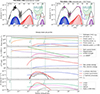 |
Fig. 2. Extended jet model applied to the IceCube candidate blazar TXS 0506+056, fitted to the average multiwavelength emission (panel a, data taken from Rodrigues et al. 2024b, see references therein) and during the 2017 flaring event (panel b, data in magenta taken from IceCube Collaboration 2018; Keivani et al. 2018). The top panels show the best-fit spectra. The color curves show the photon emission by primary electrons (blue), photon emission by protons (red), and muon neutrino emission (purple) from the successive zones along the jet. The dashed curves in panel b show the emission from the flare zone. The black curves show the total emission. The green band shows the 68% CL limits on the neutrino point source flux from the source (Rodrigues et al. 2024b), and the dark red curve the UHE sensitivity of IceCube-Gen2 (Aartsen et al. 2021). The pink curve shows the BLR and accretion disk continuum emission, and the bright green curve the host galaxy contribution (see Rodrigues et al. 2024b). In panels c–g, we show the evolution along the extended jet of the jet energetics (c), dynamics (d), particle profile (e) and emission (f, g). |
To better understand how the extended jet contributes to the emission, we show in Figs. 2c–g the best-fit evolution with r of key quantities relating to the energetics, dynamics, particle acceleration, and emission. In Fig. 2c, we can see how the Poynting flux (green) converts into kinetic flux under the energy conservation assumption. Just outside the BLR, the physical power deposited in nonthermal protons (red curve, given by Lp = Lp′Γj2/2) reaches the maximum value of a few percent of the jet luminosity and then decreases again with r as the magnetic field becomes again less turbulent, gradually weakening proton acceleration.
In Fig. 2d, we show in green the evolution of the jet magnetization. At about 0.02 pc, or at the edge of the BLR, the magnetization (shown in purple) has dropped to σ ∼ 1, and the jet becomes matter-dominated, as discussed Section 2.1 (Eq. (6)). In the range where stochastic acceleration is most efficient, around rη, max ≈ 0.1 pc (see pink curve), the magnetic field is of the order of a few tens of gauss (green curve), as is usual in proton synchrotron models (cf. Section 5 and references therein). The jet, which is nonrelativistic at the base (Γj = 1), has been accelerated to a maximum Lorentz factor of Γj ≈ 40 at the parsec scale, before slowing down due to the matter density evolving with αn = 1.95 < 2. Beyond the 10 pc scale, the jet dynamics is not constrained by the model (see below), and energy losses to the environment may decelerate the jet faster than predicted here.
In Fig. 2e we show the evolution of the maximum energy of protons (red) and electrons (blue). Protons achieve their maximum energy of ∼EeV just outside the BLR, which results directly from the best-fit value of the maximum-turbulence scale, rη, max. As both the magnetic field strength and the turbulent fraction decrease, so does the maximum proton energy, and by 10 pc protons reach a maximum energy of about 1 PeV. On the contrary, the maximum energy of electrons is independent of the magnetic field strength, since this regulates both synchrotron cooling and acceleration. This results in an approximately constant maximum electron energy of about 10 GeV (blue curve, cf. black crosses in Fig. 1). This constant energy, which comes from the assumption that diffusion scales with E0.3, is responsible for the predicted synchrotron emission peaking at 1014.5 Hz, in accordance with observations (Fig. 2).
Figure 2f shows the observed photon flux produced by electrons (blue) and protons (red) along the jet, integrated across frequencies. In other words, the blue curve shows the integral of each of the photon spectra emitted by primary electrons, shown in blue in Fig. 2, as a function of the position along the jet, and similarly for protons. Unsurprisingly, the proton synchrotron emission (dashed red curve) is brightest at the same length scale where protons achieve their maximum energy of about 1 EeV, at rp syn, max = 0.07 pc or about 3 rBLR. The emission of neutrinos (black curve) and hadronic photons (dotted red curve) reaches its maximum slightly later, at around rp syn, max = 0.2 pc. At this point, the number of accelerated protons has not changed significantly compared to rp syn, max, yet their energy is concentrated in a slightly lower range, up to a maximum energy of a few hundreds of PeV (cf. Fig. 2e). At this energy, protons interact resonantly with thermal photons from the peak of the thermal emission from the dusty torus: E′p ≈ 200 (40/Γj)(500 K/Ttorus) PeV. The emitted neutrinos have an energy of (1 + z)Eν = 400 (500 K/Ttorus) PeV, which is independent of the jet’s bulk Lorentz factor.
We can see that there is also a lower peak in the neutrino emission as the jet crosses the BLR. This is driven by interactions with broad line photons. In our best-fit model, the protons have only reached a maximum energy of 10 PeV by the time the jet crosses the BLR. This allows the resonant production of neutrinos with energy (1+z)Eν ≥ 1.5 (10.2 eV/EH I) PeV for the H Lyα line, and (1+z)Eν ≥ 370 (10.2 eV/EH II) TeV for the He II Lyα line, both of which are explicitly included. Importantly, the number of He II photons is a factor of eight lower than that of H I photons, and all BLR photons combined are a factor of ten less numerous than those emitted by the dust torus. This is the reason why UHE neutrino emission in broad-line blazars is more efficient than in the sub-PeV and PeV range. Because of this, the total neutrino energy flux emitted along the extended jet at and below the PeV range is a factor 50 less than that above the 100 PeV range (cf. A.1). As we have just shown, this general effect is relatively independent of the Lorentz bulk factor of the jet.
For electrons, the profile of the emitted luminosity behaves differently, as shown by the blue curve in Fig. 2f: starting from the onset of stochastic acceleration, their emitted synchrotron flux increases, driven by the increase in the Lorentz factor, up to the parsec scale, where it reaches its maximum. The emission then starts to decrease. This decrease is both intrinsic, owing to the decrease in the magnetic field strength and constant maximum electron energy, and additionally in the observer’s frame, owing to the deceleration of the jet and with it the decreasing relativistic boost of the emission.
Finally, in Fig. 2g we show the electromagnetic energy flux emitted along the jet by both protons and electrons, integrated in four frequency ranges: γ-rays (red), X-ray (magenta), optical (green), and radio (black). As we can see by comparison with Fig. 2f, the bulk of the observed γ-ray emission is dominated by proton synchrotron (see also Fig. C.1 in Appendix C). The X-ray emission has two components: one follows the hadronic cascades, with a first peak when the jet crosses the BLR and a higher one at 0.2 pc. But X-rays also have a sub-dominant contribution from electron emission, as we can see in the spectrum of Fig. 2, and thus the bulk of the jet’s X-ray emission extends out to the parsec scale. The optical emission is strongest between 0.1 and 10 pc, peaking at a few parsec, as it is dominated by the peak of the electron synchrotron emission. Beyond the parsec scale, as second-order Fermi acceleration becomes inefficient and electrons obtain gradually lower maximum energies, the synchrotron emission starts peaking at increasingly lower frequencies. We thus see the radio emission below 300 GHz (black curve) peaking at the parsec scale, and extending out to about 10 pc. As we can see from Fig. 2, this gradual decrease in the synchrotron peak frequency describes well the flat radio spectrum observed from the source down to about ∼100 GHz. Beyond this length scale, additional emission is expected from, for instance, shock or stochastic-shear processes, which are not included in the model.
Next, we extended the model to describe the 2017 γ-ray flare of TXS 0506+056, during which a high-energy neutrino was observed from the direction of the blazar. We tested the scenario where the number of accelerated particles is temporarily boosted in one of the segments of the jet:  . This could be due to a temporary increase in the density of particles available for acceleration, for example if a star crosses the jet perpendicularly (e.g., Bosch-Ramon et al. 2012; Araudo et al. 2013; Fichet de Clairfontaine et al. 2025). The flare is described by only two additional parameters: its location, r = rflare, and the number of particles injected there, fNTflare > fNT. The jet parameters at rflare are given by the same best-fit jet dynamics as in the steady state. For each value of rflare along the jet (discretized along our grid with 30 cells per decade, see Appendix C), we calculated the emitted photon and neutrino flux and add these fluxes to the steady-state jet emission. We then optimized the two parameters by minimizing the chi-squared fit to the multiwavelength fluxes observed during the flare.
We show the result in Fig. 2b. The steady-state emission is the same as in the baseline extended jet model of Fig. 2a; the photon and neutrino emission from the segment affected by the temporary additional particle injection are shown as dashed curves. The total flux enhancement at different wavelengths during the flare depends on its location. The best fit is rflare = 2.6 rBLR, or about 0.05 pc (see Table 1), so proton emission at this location is more efficient than that of electrons (cf. Fig. 2f). As a result, the γ-ray flux increases by a factor of two compared to the steady state, describing the simultaneous Fermi LAT and MAGIC observations (IceCube Collaboration 2018; Keivani et al. 2018), while the optical and X-ray fluxes increase by a factor of only 1.5, describing well the quasisimultaneous data. The X-ray spectrum has a contribution from both electron synchrotron and hadronic cascades (cf. Fig. C.1). The energy-integrated neutrino flux increases by a factor of 2.3 during the flare, with the peak energy increasing only marginally (cf. Fig. A.1)
This description of the 2017 flare requires the temporary acceleration of a fraction fNTflare = 8 × 10⁻⁶ of the thermalized particles (Table 1), corresponding to a local nonthermal particle flux of  . Approximating the local maximum proton energy to 1 EeV, this yields a total physical proton luminosity during the flare of Lp = 3 × 1046(Γj/30)2 erg/s, which represents 35% of the Eddington luminosity, or 80% of the jet power. This is a dramatic temporary increase in the power deposited in protons compared to the steady state (∼1% of the Eddington luminosity), but still below the total local jet power.
4. Application to KM3NeT candidate PKS 0605-085
In 2023, the KM3NeT neutrino observatory in the Mediterranean Sea detected a throughgoing muon event with  (Aiello et al. 2025), the highest confirmed energy of any cosmic neutrino detected to date. We apply our UHE extended jet model to the FSRQ PKS 0605-085 (4FGL J0608-0835, BZQ J0607-0834), one of the 50 brightest known radio blazars and one of the four γ-ray sources identified inside the 99% containment region of the KM3Net event (Adriani et al. 2025). Of the three other sources, only the BL Lac PMN J0616-1040 is also detected in radio, and the only one with a measured spectroscopic redshift (z = 0.87: Shaw et al. 2012). It is also the only source undergoing a year-long period of enhanced γ-ray activity during the detection.
Since in our model the γ-ray flux comes from proton synchrotron emission, a simultaneous enhancement of neutrinos and γ-rays can be naturally explained, as shown in Fig. 2 for TXS 0506+056. However, the model does not guarantee a correlation between γ-rays and neutrinos as a general feature, since neutrino production depends additionally on the local target photon density. Shaw et al. (2012) report a broad line luminosity of LHβ = 1043.7 erg/s and LMg II = 1044.3 erg/s. Using their estimates of the virial black hole mass from both lines and taking the weighted average, we obtain MBH = 108.87 ± 0.26 M⊙, yielding LEdd = 1046.97 ± 0.26 erg s−1. Adopting the average line flux reported by Vanden Berk et al. (2001), we can extrapolate the total BLR luminosity from LHβ and LMg II. A weighted mean between the two yields LBLR = 1045.26 ± 0.08 erg s−1. This implies a total bolometric disk luminosity of Ldisc ≈ 20LBLR = 1046.6 erg s−1 ≈ 0.4 LEdd. We report these values in Table 1. For the canonical radiative efficiency of 10%, the reference accretion power, and hence the maximum jet power, is Lacc ≃ 10LEdd. Starting from the best-fit parameters of the extended jet applied to TXS 0506+056, we performed a local optimization by minimizing the chi-squared value to multiwavelength data (see Rodrigues et al. 2024b, and references therein). Given the source’s low Galactic latitude bII = −13.5°, we correct the optical data for Galactic extinction (cf. similar procedure by Kivokurtseva & Troitsky (2025)): we adopt the H I column density from Bekhti et al. (2016), convert it to V-band extinction (Foight et al. 2016), and then derive the extinction for other bands, Aλ, following Schlafly & Finkbeiner (2011), Fitzpatrick (1999). The corrected flux is then F0 = Fobs 100.4Aλ. In Fig. 3 we show the data and the best-fit results. As in the case of TXS 0506+056, the γ-ray spectrum is dominated by proton emission. As we dissect in Appendix C (cf. middle panel of Fig. C.1), the peak of the γ-ray emission, at a few hundreds of MeV, is dominated by proton synchrotron. The γ-ray spectrum above 1 GeV, as well as the X-ray flux, are dominated by hadronic cascade emission. The fluxes from 100 GHz up to optical are described by electron synchrotron emission. The magnetic field turbulence decays with αη = 1.4, a steeper profile than for TXS 0506+056. This can describe well the source’s low synchrotron peak frequency (estimated following Glauch et al. 2022, see Table 1), as opposed to TXS 0506+056, which is an ISP blazar.
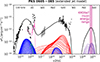 |
Fig. 3. Extended jet model applied to KM3NeT candidate blazar PKS 0605-085. Data adopted from Rodrigues et al. (2024a, see references therein). The curves are color coded as in Fig. 2. The magenta band shows the muon energy of the event KM-230213. |
The predicted neutrino emission peaks at 200 PeV. As shown by the magenta band in Fig. 3, the maximum neutrino energy predicted by the model is consistent with the energy range of the muon detected by KM3NeT. As detailed in the bottom panel of Fig. A.1, the 200 PeV neutrinos at the peak of the spectrum are produced in interactions between the UHE protons and the infrared emission from the dusty torus. The density of infrared photons is calculated based on the derived accretion disc luminosity, assuming a standard covering factor of 0.3, as specified in Table 1 and detailed further in Rodrigues et al. (2024b). We leave for future work a quantitative discussion on the necessary neutrino flux level to produce a single event in KM3NeT, since this would (a) require fitting the model to time-selected data around the neutrino detection, and (b) be subject to large uncertainties inherent to the Poissonian nature of the detection. However, it is clear that for a period of γ-ray flaring the model predicts an enhancement of the neutrino flux, as in the case of TXS 0506+056, owing to the fact that protons are responsible for both γ-ray and neutrino emission and the target thermal photons from the dusty torus are static.
5. Discussion
One of the defining features of this model is that the bulk of the observed γ-ray flux is predicted to be emitted by relativistic protons, co-accelerated by the same mechanism as the nonthermal electrons. This feature is shared with the classic proton blazar model (Mannheim 1995), and with works applying that model to TXS 0506+056 (Cerruti et al. 2019; Banik & Bhadra 2019) and other blazars (e.g., Muecke et al. 2003) in a single-zone framework. In that sense, this work embeds the single-zone proton synchrotron model into a broader framework that connects the predicted emission with the extended geometry and energetics of the jet. Our model also includes the broad line and thermal photon fields surrounding the jet. As explained in Appendix A, the presence of external photons is crucial for efficient neutrino emission, even in an UHE scenario.
The fact that the bulk of the γ-ray flux is emitted by protons means that the model establishes a direct causal connection between the 2017 γ-ray flare of TXS 0506+056 and the high-energy neutrino event detected simultaneously by IceCube. In contrast, leptohadronic models where the maximum proton energies are limited to the sub-PeV range (e.g. Gao et al. 2019; Keivani et al. 2018) predict protons to contribute negligibly to the γ-ray flux and only marginally to the X-ray flux, thus weakening the connection between the γ-ray flare and the associated neutrino emission.
The model suggests a high ratio between the neutrino and the γ-ray luminosity of hadronic blazar candidates. Defining Yγν = Lν/Lγ, where Lγ is the integrated luminosity between 0.1 and 100 GeV, the results imply a value of Yγν = 0.3 for TXS 0506+056 (0.7 for PKS 0605-085). Given that the 7 year UHE IceCube flux limits constrain Yνγ < 0.13 for blazars (Aartsen et al. 2016), and the 12.6 year limits (Fig. A.1) are even more constraining by a factor of 2.5 at 100 PeV (Abbasi et al. 2025), it is clear that TXS 0506+056 must be an exceptionally bright neutrino emitter compared to the average blazar of the same luminosity. This is compatible with the fact that the source stands out as the second hottest spot in the IceCube 10 year point-source sky (Aartsen et al. 2020). The green band in Fig. 2 represents the limits required to produce such a point source signal at the 68% CL, and the model is consistent with those constraints.
As we demonstrate in Fig. A.1 (Appendix A), blazars with low-power accretion discs are inefficient UHE neutrino candidates, as UHE neutrino emission depends crucially on the infrared photons from the dusty torus as targets (Murase et al. 2014; Rodrigues et al. 2018, 2024b). At the same time, the bulk of the γ-ray luminosity is relatively independent of the external photon fields, since it is dominated by proton synchrotron emission (cf. Fig. C.1). Conversely, in a scenario where proton acceleration begins inside the BLR, the resulting neutrino spectrum can be considerably softer, leading to a relative enhancement to the PeV neutrino flux (Murase et al. 2014). Ultimately, observational constraints such as spectroscopic data must be considered when modeling the jet emission (e.g. Padovani et al. 2022; Paiano et al. 2023; Rodrigues et al. 2024b), making an extrapolation to the blazar population a sensitive matter.
We now discuss the results related to the acceleration efficiency profile (Eq. (10)). The best-fit location of the maximum acceleration efficiency falls consistently in the range rη max ≳ RBLR (cf. Figs. 2d and C.2b). This is consistent both with γ-ray observations and with single-zone leptohadronic blazar models (Poutanen & Stern 2010; Oikonomou et al. 2021; Rodrigues et al. 2024a,b). In a scenario of continuous stochastic acceleration, this may reflect a change of the turbulence level within the jet, induced by its interaction with the environment around the inhomogeneous BLR edge (cf. Marscher et al. 1992; Mizuno et al. 2011; Marscher 2014; Perucho 2019).
Magnetic reconnection is also likely to play a significant role near the peak of our acceleration efficiency profile (Sironi & Spitkovsky 2014; Guo et al. 2015; Werner et al. 2018). In particular, it is possible that a site of reconnection around the r ∼ 0.01 pc scale injects energized particles into the larger-scale turbulence, which then continuously re-accelerates them to higher energies (Comisso et al. 2017; Comisso & Sironi 2018). A more in-depth analysis is necessary to eventually tease apart the contribution of these different processes in our target sources.
In the large-scale matter-dominated flow, shocks can also lead to efficient DSA (Eqs. (11) and (13)), which is typically sufficient to explain observations of hot spots of radio galaxies (Bell 1978; Blandford & Ostriker 1978). In addition, shear acceleration could become efficient, leading to further particle energization along the jet (Rieger 2019; Wang et al. 2024a; Rieger & Duffy 2025). An extension of the model to include these additional contributions could eventually help connecting the high-energy emission described here, with the observed radio flux below 100 GHz, which our model underestimates (Figs. 2a, 3). These processes could also lead to the acceleration of protons and other nuclei up to UHEs beyond the kiloparsec scale (e.g., Rachen & Biermann 1993; Wang et al. 2024b). Since the weak magnetic fields and low densities in the large-scale jet preclude a substantial contribution of high-energy photons or neutrinos to the overall source spectrum, we neglect the large-scale jet altogether in this study, and we suggest an extension of the model to the large-scale jet as an important follow-up study, with consequences for the broader population of jetted AGN as UHE cosmic-ray sources.
Regarding the composition of the relativistic particle population, the best-fit parameters suggest a ratio of electrons to protons of order fe ∼ 10. While this may in general suggest a pair-dominated jet, it is important to note that the emission from protons and electrons originates at different length scales, and we assume a constant fraction ξH of ambient particles picked up by the jet along these different scales. A stronger constraint on the chemical composition of the jet may therefore require a deeper analysis in the time domain supported perhaps by a more sophisticated modeling framework.
From Fig. 2f, we see that our model allows for some delay between the observed γ-ray and optical signals, but only of order (ropt/c)(1 + z)/(ΓjδD)≲1 (ropt/pc)(30/Γj) day. This is compatible with observations of γ-ray flares accompanied closely by optical flares (e.g., Cohen et al. 2014; Liodakis et al. 2019; Rajput et al. 2021; de Jaeger et al. 2023), given the typical uncertainties. A more promising avenue for testing the model on a source-by-source basis may be intra-day variability (Wagner & Witzel 1995; Gupta et al. 2008) near the peak frequency of the optical emission. Indeed, Δtopt < 1 (roptpeak/pc)(fθ/0.2)(Γj/30)−2 day suggests a more compact optical emission region, possibly attached to the peak of the turbulence profile.
6. Conclusion
We present a model of the extended inner blazar jet that can describe the multiwavelength emission of blazar TXS 0506+056 during the quiescent and the flaring state, as well as the point-source IceCube flux limits, while maintaining consistency with the source energetics. Rather than parameterizing the nonthermal populations of electrons and protons, we derived their properties assuming a continuous profile of the magnetic field, turbulence, and particle density. Because of the dependence of the model on the jet dynamics, the model is able to capture the extended nature of the jet with a number of free parameters comparable to a typical single-zone model.
The jet is magnetically launched close to the supermassive black hole. In our best-fit scenario, the jet carries 45% of the Eddington luminosity and the B-field strength scales as B′∝r−1.06, leading to the gradual acceleration of the jet. At the 0.1 pc scale, the jet achieves a bulk Lorentz factor of 30 and its magnetization has dropped below unity. At these scales, a turbulent magnetic field with δB2/B2 = 0.29 can accelerate protons up to ≲EeV energies, which carry about 2% of the total jet power during the steady state. Proton synchrotron emission describes the average Fermi LAT spectrum well. Optical observations can constrain the energy dependence of the diffusion coefficient to δ ∼ 0.3, consistent with Kolmogorov diffusion and ruling out Bohm-like diffusion in this scenario.
Proton interactions with the thermal dust emission lead to electromagnetic cascades that describe well the hard X-ray flux and to neutrino emission peaking at ∼100 PeV. This spectrum is only marginally detectable with IceCube, but is sufficient to describe the 10 year point-source signal from TXS 0506+056 and will be well within reach of the future IceCube-Gen2. The 2017 multiwavelength flare is well described by a local increase in the electron and proton number near the BLR.
We also apply the model to PKS 0605-085, a blazar lying in the vicinity of the UHE neutrino event detected by the KM3NeT experiment in 2023. The model predicts a maximum energy of 200 PeV, which is consistent with the minimum muon energy of about 120 PeV derived by the collaboration. As for TXS 0506+056, the best-fit turbulent profile reaches its maximum outside the BLR and inside the dusty torus.
The idea that blazars are efficient neutrino emitters in the UHE range, where IceCube is less sensitive, is aligned with current stacking limits on γ-ray sources (Hori et al. 2025), highlighting the fact that the bulk of the sub-PeV neutrino flux comes from a different population of more numerous sources, which may include misaligned jetted AGN and non-jetted AGN cores (see, e.g., Padovani et al. 2024). The challenges in UHE neutrino detection underline the crucial role of next-generation experiments targeting the UHE range, such as the IceCube-Gen2 radio array (Aartsen et al. 2021) and RNO-G (Aguilar et al. 2021), in uncovering a population of hadronic blazars, ultimately shedding light on the acceleration and emission mechanisms at play in extragalactic jets.
Acknowledgments
We thank Andrew Taylor and Hung-Yi Pu for fruitful discussions and comments on the manuscript. X.R. was supported by the German Research Foundation (DFG) under Germany’s Excellence Strategy – EXC 2094 – 390783311, the Institute of Space and Plasma Sciences at National Cheng Kung University and the National Science and Technology Council of Taiwan under Grant 113-2111-M-006-002, and by the Institut Pascal at Université Paris-Saclay during the Paris-Saclay Astroparticle Symposium 2024, with the support of the P2IO Laboratory of Excellence (program “Investissements d’avenir” ANR-11-IDEX-0003-01 Paris-Saclay and ANR-10-LABX-0038), the P2I axis of the Graduate School of Physics of Université Paris-Saclay, as well as IJCLab, CEA, IAS, OSUPS, and the IN2P3 master project UCMN.
References
- Aartsen, M. G., Abbasi, R., Abdou, Y., et al. 2013, PRL, 111, 021103 [NASA ADS] [CrossRef] [Google Scholar]
- Aartsen, M. G., Abraham, K., Ackermann, M., et al. 2015a, PRL, 115, 081102 [Google Scholar]
- Aartsen, M. G., Abraham, K., Ackermann, M., et al. 2015b, ApJ, 809, 98 [NASA ADS] [CrossRef] [Google Scholar]
- Aartsen, M. G., Abraham, K., Ackermann, M., et al. 2016, PRL, 117, 241101 [Google Scholar]
- Aartsen, M. G., Ackermann, M., Adams, J., et al. 2020, PRL, 124, 051103 [Google Scholar]
- Aartsen, M. G., Abbasi, R., Ackermann, M., et al. 2021, J. Phys. G Nucl. Phys., 48, 060501 [NASA ADS] [CrossRef] [Google Scholar]
- Abbasi, R., Ackermann, M., Adams, J., et al. 2022a, Science, 378, 538 [CrossRef] [PubMed] [Google Scholar]
- Abbasi, R., Ackermann, M., Adams, J., et al. 2022b, ApJ, 928, 50 [NASA ADS] [CrossRef] [Google Scholar]
- Abbasi, R., Ackermann, M., Adams, J., et al. 2023, ApJS, 269, 25 [CrossRef] [Google Scholar]
- Abbasi, R., Ackermann, M., Adams, J., et al. 2025, PRL, 135, 031001 [Google Scholar]
- Adriani, O., Aiello, S., Albert, A., et al. 2025, ArXiv e-prints [arXiv:2502.08484] [Google Scholar]
- Aguilar, J. A., Allison, P., Beatty, J. J., et al. 2021, JINST, 16, P03025 [CrossRef] [Google Scholar]
- Aharonian, F. A. 2002, MNRAS, 332, 215 [Google Scholar]
- Aiello, S., Albert, A., Alhebsi, A. R., et al. 2025, Nature, 638, 376 [Google Scholar]
- Ansoldi, S., Antonelli, L. A., Arcaro, C., et al. 2018, ApJ, 863, L10 [Google Scholar]
- Araudo, A. T., Bosch-Ramon, V., & Romero, G. E. 2013, MNRAS, 436, 3626 [NASA ADS] [CrossRef] [Google Scholar]
- Banik, P., & Bhadra, A. 2019, PRD, 99, 103006 [Google Scholar]
- Baring, M. G., Böttcher, M., & Summerlin, E. J. 2017, MNRAS, 464, 4875 [CrossRef] [Google Scholar]
- Bekhti, N. B., Flöer, L., Keller, R., et al. 2016, A&A, 594, A116 [NASA ADS] [CrossRef] [EDP Sciences] [Google Scholar]
- Bell, A. R. 1978, MNRAS, 182, 147 [Google Scholar]
- Blandford, R. D., & Ostriker, J. P. 1978, ApJ, 221, L29 [Google Scholar]
- Boettcher, M., & Els, P. 2016, ApJ, 821, 102 [CrossRef] [Google Scholar]
- Bosch-Ramon, V., Perucho, M., & Barkov, M. V. 2012, A&A, 539, A69 [NASA ADS] [CrossRef] [EDP Sciences] [Google Scholar]
- Cerruti, M., Zech, A., Boisson, C., & Inoue, S. 2015, MNRAS, 448, 910 [Google Scholar]
- Cerruti, M., Zech, A., Boisson, C., et al. 2019, MNRAS, 483, L12 [NASA ADS] [CrossRef] [Google Scholar]
- Chang, Y.-L., Arsioli, B., Giommi, P., Padovani, P., & Brandt, C. 2019, A&A, 632, A77 [NASA ADS] [CrossRef] [EDP Sciences] [Google Scholar]
- Cohen, D. P., Romani, R. W., Filippenko, A. V., et al. 2014, ApJ, 797, 137 [NASA ADS] [CrossRef] [Google Scholar]
- Comisso, L., & Sironi, L. 2018, PRL, 121, 255101 [Google Scholar]
- Comisso, L., Lingam, M., Huang, Y.-M., & Bhattacharjee, A. 2017, ApJ, 850, 142 [Google Scholar]
- Crnogorčević, M., Blanco, C., & Linden, T. 2025, JCAP, 10, 009 [Google Scholar]
- Crumley, P., Caprioli, D., Markoff, S., & Spitkovsky, A. 2019, MNRAS, 485, 5105 [NASA ADS] [CrossRef] [Google Scholar]
- de Jaeger, T., Shappee, B. J., Kochanek, C. S., et al. 2023, MNRAS, 519, 6349 [NASA ADS] [CrossRef] [Google Scholar]
- Dominguez, A., Primack, J. R., Rosario, D. J., et al. 2011, MNRAS, 410, 2556 [NASA ADS] [CrossRef] [Google Scholar]
- Donath, A., Terrier, R., Remy, Q., et al. 2023, A&A, 678, A157 [NASA ADS] [CrossRef] [EDP Sciences] [Google Scholar]
- Duffy, P., & Blundell, K. M. 2005, Plasma Phys. Control. Fusion, 47, B667 [Google Scholar]
- Duran, R. B., Tchekhovskoy, A., & Giannios, D. 2017, MNRAS, 469, 4957 [NASA ADS] [CrossRef] [Google Scholar]
- Eitan, A., & Behar, E. 2013, ApJ, 774, 29 [Google Scholar]
- Fichet de Clairfontaine, G., Perucho, M., Martí, J. M., & Kovalev, Y. Y. 2025, A&A, 693, A270 [NASA ADS] [CrossRef] [EDP Sciences] [Google Scholar]
- Fitzpatrick, E. L. 1999, Publ. Astron. Soc. Pac., 111, 63 [Google Scholar]
- Foight, D., Guver, T., Ozel, F., & Slane, P. 2016, ApJ, 826, 66 [NASA ADS] [CrossRef] [Google Scholar]
- Franckowiak, A., Garrappa, S., Paliya, V., et al. 2020, ApJ, 893, 162 [Google Scholar]
- Gao, S., Fedynitch, A., Winter, W., & Pohl, M. 2019, Nat. Astron., 3, 88 [NASA ADS] [CrossRef] [Google Scholar]
- Ghisellini, G., & Tavecchio, F. 2009, MNRAS, 397, 985 [Google Scholar]
- Giommi, P., Glauch, T., Padovani, P., et al. 2020, MNRAS, 497, 865 [Google Scholar]
- Glauch, T., Kerscher, T., & Giommi, P. 2022, Astron. Comput., 41, 100646 [NASA ADS] [CrossRef] [Google Scholar]
- Guo, F., Liu, Y.-H., Daughton, W., & Li, H. 2015, ApJ, 806, 167 [NASA ADS] [CrossRef] [Google Scholar]
- Gupta, A. C., Fan, J. H., Bai, J. M., & Wagner, S. J. 2008, Astron. J., 135, 1384 [Google Scholar]
- Halzen, F., & Hooper, D. 2002, Rept. Prog. Phys., 65, 1025 [NASA ADS] [CrossRef] [Google Scholar]
- Homan, D. C., Lister, M. L., Kovalev, Y. Y., et al. 2015, ApJ, 798, 134 [Google Scholar]
- Hooper, D. 2016, JCAP, 09, 002 [CrossRef] [Google Scholar]
- Hori, S., Desai, A., & Vandenbroucke, J. 2025, 39th International Cosmic Ray Conference [Google Scholar]
- IceCube Collaboration. 2013, Science, 342, 1242856 [Google Scholar]
- IceCube Collaboration (Aartsen, M. G., et al.) 2018, Science, 361, 147 [NASA ADS] [Google Scholar]
- Inoue, T., Asano, K., & Ioka, K. 2011, ApJ, 734, 77 [NASA ADS] [CrossRef] [Google Scholar]
- James, F., & Roos, M. 1975, Comput. Phys. Commun., 10, 343 [Google Scholar]
- Jokipii, J. R. 1966, ApJ, 146, 480 [Google Scholar]
- Jorstad, S. G., Marscher, A. P., Morozova, D. A., et al. 2017, ApJ, 846, 98 [Google Scholar]
- Katarzyński, K., Ghisellini, G., Mastichiadis, A., Tavecchio, F., & Maraschi, L. 2006, A&A, 453, 47 [NASA ADS] [CrossRef] [EDP Sciences] [Google Scholar]
- Katsoulakos, G., & Rieger, F. M. 2018, ApJ, 852, 112 [Google Scholar]
- Keivani, A., Murase, K., Petropoulou, M., et al. 2018, ApJ, 864, 84 [Google Scholar]
- Kirk, J. G., Rieger, F. M., & Mastichiadis, A. 1998, A&A, 333, 452 [NASA ADS] [Google Scholar]
- Kivokurtseva, P., & Troitsky, S. 2025, ArXiv e-prints [arXiv:2509.10352] [Google Scholar]
- Klinger, M., Rudolph, A., Rodrigues, X., et al. 2024, ApJS, 275, 4 [NASA ADS] [CrossRef] [Google Scholar]
- Komissarov, S. S., Barkov, M. V., Vlahakis, N., & Konigl, A. 2007, MNRAS, 380, 51 [NASA ADS] [CrossRef] [Google Scholar]
- Kuhlmann, J., & Capel, F. 2025, ApJ, 994, 136 [Google Scholar]
- Laing, R. A., & Bridle, A. H. 2014, MNRAS, 437, 3405 [NASA ADS] [CrossRef] [Google Scholar]
- Lemoine, M. 2022, PRL, 129, 215101 [Google Scholar]
- Lemoine, M., Murase, K., & Rieger, F. 2024, Phys. Rev. D, 109, 063006 [Google Scholar]
- Liodakis, I., & Petropoulou, M. 2020, ApJ, 893, L20 [Google Scholar]
- Liodakis, I., Romani, R. W., Filippenko, A. V., Kocevski, D., & Zheng, W. 2019, ApJ, 880, 32 [NASA ADS] [CrossRef] [Google Scholar]
- Lobanov, A. P. 1998, A&A, 330, 79 [NASA ADS] [Google Scholar]
- Lucchini, M., Ceccobello, C., Markoff, S., et al. 2022, MNRAS, 517, 5853 [NASA ADS] [CrossRef] [Google Scholar]
- Mannheim, K. 1995, Astropart. Phys., 3, 295 [NASA ADS] [CrossRef] [Google Scholar]
- Marcowith, A., Bret, A., Bykov, A., et al. 2016, Rep. Prog. Phys., 79, 046901 [NASA ADS] [CrossRef] [Google Scholar]
- Marscher, A. P. 2014, ApJ, 780, 87 [Google Scholar]
- Marscher, A. P., & Gear, W. K. 1985, ApJ, 298, 114 [Google Scholar]
- Marscher, A. P., Gear, W. K., & Travis, J. P. 1992, in Variability of Blazars, eds. E. Valtaoja, & M. Valtonen, 85 [Google Scholar]
- Martí, J. M., Perucho, M., & Gómez, J. L. 2016, ApJ, 831, 163 [Google Scholar]
- McKinney, J. C., Tchekhovskoy, A., & Blandford, R. D. 2012, MNRAS, 423, 3083 [Google Scholar]
- Mizuno, Y., Pohl, M., Niemiec, J., et al. 2011, ApJ, 726, 62 [Google Scholar]
- Muecke, A., Protheroe, R. J., Engel, R., Rachen, J. P., & Stanev, T. 2003, Astropart. Phys., 18, 593 [CrossRef] [Google Scholar]
- Murase, K., Inoue, Y., & Dermer, C. D. 2014, PRD, 90, 023007 [Google Scholar]
- Murase, K., Kimura, S. S., & Meszaros, P. 2020, PRL, 125, 011101 [Google Scholar]
- Oikonomou, F., Murase, K., Padovani, P., Resconi, E., & Mészáros, P. 2019, MNRAS, 489, 4347 [Google Scholar]
- Oikonomou, F., Petropoulou, M., Murase, K., et al. 2021, JCAP, 10, 082 [CrossRef] [Google Scholar]
- O’Sullivan, S. P., & Gabuzda, D. C. 2009, MNRAS, 400, 26 [Google Scholar]
- Padovani, P., & Resconi, E. 2014, MNRAS, 443, 474 [Google Scholar]
- Padovani, P., Oikonomou, F., Petropoulou, M., Giommi, P., & Resconi, E. 2019, MNRAS, 484, L104 [NASA ADS] [CrossRef] [Google Scholar]
- Padovani, P., Giommi, P., Falomo, R., et al. 2022, MNRAS, 510, 2671 [NASA ADS] [CrossRef] [Google Scholar]
- Padovani, P., Gilli, R., Resconi, E., Bellenghi, C., & Henningsen, F. 2024, A&A, 684, L21 [NASA ADS] [CrossRef] [EDP Sciences] [Google Scholar]
- Paiano, S., Falomo, R., Treves, A., & Scarpa, R. 2018, ApJ, 854, L32 [NASA ADS] [CrossRef] [Google Scholar]
- Paiano, S., Falomo, R., Treves, A., et al. 2023, MNRAS, 521, 2270 [NASA ADS] [CrossRef] [Google Scholar]
- Perucho, M. 2019, Galaxies, 7, 70 [Google Scholar]
- Petropoulou, M., Dimitrakoudis, S., Padovani, P., Mastichiadis, A., & Resconi, E. 2015, MNRAS, 448, 2412 [Google Scholar]
- Petropoulou, M., Psarras, F., & Giannios, D. 2022, MNRAS, 518, 2719 [NASA ADS] [CrossRef] [Google Scholar]
- Podlesnyi, E., & Oikonomou, F. 2025, MNRAS, 2897, 2931 [Google Scholar]
- Poutanen, J., & Stern, B. 2010, ApJ, 717, L118 [Google Scholar]
- Pu, H.-Y., & Takahashi, M. 2020, ApJ, 892, 37 [Google Scholar]
- Rachen, J. P., & Biermann, P. L. 1993, A&A, 272, 161 [NASA ADS] [Google Scholar]
- Rajput, B., Shah, Z., Stalin, C. S., Sahayanathan, S., & Rakshit, S. 2021, MNRAS, 504, 1772 [NASA ADS] [CrossRef] [Google Scholar]
- Reimer, A., Boettcher, M., & Buson, S. 2019, ApJ, 881, 46 [NASA ADS] [CrossRef] [Google Scholar]
- Rieger, F. M. 2019, Galaxies, 7, 78 [NASA ADS] [CrossRef] [Google Scholar]
- Rieger, F. M., & Duffy, P. 2025, ApJ, 988, 245 [Google Scholar]
- Rieger, F. M., Bosch-Ramon, V., & Duffy, P. 2007, Astrophys. Space Sci., 309, 119 [Google Scholar]
- Ro, H., Kino, M., Sohn, B. W., et al. 2023, A&A, 673, A159 [NASA ADS] [CrossRef] [EDP Sciences] [Google Scholar]
- Rodrigues, X., Fedynitch, A., Gao, S., Boncioli, D., & Winter, W. 2018, ApJ, 854, 54 [NASA ADS] [CrossRef] [Google Scholar]
- Rodrigues, X., Gao, S., Fedynitch, A., Palladino, A., & Winter, W. 2019, ApJ, 874, L29 [NASA ADS] [CrossRef] [Google Scholar]
- Rodrigues, X., Garrappa, S., Gao, S., et al. 2021, ApJ, 912, 54 [NASA ADS] [CrossRef] [Google Scholar]
- Rodrigues, X., Paliya, V. S., Garrappa, S., et al. 2024a, A&A, 681, A119 [NASA ADS] [CrossRef] [EDP Sciences] [Google Scholar]
- Rodrigues, X., Karl, M., Padovani, P., et al. 2024b, A&A, 689, A147 [NASA ADS] [CrossRef] [EDP Sciences] [Google Scholar]
- Ros, E., Kadler, M., Perucho, M., et al. 2020, A&A, 633, L1 [NASA ADS] [CrossRef] [EDP Sciences] [Google Scholar]
- Sahakyan, N., Giommi, P., Padovani, P., et al. 2022, MNRAS, 519, 1396 [CrossRef] [Google Scholar]
- Savolainen, T., Wiik, K., Valtaoja, E., & Tornikoski, M. 2008, ASP Conf. Ser., 386, 451 [Google Scholar]
- Schlafly, E. F., & Finkbeiner, D. P. 2011, ApJ, 737, 103 [Google Scholar]
- Shaw, M. S., Romani, R. W., Cotter, G., et al. 2012, ApJ, 748, 49 [CrossRef] [Google Scholar]
- Sironi, L., & Spitkovsky, A. 2011, ApJ, 726, 75 [NASA ADS] [CrossRef] [Google Scholar]
- Sironi, L., & Spitkovsky, A. 2014, ApJ, 783, L21 [NASA ADS] [CrossRef] [Google Scholar]
- Skilling, J. 1975, Nature, 258, 687 [Google Scholar]
- Stecker, F. W., Done, C., Salamon, M. H., & Sommers, P. 1991, PRL, 66, 2697 [Google Scholar]
- Strong, A. W., Moskalenko, I. V., & Ptuskin, V. S. 2007, Ann. Rev. Nucl. Part. Sci., 57, 285 [NASA ADS] [CrossRef] [Google Scholar]
- Tchekhovskoy, A., & Bromberg, O. 2016, MNRAS, 461, L46 [NASA ADS] [CrossRef] [Google Scholar]
- Tchekhovskoy, A., McKinney, J. C., & Narayan, R. 2009, ApJ, 699, 1789 [NASA ADS] [CrossRef] [Google Scholar]
- Tchekhovskoy, A., Narayan, R., & McKinney, J. C. 2011, MNRAS, 418, L79 [NASA ADS] [CrossRef] [Google Scholar]
- Vanden Berk, D. E., Richards, G. T., Bauer, A., et al. 2001, Astron. J., 122, 549 [Google Scholar]
- Virtanen, J. J. P., & Vainio, R. 2005, ApJ, 621, 313 [Google Scholar]
- Wagner, S. J., & Witzel, A. 1995, ARA&A, 33, 163 [NASA ADS] [CrossRef] [Google Scholar]
- Wang, J., Rieger, F. M., & Mizuno, Y. 2024a, ApJ, 967, 36 [Google Scholar]
- Wang, J.-S., Reville, B., Rieger, F. M., & Aharonian, F. A. 2024b, ApJ, 977, L20 [Google Scholar]
- Werner, G. R., Uzdensky, D. A., Begelman, M. C., Cerutti, B., & Nalewajko, K. 2018, MNRAS, 473, 4840 [Google Scholar]
- Willingale, R., Starling, R. L. C., Beardmore, A. P., Tanvir, N. R., & O’Brien, P. T. 2013, MNRAS, 431, 394 [Google Scholar]
- Zech, A., & Lemoine, M. 2021, A&A, 654, A96 [NASA ADS] [CrossRef] [EDP Sciences] [Google Scholar]
- Zhang, H., & Giannios, D. 2021, MNRAS, 502, 1145 [NASA ADS] [CrossRef] [Google Scholar]
An end-to-end modeling pipeline is publicly available via https://github.com/xrod/extended-jets
In this discussion, primed quantities refer to the local comoving frame of the jet, while unprimed quantities refer to the rest frame of the black hole. We note that the jet cross section is not affected by relativistic effects (Rj = Rj), since it is perpendicular to the direction of motion. For consistency, we still notate it as a primed quantity where adequate.
AM3 is open-source Python software (gitlab.desy.de/am3/am3).
The latest release of AM3 allows the specification of the energy-dependent escape rate (cf. footnote 3).
Appendix A: Dissection of the neutrino emission
Here, we analyze in greater detail the multiwavelength fluxes based on the interaction process dominating the emission. In Fig. A.1 we show the best-fit neutrino spectrum prediction for the two UHE neutrino source candidates studied in the main text (energy flux on the left, and particle flux on the right). The upper row corresponds to TXS 0506+056. In green, we show (as in Fig. 2) the 68% CL limits for the signal strength from the source (Rodrigues et al. 2024b). These limits were estimated from public 10 year point-source IceCube data (Aartsen et al. 2020) by simulating events under the assumption of a soft power-law background and a flat signal spectrum typical of leptohadronic models (cf. Rodrigues et al. 2024b, for details). This source is the second hottest spot in the 10 year IceCube point-source sky (Aartsen et al. 2020), and these flux limits reflect the strength of that signal (at the 68% CL and using the publicly available data). This green band is drawn so that if a signal spectrum overlaps at any point with the green region, that spectrum is compatible with the data. In red we plot the UHE neutrino flux limit from the 12.6 year analysis (Abbasi et al. 2025). We obtain this estimate by multiplying the diffuse flux (all-flavor and per steradian) by a factor of 4π/3, to reflect the integrated all-sky flux of muon neutrinos, assuming equal fluxes for each neutrino flavor (1 : 1 : 1) at Earth.
The predicted steady-state neutrino emission from TXS 0506+056 peaks at ∼100 PeV, with a sub-dominant component peaking at 1-10 PeV. The ∼100 PeV component is produced in interactions of UHE protons with thermal photons from the dusty torus (purple curve). The sub-dominant neutrino emission at 10 PeV comes from proton interactions with the broad lines around the edge of the BLR (orange). As we can see, the predicted neutrino flux overlaps with the green band between 50 and 200 PeV, making this solution compatible with the point-source limits. This is thus the most likely energy range for detection in this model. At the same time, the predicted flux only undershoots the lower point-source limit by a factor of less than 2 in the broader range between 2 and 500 PeV. A detection of neutrinos in this range is therefore also relatively likely. On the contrary, at 100 TeV, the predicted flux undershoots the data by a factor of 200. This reflects the low neutrino production efficiency of these sources at sub-PeV energies, even in the presence of external target photons. While a steeper proton spectrum would help increase the sub-PeV neutrino flux (see e.g. Murase et al. 2014; Rodrigues et al. 2018), this would lead to a higher X-ray flux from cascade emission that is excluded by source observations, particularly during the 2017 flare [cf. Fig. 2b, also Fig. 1 of Cerruti et al. (2019) and Fig. 2 of Ansoldi et al. (2018).
In the absence of external fields, the expected neutrino flux is shown as a dashed gray curve. This is the neutrino emission resulting only from photohadronic interactions with the synchrotron photons present in the jet (cf. Eq. (4) of Padovani et al. 2022). We can see that with the best-fit jet parameters but in the absence of external photon fields (as in the case of a true BL Lac object), the PeV neutrino flux would be reduced by a factor of 10, and the 100 PeV neutrino flux by a factor of 100 (see also Murase et al. 2014; Rodrigues et al. 2018, 2024b). This highlights the importance of including the source’s properties, such as the presence or absence of broad lines, when modeling the extended jet emission.
As we can see in the upper right panel of Fig. A.1, the ∼PeV neutrinos emitted by interactions with the BLR photons are in fact twice as abundant in number than the ∼100 PeV neutrinos produced in interactions with the dusty torus. However, the latter component is more easily detectable due to the positive dependence of the experiment’s effective area with energy, which decreases the number flux of UHE neutrinos required for a significant detection, as we can see by the behavior of the green band.
In the bottom panels of Fig. A.1 we show the neutrino emission from PKS 0605-085. The neutrino component emitted through interactions with the dust emission peaks at about 100 PeV, which is compatible with the minimum energy of the KM-230213 muon (Aiello et al. 2025,  ), shown by the magenta band. We note that the neutrinos produced in interactions with the BLR (orange) and with the nonthermal continuum (dashed gray) also reach the 100 PeV range, but their flux is lower by a factor of about 10 and 20, respectively. In the scenario where this source was responsible for the detected event, is therefore most likely that the infrared emission from the dust torus is responsible for the emission.
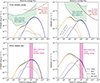 |
Fig. A.1. Predicted muon neutrino energy flux (left) and number flux (right) for the two UHE neutrino source candidates discussed in the main text. The emission of neutrinos above 1 PeV is led by interactions with broad line photons (orange) and above 10 PeV by interactions with the thermal photons from the dust torus (purple). The dashed gray curves show the neutrino emission expected without external photons (corresponding to a true BL Lac). In the upper panel, we show in green the 68% CL limits on the ten-year point-source flux from the direction of TXS 0506+056 under the assumption of a hard signal spectrum (Rodrigues et al. 2024b) and in red the latest IceCube ultra-high-energy flux limits (4π νFν/3, where νFν is the all-flavor diffuse flux in erg s−1sr−1cm−2, Abbasi et al. 2025). The pink band in the bottom panel is the energy range of the KM-230213A muon detected by KM3NeT (Aiello et al. 2025). |
A.1. High-energy neutrino events from blazar candidates
Here, we discuss briefly the model results in the context of the 170922A alert event detected by IceCube in 2017 from the direction of TXS 0506+056. After traveling an unknown distance in the ice, the detected muon deposited an energy of (23.7 ± 2.8) TeV in the detector. This value represents a lower bound on the energy of the muon produced by the signal neutrino. Assuming a power-law signal of E−2.13, the IceCube Collaboration (2018) derived a most likely true neutrino energy of 290 TeV. As recently shown by Kuhlmann & Capel (2025), however, this estimate is highly dependent on the assumed spectral shape of the neutrino signal. Generally, the neutrino spectrum predicted by leptohadronic scenarios tends to follow a hard power law. As we can easily see in the right panels of Fig. A.1, our predicted spectrum is flat (approximated by dN/dE ∼ Eγ with γ = 0) up to 100 TeV; then as interactions with BLR photons become viable it steepens to γ ≈ 1.2 between 1 and 100 PeV (γ ≈ 1.3 for PKS 0605-085), and cuts off exponentially above 100 PeV. Using the neutrino spectrum predicted by the single-zone model by Rodrigues et al. (2024b), with a maximum energy of 50 PeV, as a prior on the signal spectrum, Kuhlmann & Capel (2025) derive a most likely energy of about 30 PeV for the 2017 event. Although the precise value of this estimate depends on the specific spectrum predicted by the model, it is clear that in any UHE scenario, the 2017 neutrino has an energy in excess of 10 PeV. This implies that the muon was produced far from the detector and lost a large fraction of its energy in the ice before reaching the detector’s instrumented volume. This detection is thus only viable for blazars lying close to the experiment’s horizon, as is the case of TXS 0506+056. We leave a more detailed event-by-event analysis for future work.
For blazars lying considerably below the experiment’s horizon, detection of UHE neutrinos becomes challenging, requiring extremely high intrinsic fluxes due to the neutrinos’ efficient attenuation when crossing the Earth. Instead, as we showcase in Appendix B, considerably below its horizon the experiment is more likely to detect blazars emitting neutrinos in the PeV range, to which the Earth is less opaque.
Appendix B: Application to 3HSP J1528+2004, an IceCube candidate in the Northern Sky
Neutrinos in the UHE range suffer considerable attenuation when propagating through the Earth, and an experiment’s effective area is therefore considerably reduced for very up-going UHE neutrinos (Abbasi et al. 2023). An UHE blazar model therefore implies that viable candidates should lie relatively close to the experiment’s horizon, where the neutrinos will be near-horizontal and therefore Earth-skimming. For sources lying considerably below the experiment’s horizon, the reduced UHE effective area increases the neutrino signal flux required for detection.
In the main part of this paper, we apply the model to two candidate sources lying close to the horizon of their respective experiment. We now apply the model to an IceCube candidate blazar in the Northern Sky. Source 3HSP J1528+2004 is an HSP blazar lying at redshift 0.52 (Chang et al. 2019). The source has been identified as a masquerading BL Lac (Padovani et al. 2022) and is associated to a high-energy IceCube alert in the 9.5 year IceCube data (Abbasi et al. 2022b) together with 32 other candidate blazars identified by Giommi et al. (2020). With a declination of +20°, the neutrinos from this source are up-going in IceCube, which leads to considerable attenuation of the signal in the UHE range.
The best-fit result was obtained by fitting the extended jet model parameters to (multi-epoch) multiwavelength data, as done previously for the same source under a single-zone framework (Rodrigues et al. 2024b). As before, the green band in Fig. B.1 shows the 68% CL flux limits from the source’s direction (Rodrigues et al. 2024b). We can see that in this source’s case, the lower limit for the point-source signal strength shoots up above PeV. This follows from the fact that this source is well below IceCube’s horizon, thus requiring a high intrinsic neutrino flux in order to compensate for the strong attenuation suffered at UHEs. Unlike for the two UHE candidates discussed in the main text, here we explicitly reject any solution that undershoots the point source flux lower limits, in order to explicitly test whether the model can describe neutrino emission from a candidate lying below the experiment’s horizon. This requirement forces the optimization process to search a larger parameter space.
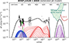 |
Fig. B.1. Extended jet model applied to IceCube candidate blazar 3HSP J1528+2004 (data taken from Rodrigues et al. 2024b, see references therein). The curves are color-coded as in Fig. 2. |
The predicted emission is shown in Fig. B.1; the best-fit jet profile is shown in the right panels of Fig. C.2. We can see that the predicted neutrino spectrum now peaks at only 3 PeV. This is the maximum energy for which a fit was found that respects the IceCube point-source limits. As detailed in Table 1 and Fig. C.2, this comes from a faster dissipation of the total magnetic field strength, B′∝r−1.17, compared to r−1.06 and r−1.04 for the two previous sources, which leads to a maximum proton energy at only the PeV level. The respective proton synchrotron emission peaks in the MeV range, which is currently unconstrained. The emission from hadronic cascades dominates the spectrum from soft X-rays up to 100 GeV (see the spectral decomposition plot in the bottom panel of Fig. C.1). Interestingly, synchrotron emission by the secondary pairs generated in hadronic cascades contributes significantly to the perceived peak of the optical-to-X-ray emission, which in this source lies at 1016.9 Hz. Emission from primary electrons peaks at only 1014 Hz, owing to our assumed weak energy dependence of the diffusion (Section 2.2). In this framework, the source is intrinsically an LSP/ISP, and the secondary contribution from hadronic cascades contributes to raising the total synchrotron peak frequency. More detailed modeling and time-domain correlation studies between the optical and X-ray emission are needed to eventually test this type of HSP model.
We conclude that the flexibility of the model in terms of the range of possible neutrino energies allows it to accommodate blazar candidates associated to highly up-going neutrinos by selecting jet properties that lead to a PeV-scale scenario rather than an UHE one. This highlights the fact that the extended jet model presented here is not intrinsically an UHE model; instead, UHE neutrinos emerge only within a subset of the jet parameter space.
With this flexibility, however, comes an inherent degeneracy in the space of viable model solutions. A promising approach to break this degeneracy would be applying the model to broad blazar samples within a unified physical framework, fitting it not only to the individual source data but also the collective emission from the population. Such a global framework, albeit challenging, may be key in providing models with the highly needed predictive power regarding the likelihood of each blazar as a viable neutrino candidate. The future joint operation of IceCube and the completed KM3NeT detector will also be invaluable in this context.
Appendix C: Further details on the extended jet model implementation
The jet is a continuous flow of particles, Poynting flux, and nonthermal radiation. We sample this flow at discrete locations along r, which is the distance to the supermassive black hole, and consider the jet to be symmetrical around this axis. At each location ri, we consider a spherical stationary zone and assume that a steady flow crosses that volume, which will lead to a steady-state radiative emission. We calculate this emission with the numerical approach summarized below, leading to a prediction for the steady-state nonthermal and neutrino emission at location ri. Finally, we sum the emitted fluxes over all the sampled locations, applying appropriate weights to ensure geometric and energetic consistency, leading to a global prediction for the continuous jet emission. This approach allows us to generalize the well-understood single-blob steady-state formalism (see e.g. Gao et al. 2019; Rodrigues et al. 2024a, 2018), to capture the extended nature of the jet. We now describe in greater detail each of these model components.
We simulate Ndec = 30 zones per decade in r, equally spaced in log(r). It is important to note that the jet parameters are given by continuous functions of r as detailed in Section 2.1; thus, the number of simulated zones does not impact the number of free parameters of the model, but only the computational cost of the simulation (each zone requires a few CPU-seconds). Through experimentation, we have determined that Ndec = 30 offers sufficient spatial resolution to accurately capture the system’s multiscale behavior. For lower values of Ndec, we would under-sample the jet emission, leading to an erroneous emission prediction. For higher values of Ndec, the result does not change, because we scale down the total photon and neutrino emission resulting from the sum of the individual simulations to account for their number and discrete nature, and to ensure energetic consistency. That down-scaling procedure is detailed at the end of this section.
For each location ri, we calculate the local magnetic field strength, turbulent magnetic field fraction, bulk Lorentz factor, and particle flux, which emerge from the assumed profile of the magnetic field dissipation, matter density profile, and energy conservation listed in Table 1. We then consider a stationary spherical zone with radius given by the jet cross-section radius at point ri, Rj[ri, Γj(ri)]. We make the approximation that the magnetic field and bulk plasma velocity are homogeneous across the volume of this spherical zone, justified by the fact that in general, Rj(r)≪r.
We calculate the particle interactions in each of the stationary zones using the open-source numerical code AM3 (Klinger et al. 2024), in an approach similar to previous single-zone steady-state models (see Rodrigues et al. 2024a,b, for recent implementations). The code numerically solves the time- and energy-dependent continuity equations describing a coupled system of photons, electrons, protons, as well as secondary species produced in electromagnetic and hadronic interactions, namely positrons, pions, and muons, as well as the neutrinos emitted through pion and muon decay. The general equation for particle species i has the form
![Mathematical equation: $$ \begin{aligned} \partial _{t^{\prime }}\, n_i(E^{\prime }, t^{\prime }) =&-\partial _{E^{\prime }} \left[\partial _{t^{\prime }}{E^{\prime }}(E^{\prime }, t^{\prime }) n_i(E^{\prime }, t^{\prime }) \right]\\&- \alpha (E^{\prime }, t^{\prime }) n_i(E^{\prime }, t^{\prime }) \,+\, Q_i^{\prime }(E^{\prime }, t^{\prime }), \nonumber \end{aligned} $$](/articles/aa/full_html/2026/02/aa56986-25/aa56986-25-eq41.gif) (C.1)
(C.1)
where ∂t′E′(E′,t′) represents continuous energy losses, such as through synchrotron emission, α(E′,t′) represents disappearance due to physical escape from the region and particle-annihilating interactions, such as photon-photon annihilation, and Qi′(E′,t′) represents the rate of particle injection. To emulate continuous acceleration of protons and electrons, we include constant injection terms Qe′(γ′e) and Qp′(γ′p) of the form dQ′e, p/dγe, p′∼γe, p′ − p, where γ′e, p = E′/(me, pc2). The spectrum falls to zero below γe, p′min and has an exponential cutoff above γe, p′max. The spectral index p is directly tested as a model parameter, considered constant along the jet and is the same for electrons and protons, since both are accelerated by the same leading mechanism. The four values of γe, p′min, max, on the other hand, are calculated self-consistently for each location ri based on the local values of the jet Lorentz factor, magnetic field, turbulence fraction, and so on (cf. Sect. 2.2). In turn, those local parameter values are calculated based on the overall evolution of the magnetic field strength, the environment particle density, and so on, as a continuous function of r, as controlled by the model parameters listed in Table 1 (cf. Sect. 2.2). Finally, the normalization of the proton and electron injection is given by  , where
  are given by Eqs. (8) and (9). It is worth highlighting that the proton and electron luminosities L′e, p(ri) are not parameterized, but arise from the combination of the local nonthermal particle fluxes Ṅe,p and the self-consistently estimated maximum energies γe, p′maxme, pc2.
Beside protons and electrons, the other explicit injection term is that for external photons, Qγext(Eγ). This accounts for the fact that the inner jet is exposed to photon fields from the BLR (including hydrogen and helium broad lines and a fraction of the thermal continuum from the accretion disk that gets isotropized in the BLR) and from thermal emission from the dusty torus. The local external photon density in the jet rest frame varies as a function of r, because (1) outside the BLR the local density of BLR photons decays quickly with r (and likewise for the dusty torus), and (2) the relative Doppler factor by which the photons are relativistically boosted into the jet frame depends on the local bulk Lorentz factor Γj(r) and the angle of incidence of the photons compared to the axis of jet motion. Thus, at a given location ri, we estimate the local density of BLR and dust photon fields in the jet rest frame, following the same treatment as in the single-zone model by (Rodrigues et al. 2024b). We assume a covering factor of 0.1 for the BLR and of 0.3 for the dusty torus. For TXS 0506+056 and 3HSP J1528+2004, we consider the best-fit value of the disk luminosity as listed in Rodrigues et al. (2024b), and scale the BLR and dusty torus radii as described in that work. The resulting photon density spectra in the jet frame are then interpolated into the simulation’s discrete photon energy array and included in the photon continuity equation in two ways: (1) an initial condition value dnγ/dE′γ(t′ = 0) = dnγext/dE′γ, and (2) a constant injection term Q′γ(Eγ′) = (c/R′j)(dnγext/dE′γ).
For neutral particles, such as photons, neutrons, and neutrinos, we include an energy-independent sink term representing speed-of-light escape: α = tesc′=R′j/c. For charged particles, we consider an energy-dependent escape term4α(E′) = tesc′(E′,δ), as described in Section 2.2, where δ is the exponent quantifying the energy dependence of the diffusion, and an adiabatic cooling term ∂tE′=E′c/(3R′j). Because in the radiative region the jet is narrowly focussed, adiabatic cooling is typically subdominant compared to other cooling processes.
Because we consider energy-dependent diffusion, only a fraction of the highest energy protons picked up by the jet locally, can efficiently propagate downstream. For electrons, downstream propagation in the inner jet is even more severely limited owing to the strong synchrotron losses. Thus, in this model, steady-state emission is typically dominated by the locally accelerated particles, and the contribution from particles diffusing downstream can therefore be neglected.
With the initial conditions, the injection terms, and the sink coefficients defined, we numerically solve the system in increments of Δt′ = 0.1Rj′/c, up to t′ = 3R′/c. At that stage, the radiation and particle densities provide a good approximation to the steady state, i.e., the asymptotic state when injection, escape, and radiative cooling balance out, yielding ∂t′ni → 0.
Once the steady-state photon and neutrino luminosity spectra emitted by each zone are obtained, a correction factor is applied to account for the discrete nature of the simulation, ensuring an accurate representation of the overall emission from the continuous jet.
The extended jet model is characterized by a constant total jet luminosity, r dLj/dr ≡ Lj, as shown in Fig. 2c. In considered setup, we simulate discrete, logarithmically spaced zones, and therefore sample the jet emission at a rate dN/dr = Ndec/[rln(10)]. We denote by Lsim the luminosity injected in each discrete simulation in the form of particles and magnetic field. The corresponding jet luminosity can be calculated as Lj ≡ rdL/dr = r(dN/dr)Lsim = [Ndec/ln(10)]Lsim. Thus, if we were to simply add the emission from each individual simulated zone, we would be overestimating the jet emission by a factor Ndec/ln(10). We therefore scale down the emitted steady-state photon and neutrino emission spectra νFν, as obtained from each discrete simulation, by a factor Lj/Lsim = ln(10)/Ndec ≈ 0.08(Ndec/30)−1. This ensures that the predicted emission is consistent with the assumed jet luminosity.
For the flare model applied to the 2017 flare of TXS 0506+056, as described in Section 3, we assume that additionally to the steady-state emission from the continuous flow, there is additional particle injection at an increased rate  , at a single location rflare. This emulates, for example, a simple scenario where a star crosses the jet perpendicularly to the direction of the flow, thus increasing temporarily the available number of particles. The parameters controlling the maximum energy and the time-dependent interactions of these particles are given by the same jet evolution equations applied to rflare, because the flare takes place in the same environment as the continuous emission. Thus, in this simple model, the flare introduces only two additional parameters compared to the steady-state emission: rflare and
  . The total emitted fluxes are then compared to the simultaneous multiwavelength data, thus constraining the two flare parameters.
Once we calculate the emission from each jet segment and scale down the flux as described above, we perform three additional operations. First, we apply relativistic boosting to estimate the photon and neutrino flux in the observer’s frame: (EdN/dE)obs = δD3 (dL′/dE′)/(4πDL2), where δD(r) = [Γj(r)(1 − β(r)cos θobs)]−1 is the Doppler factor of each zone and DL is the luminosity distance. For simplicity, we assume the same observation angle θobs along the jet, as listed in Table 1. Secondly, we scale the energy of the observed photons and neutrinos from each zone: Eobs = δDE′/(1 + z). Thirdly, we calculate the attenuation undergone by the emitted γ-rays during propagation due to interactions with the extragalactic background light (EBL). We use the energy-dependent flux attenuation prescription provided in the gammapy software (Donath et al. 2023), assuming the EBL specturm by Dominguez et al. (2011).
We neglect the electromagnetic emission emitted during propagation due to inverse Compton scattering on the EBL, which may lead to an additional cascade contribution. The respective flux depends on the strength of the intergalactic magnetic field (IGMF), the source’s redshift, and the extent of the time window, as quantified recently by Crnogorčević et al. (2025). At the same time, we can see from Fig. C.1 that in the case of TXS 0506+056 and PKS 0605-085, the unattenuated photon flux integrated above 100 GeV is lower than the integrated flux between 1 keV and 100 GeV. Thus, the observed flux should be dominated by the source emission (including the in-source cascades shown as dotted curves), while the EBL cascades should be sub-dominant, even if the electrons are not efficiently deflected by the IGMF. In the case of source 3HSP J1528+2004 (bottom panel of Fig. C.1), the unattenuated flux above 100 GeV is comparable to that below, so an additional contribution from EBL cascades may be an important factor to consider in future studies.
We evaluate the goodness of fit of each result by estimating a reduced chi-squared value between the logarithm of the observed and predicted fluxes. We first bin the multiwavelength data into logarithmic frequency bins of width Δ(log10ν) = 0.4. In each bin i, we estimate the weighted average of the observed flux, ⟨log10νFν, i⟩, and the total uncertainty on the flux σlog, i by accounting for the total variability inside the bin, as well as the individual uncertainties on each data point (cf. Rodrigues et al. 2024b, where the same method is described in greater detail). This treatment helps exclude the intrinsic source variability inside each given frequency band from the chi-squared calculation. However, where we fit steady-state emission, the data in each wavelength do not necessarily represent all possible states of the source. This introduces an additional variability that is not removed from the chi-squared calculation by this binning process.
After binning the data, we calculate the reduced chi-squared in logarithmic space:
![Mathematical equation: $$ \begin{aligned} \chi ^2_r\,=\, \frac{1}{N_\mathrm{bins} -N_\mathrm{pars,11} }\sum _i\frac{[\langle \log _{10}\nu F_{\nu ,i}\rangle -\log _{10}\nu \mathcal{F} _{\nu ,i}]^2}{\sigma ^2_{\log ,i}}, \end{aligned} $$](/articles/aa/full_html/2026/02/aa56986-25/aa56986-25-eq46.gif) (C.2)
(C.2)
where Npars = 11 is the number of free model parameters and log10νℱν, i is the logarithmic photon energy flux predicted by the model, interpolated on the central frequency of the i-th data bin. The resulting values of χr2 are listed in Table 1.
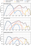 |
Fig. C.1. Predicted multiwavelength spectra from TXS 0506+056 (upper plot: see Fig. 2), PKS 0605-085 (middle: see Fig. 3), and 3HSP J1528+2004 (lower panel: see Fig. B.1). All photon fluxes are given in the observer’s frame, as in the main text, but here the effect of EBL attenuation is not included. The fluxes are divided into the different processes where they originate, according to the legend above. |
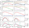 |
Fig. C.2. Parameter evolution of the extended jet model fit to sources PKS 0605-085 and 3HSP J1528+2004. The predicted spectra are shown in Figs. 3 and B.1, respectively. The same evolution plots are shown for TXS 0506+056 in Fig. 3c-g. |
In Fig. C.1, we show the calculated multiwavelength fluxes from the three sources included in this study. We separate the photon fluxes by the nonthermal process where they originate. We can see that in all three sources, proton synchrotron is significant. In the two sources that have proven viable UHE neutrino candidates (TXS 0506+056 and PKS 0605-085), proton synchrotron peaks above 100 MeV and extends up to the GeV range. The collective emission from hadronic cascades contributes a significant flux from X-rays up to 10 TeV. Attenuation on the EBL during propagation then leads to a cut-off of the observed spectrum at ∼100 GeV, as plotted in the other figures throughout this manuscript.
In all three fits, the inverse Compton emission by primary electrons is relatively inefficient. This feature is due to the low density of the radiation fields in the jet, particularly at the parsec scale. However, since the high-frequency emission is dominated by protons in all cases, the model is effectively insensitive to the electron inverse-Compton component. This feature therefore does not provide a meaningful constraint on the model and cannot be robustly predicted.
All Tables
All Figures
|
Fig. 1. Two scenarios of diffusion and acceleration. Upper panel: Diffusive shock acceleration with a diffusion coefficient D′E ∼ E′ − 1. Lower panel: Stochastic acceleration with D′E ∼ E′0.3. The timescales are given for the wide range of parameters η, B′, and R′j expected at distances 1017 cm ≲ r ≲ pc, as detailed in the main text. Black crosses show the maximum energy of electrons and protons predicted by the respective scenario. Green bands show the allowed range of E′e and E′p necessary to describe the multimessenger data. |
| In the text | |
|
Fig. 2. Extended jet model applied to the IceCube candidate blazar TXS 0506+056, fitted to the average multiwavelength emission (panel a, data taken from Rodrigues et al. 2024b, see references therein) and during the 2017 flaring event (panel b, data in magenta taken from IceCube Collaboration 2018; Keivani et al. 2018). The top panels show the best-fit spectra. The color curves show the photon emission by primary electrons (blue), photon emission by protons (red), and muon neutrino emission (purple) from the successive zones along the jet. The dashed curves in panel b show the emission from the flare zone. The black curves show the total emission. The green band shows the 68% CL limits on the neutrino point source flux from the source (Rodrigues et al. 2024b), and the dark red curve the UHE sensitivity of IceCube-Gen2 (Aartsen et al. 2021). The pink curve shows the BLR and accretion disk continuum emission, and the bright green curve the host galaxy contribution (see Rodrigues et al. 2024b). In panels c–g, we show the evolution along the extended jet of the jet energetics (c), dynamics (d), particle profile (e) and emission (f, g). |
| In the text | |
|
Fig. 3. Extended jet model applied to KM3NeT candidate blazar PKS 0605-085. Data adopted from Rodrigues et al. (2024a, see references therein). The curves are color coded as in Fig. 2. The magenta band shows the muon energy of the event KM-230213. |
| In the text | |
|
Fig. A.1. Predicted muon neutrino energy flux (left) and number flux (right) for the two UHE neutrino source candidates discussed in the main text. The emission of neutrinos above 1 PeV is led by interactions with broad line photons (orange) and above 10 PeV by interactions with the thermal photons from the dust torus (purple). The dashed gray curves show the neutrino emission expected without external photons (corresponding to a true BL Lac). In the upper panel, we show in green the 68% CL limits on the ten-year point-source flux from the direction of TXS 0506+056 under the assumption of a hard signal spectrum (Rodrigues et al. 2024b) and in red the latest IceCube ultra-high-energy flux limits (4π νFν/3, where νFν is the all-flavor diffuse flux in erg s−1sr−1cm−2, Abbasi et al. 2025). The pink band in the bottom panel is the energy range of the KM-230213A muon detected by KM3NeT (Aiello et al. 2025). |
| In the text | |
|
Fig. B.1. Extended jet model applied to IceCube candidate blazar 3HSP J1528+2004 (data taken from Rodrigues et al. 2024b, see references therein). The curves are color-coded as in Fig. 2. |
| In the text | |
|
Fig. C.1. Predicted multiwavelength spectra from TXS 0506+056 (upper plot: see Fig. 2), PKS 0605-085 (middle: see Fig. 3), and 3HSP J1528+2004 (lower panel: see Fig. B.1). All photon fluxes are given in the observer’s frame, as in the main text, but here the effect of EBL attenuation is not included. The fluxes are divided into the different processes where they originate, according to the legend above. |
| In the text | |
|
Fig. C.2. Parameter evolution of the extended jet model fit to sources PKS 0605-085 and 3HSP J1528+2004. The predicted spectra are shown in Figs. 3 and B.1, respectively. The same evolution plots are shown for TXS 0506+056 in Fig. 3c-g. |
| In the text | |
Current usage metrics show cumulative count of Article Views (full-text article views including HTML views, PDF and ePub downloads, according to the available data) and Abstracts Views on Vision4Press platform.
Data correspond to usage on the plateform after 2015. The current usage metrics is available 48-96 hours after online publication and is updated daily on week days.
Initial download of the metrics may take a while.