| Issue |
A&A
Volume 706, February 2026
|
|
|---|---|---|
| Article Number | A302 | |
| Number of page(s) | 11 | |
| Section | Extragalactic astronomy | |
| DOI | https://doi.org/10.1051/0004-6361/202557017 | |
| Published online | 18 February 2026 | |
JWST-discovered AGN: Evidence of heavy obscuration in the type 2 sample from the first stacked X-ray detection
1
INAF – Osservatorio di Astrofisica e Scienza dello Spazio di Bologna (OAS) Via Gobetti 93/3 I-40129 Bologna, Italy
2
Dipartimento di Fisica e Astronomia (DIFA), Università di Bologna Via Gobetti 93/2 I-40129 Bologna, Italy
3
Department of Physics and Astronomy, Clemson University, Kinard Lab of Physics Clemson SC 29634, USA
4
Kavli Institute for Cosmology, University of Cambridge Madingley Road Cambridge CB3 OHA, UK
5
Cavendish Laboratory – Astrophysics Group, University of Cambridge 19 JJ Thomson Avenue Cambridge CB3 OHE, UK
6
Department of Physics and Astronomy, University College London Gower Street London WC1E 6BT, UK
7
Max-Planck-Institut für extraterrestrische Physik (MPE) Gießenbachstraße 1 85748 Garching, Germany
8
Dipartimento di Fisica e Astronomia, Università di Firenze Via G. Sansone 1 I-50019 Sesto Fiorentino Firenze, Italy
9
INAF – Osservatorio Astrofisico di Arcetri Largo Enrico Fermi 5 I-50125 Firenze, Italy
★ Corresponding author: This email address is being protected from spambots. You need JavaScript enabled to view it.
Received:
28
August
2025
Accepted:
21
December
2025
Abstract
One of the most puzzling properties of the high-redshift active galactic nucleus (AGN) population recently discovered by JWST, including both broad-line and narrow-line sources, is their X-ray weakness. With very few exceptions, and regardless of the optical classification, they are undetected at the limits of the deepest Chandra fields, even when stacking signals from tens of sources in standard observed-frame energy intervals (soft, hard, and full bands). It has been proposed that their elusive nature in the X-ray band is due to heavy absorption by dust-free gas or an intrinsic weakness, possibly due to high super-Eddington accretion. For this work we performed X-ray stacking in three customized rest-frame energy ranges (1–4, 4–7.25, and 10–30 keV) of a sample of 50 type 1 and 38 type 2 AGN identified by James Webb Space Telescope (JWST) in the Chandra Deep Field South (CDFS) and Chandra Deep Field North (CDFN) fields. For the type 2 subsample, we achieve a total exposure of about 210 Ms, and report a significant detection (∼3σ) in the hardest band (10–30 keV rest frame), along with relatively tight upper limits in the rest-frame softer energy bands. The most straightforward interpretation is in terms of heavy obscuration due to gas column densities well within the Compton-thick regime (> 2 × 1024 cm−2) with a large covering factor, approaching 4π. The same procedure applied to the type 1 subsample returns no evidence of a significant signal in about 140 Ms stacked data in any of the adopted bands. The bolometric correction kbol to the absorption corrected 2–10 keV X-ray luminosity of type 2 AGN is consistent with the average value obtained for X-ray selected type 2 objects in the literature. The lower limit on kbol for the type 1 sample is significantly higher and inconsistent with that of type 2 objects. Absorption in the Compton-thick regime or extreme X-ray weakness, would bring the current lower limits closer to the observed values for type 1 X-ray selected AGN. A brief comparison with the current observations and the implications for the evolution of AGN are discussed.
Key words: galaxies: active / galaxies: high-redshift / quasars: general / quasars: supermassive black holes
© The Authors 2026
 Open Access article, published by EDP Sciences, under the terms of the Creative Commons Attribution License (https://creativecommons.org/licenses/by/4.0), which permits unrestricted use, distribution, and reproduction in any medium, provided the original work is properly cited.
This article is published in open access under the Subscribe to Open model. This email address is being protected from spambots. You need JavaScript enabled to view it. to support open access publication.
1. Introduction
Several surveys with the James Webb Space Telescope (JWST) have discovered a population of high-redshift (z ∼ 4 − 10) active galactic nuclei (AGN) with bolometric luminosities significantly lower (< 1045 erg s−1) than previously observed in bright quasars dominating the AGN population at high redshift. Most of them have been identified via the detection of relatively broad emission lines with Hα widths on the order of 2000 km s−1, and are thus classified as type 1 AGN (e.g., Maiolino et al. 2024b, Juodžbalis et al. 2025, hereafter J25). Their black hole mass estimates range from 106 to 108 M⊙ (e.g., Maiolino et al. 2024a; Kocevski et al. 2023). They tend to be over-massive compared to the stellar masses of their host galaxies, and with respect to the local relation, suggesting a vigorous growth phase at early times (although this interpretation is still debated; see Ananna et al. 2024). About 10 − 30% of them (Hainline et al. 2025) are dubbed little red dots owing to their point-like appearance and red near-infrared colors; in addition to broad permitted lines, they are characterized by a V-shaped continuum, with a relatively blue UV slope (e.g., Kocevski et al. 2025). Additionally, a growing number of narrow-line type 2 AGN are identified using several diagnostic diagrams for the emission line, some specifically developed for the classification of the emission lines at high redshift (Scholtz et al. 2025; Mazzolari et al. 2025; Calabrò et al. 2023). The space densities of these newly JWST-discovered AGN at z ∼ 4 − 6 are about one to two orders of magnitude higher than the extrapolation of the quasars luminosity function and of the X-ray selected AGN luminosity function (e.g., Harikane et al. 2023; Matthee et al. 2024; Greene et al. 2024; Maiolino et al. 2024a; Juodžbalis et al. 2025) suggesting that JWST is tracing the emergence of a new population that is much larger than the most optimistic (Giallongo et al. 2015) estimates from the X-ray-selected AGN. Given that known X-ray-emitting AGN account for some 80 − 90% of the X-ray background (e.g., Moretti et al. 2003; Cappelluti et al. 2017), it is not surprising that this new population is X-ray silent. Although many examples of X-ray weak quasars were reported in the literature (Risaliti et al. 2001) well in advance the JWST surveys, the JWST population is much larger. Even more intriguing, this new population remains undetected even with stacking techniques performed in deep X-ray observations such as those in the Chandra Deep Fields (Yue et al. 2024, Mazzolari et al. 2024, Maiolino et al. 2025, hereafter, M25).
Two broad classes of models were proposed to explain the X-ray weakness. The first is super-critical accretion resulting in an extremely soft X-ray spectrum (e.g., Pacucci & Narayan 2024; Madau & Haardt 2024; Madau 2025; Maiolino et al. 2025) and significant absorption at high inclinations due to self-shadowing. The second class is heavy obscuration with a high covering factor and column densities exceeding 1024 cm−2 by dust free–poor gas to account for the presence of broad lines and UV emission (e.g., M25, Ji et al. 2025, Juodžbalis et al. 2024).
In the first case, the steep X-ray emission explains the lack of detection in the observed standard (0.5 − 2 and 2 − 7 keV) bands corresponding, approximately, to 4–40 keV rest frame. The heavy absorption hypothesis implies that the X-ray flux is dimmed by obscuration, especially in the soft band. For optical depths on the order of τ ≫ 1 and large covering factors, the signal in the hard X-ray band may also be strongly suppressed.
In order to understand which physical mechanism is more likely to explain the observed properties, we carried out a Chandra stacking analysis at the positions of the sources in our sample in several energy intervals, tuned to detect characteristic features of heavy absorption, such as a very hard X-ray spectrum emerging at > 8 keV, enhanced emission around the iron line complex at ∼6 − 7 keV and–or the presence of a strong soft excess below about 1 keV. A detection in the stacked signal in the softest energy channels would be suggestive of a steep spectrum, possibly related to supercritical accretion, while a signal at the hardest energies would favor the heavy obscuration interpretation. In principle, it is possible to constrain the average column densities, owing to the strong dependence of the X-ray flux upon the optical depth for Compton scattering. The present work takes a step further with respect to previous analyses based on the search for a stacked signal in deep Chandra fields as we explicitly stack emission from all sources in the samples in the same rest-frame bands, and fully exploit the stacked X-ray SED shapes to estimate the absorption levels.
The paper is organized as follows. In Section 2 the sample selection is presented. In Section 3 we describe the procedure adopted to analyze (stack) the X-ray data. In Section 4 we present our results. In Section 5 we discuss the implications of our results in light of the current models of the X-ray and multiband properties of JWST AGN and draw our conclusions. Errors and upper limits are reported at the 68% confidence level, while the upper limits in Figure 5 are given at the 90% confidence. We adopt a flat cosmology with H0 = 67.7 km s−1 and Ωm = 0.307 (Planck Collaboration XIII 2016).
2. The JWST sample of AGN
Our parent sample is composed of AGN identified by JWST in the footprints of the GOODS-N and GOODS-S fields, the deepest Chandra fields, with a total exposure of about 2 and 7 million seconds, respectively. The choice is dictated by the need for deep X-ray exposures to obtain meaningful limits on the AGN X-ray emission. The optical classification as type 1 and type 2 AGN is mainly from the JWST Advanced Deep Extragalactic Survey (JADES; Eisenstein et al. 2025, D’Eugenio et al. 2025).
The type 1 AGN were identified based on the broad component in the Hα and Hβ emission with a full width at half maximum (FWHM) > 1000 km s−1 (Matthee et al. 2024), without a corresponding kinematical component in the [OIII] λλ5007,4960, hence ruling out an outflow origin. In total, this work yields a clean selection of 35 type 1 AGN in the GOODS-S and GOODS-N fields. We also considered the type 1 objects from the First Reionization Epoch Spectroscopically Complete Observations (FRESCO) survey (Oesch et al. 2023), the two little red dots at z > 7 in Xiao et al. (2025), and the broad Hα emitters in the JADES, FRESCO, and Complete NIRCam Grism Redshift Survey (CONGRESS) surveys selected by Zhang et al. (2025). The type 1 objects are published in J25 and also in M25. We refer to the discovery papers for further details on the selection and classification.
The type 2 AGN were selected from Scholtz et al. (2025), which is a pilot study to select type 2 AGN in the JADES survey. As such, it was only employed on the first two tiers of JADES observations, at that point only observed in GOODS-S. The emission line diagnostics used in the pilot study were the Baldwin et al. (1981) and Veilleux & Osterbrock (1987) diagrams, with selection criteria modified for high-z by Scholtz et al. (2025) to account for low-metallicity star formation, the HeII λ4686 diagrams (Shirazi & Brinchmann 2012), UV emission line diagnostics (Hirschmann et al. 2019), and the presence of high-ionization lines such as [NeIV] λ2424 and [NeV] λ3420. In total, this study selected 41 unique type 2 AGN in the regions of the GOODS-South field from a total of 209 galaxies covering the redshift range 2–9.5. The full selection of type 2 AGN from the JADES survey that will cover the GOODS-N field will be presented in Scholtz et al. (in preparation). The list of sources is reported in the Appendix in Tables A.1 (type 1) and A.2 (type 2). We only used the robust AGN candidate in the Chandra Deep Field South CDFS from J25 and removed the tentative candidates from our sample.
The sources’ X-ray emission is discussed in M25 and J25. A few sources were detected in the X-ray band and excluded from our sample. Two broad-line AGN (GN 721 and XID_4031) are relatively faint in the X-rays (kbol, X > 100, where kbol, X = Lbol/L2 − 10 keV), but with a hard X-ray spectrum consistent with Compton-thick obscuration (Gilli et al. 2014; Circosta et al. 2019). The absorption-corrected bolometric correction derived from Compton-thick obscuration is consistent with the observed distribution of standard type 1 AGN. Two additional broad-line AGN (GS_49729 and GS_209777) were detected with an unobscured X-ray spectrum (Γ ∼ 1.7) and average bolometric correction kbol, X ∼ 15, hence also consistent with standard type 1 AGN. One type 2 object (GS_21150) was X-ray detected, but with an insufficient number of photon counts to estimate the spectral shape. In the following, we consider the 38 type 2 and 50 type 1 AGN that are not individually detected, and that do not produce a significant stacked signal in the standard observed-frame soft (0.5–2 keV) and hard (2–7 keV) Chandra bands (M25).
The relevant data for the two samples are reported in Appendix A, and in Tables A.1 and A.2. The redshift distributions for the two samples are reported in the two panels of Figure 1. As a consequence of the JADES parent sample’s selection criteria, most sources are at z > 2, extending up to z ∼ 9. The median redshifts are z ∼ 4.2 for type 2 and z ∼ 5 for type 1.
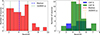 |
Fig. 1. Left: Redshift distribution for the type 2 AGN analyzed in this work, all from CDF-S. The median of the distribution is reported, as well as the 16th and 84th percentiles, as labeled. Right: Redshift distribution for the type 2 AGN analyzed in this work, from the CDF-S (blue) and CDF-N (green). The median of the distribution is reported, as well as the 16th and 84th percentiles, as labeled. |
For type 2 AGN, the bolometric luminosity is inferred from the extinction-corrected [O III]5007 line, adopting the scaling relation given in S25, and is reported in Table A.2 and Figure 6 (left). As can be seen in the figure, the bolometric luminosities span more than three orders of magnitude in the range log .
.
For type 1 AGN, the bolometric luminosity is inferred from the Hα luminosity, adopting the scaling relation provided by Stern & Laor (2012), and is reported in Table A.1. The bolometric luminosities of type 1 cover about three orders of magnitude, in a significantly higher Lbol interval with respect to type 2 AGN  . Figure 6 (right) only shows the type 1 AGN from M25, for which we have a direct estimate of the kbol, X.
The 38 type 2 AGN from S25 all lie in the CDFS, within 3.3 arcmin from the field center. Thus, we took advantage of the sharpest Chandra psf (90% encircled counts fraction always within 2.5 arcsec radius). The type 1 AGN in the Chandra Deep Field North (CDFN, 36 sources) lie in the central region of the field, within 3–4 arcmin of the aimpoint of the majority of the pointings, thus contributing to the total 2Ms exposure. Half of the type 1 AGN in the CDFS (7 sources) lie in the central 3 arcmin region of the field, while the other half are selected from different JWST pointings and are located between 4 and 7 arcmin (90% encircled counts fraction goes from 3 to 6 arcsec radius).
3. Data reduction and stacking procedure
To increase the sensitivity of the X-ray stacking analysis, we performed a stack in three adaptively chosen bands to test the hypothesis of heavy obscuration in the average spectrum of the sources in the sample.
The X-ray data in the Chandra deep fields were reduced and extensively analyzed by many authors. For the present paper, we rely on the data products (e.g., stacked event files, exposure maps, source catalogs) made available by the Penn State Chandra team2. We refer to Luo et al. (2017) and Xue et al. (2016) for all the details of the Chandra data analysis.
In order to obtain a robust estimate of the background, the detected sources from the Luo et al. (2017) catalog were removed from the event files, assuming circular regions whose radius is a function of the source intensity: from 4 pixels (2″) for < 30 full band counts to 6 pixels (3″) for bright > 100 counts sources. The adopted radii exclude 95 − 98% of the counts of the detected sources. This ensures < 1 count per source on average, leaking outside the excluded region. The local background was estimated in a box of 20 pixels on each side around the excluded regions. The masked pixels were then assigned random discrete values extracted from a Poisson distribution with the expectation value set to the median background counts per pixel, thus reproducing the same background levels. For each source to be stacked, square cutouts of 50 pixels were created around the input position.
The novelty of our approach with respect to previous works that stacked Chandra images at the position of known JWST sources lies in the careful selection of the energy bands where the stacking is performed. Specifically, we selected three rest-frame bands (1–4, 4–7.25, and 10–30 keV), corresponding to different observed bands depending on the redshift of each source included in the stacking. In the rest of the paper we refer to these bands as the soft band (SB, 1–4 keV), medium band (MB, 4–7.5 keV), and ultra-hard band (UHB, 10–30 keV). The 1–4 keV band was chosen to include the softest photons detectable by Chandra in the observed energy range, while we chose the 10–30 keV band as our hardest band after performing multiple tests3 that allowed us to determine that such an energy range is the best trade-off between the band width, to maximize the total counts, and the high-energy boundary, to minimize the background counts. We limited the MB to 7.25 keV, a trade-off between the band width and the expected spectral shape, which drops quickly, especially for obscured sources, above the iron K-edge.
The total stacked counts (Table 1) are extracted from a circular region centered at the optical JWST position with R = 2″, whereas the background counts are measured from an annular region with inner radius of 5″ and outer radius of 10″ and then rescaled for the background-to-source area ratio. The net source counts are then computed by subtracting the rescaled background counts from the total counts. The errors are propagated accordingly.
Stacking results for the type 1 and type 2 samples.
4. Results
The thumbnails associated with the rest-frame stack in the SB, MB, and UHB bands are shown in Figure 2 and Figure 3 for the type 2 and type 1 AGN, respectively. The background and source counts for both samples are reported in Table 1.
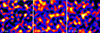 |
Fig. 2. Left: Type 2 stacked image 1–4 keV rest frame. Center: Type 2 stacked image 4–7.25 keV rest frame. Right: Type 2 stacked image 10–30 keV rest frame. |
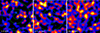 |
Fig. 3. Total (CDFS + CDFN) stacked images for the type 1 sample. Left: 1–4 keV SB. Center: 4–7.25 keV MB. Right: 10–30 keV UHB. |
The AGN in the type 1 sample were not detected in any rest-frame bands. The sources in the type 2 AGN sample were not detected in the SB and MB (as defined above), while they were detected in the UHB, with significance (1 − PB) = 0.9996 using Poisson statistics (0.9993 with Gaussian statistics). We also considered the possibility that the UHB signal is due to a specific subset of sources. Several tests were performed by dividing the type 2 sample according to their redshift, bolometric luminosity, and expected X-ray flux, for a given bolometric luminosity and redshift, assuming the standard X-ray bolometric correction from Duras et al. (2020). The tests were performed using only two bins due to the low number of candidates. There is no evidence for a signal in any of the adopted bins, suggesting the lack of a trend with either redshift or luminosity.
The significance of the detection in the UHB was also tested via simulations. We generated 1000 realizations of the type 2 sample by randomizing the position of each source, in a region within one arcmin of the original position (to ensure exposure and background levels comparable with the real sources), and repeated the stack exercise. None of the realizations returns a number of counts higher than observed. The resulting detection significance is therefore > 0.999, that is, ≳3σ (Figure 4).
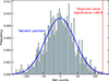 |
Fig. 4. Distribution of stacked net-counts in the UHB for 1000 realizations of random positions (cyan histogram). The number of stacked net counts obtained for the type 2 AGN sample is marked with the dashed red line. All of the random realizations return a lower number of net counts, implying a significance of > 0.999 of the stacked emission from the type 2 AGN sample. |
To convert stacked source counts into fluxes and then luminosities, we proceed as follows. First, we assume three different spectral models for the intrinsic emission, either a power law with Γ = 2 or a Compton-thick obscured model using the uxclumpy code (Buchner et al. 2019) with either NH = 2 × 1024 or NH = 1025 cm−2 (see below for details on the model parameters). Then we use an average instrumental effective area obtained from a position in the same region as the stacked sources, both for CDFS and CDFN. The response files account for the variation of Chandra response over time since it is computed as an average of the 102 pointings in the CDFS and the 20 pointings in the CDFN collected over time in the two fields. For each stacked object, we use its redshift to shift the intrinsic spectrum and convolve it with the effective area. This procedure allows us to obtain the expected distribution of detected photons in a given observed band corresponding to the SB, MB, and UHB rest-frame bands. We considered 1000 logarithmically spaced bins in the observed energy range 0.3–10 keV. The average expected photon energy is computed for each source and each band as ∑(Ei × Ni)/∑(Ni), and is translated into a corresponding average effective area for that source. The sample-averaged photon energy and effective area, weighted for the effective area contributions of each source (in terms of exposure times, the contributions are roughly the same for each source), are then estimated. For example, type 2 AGN in the UHB have average photon energies in the range 1.5 − 4.8 keV, and average effective areas in the range 210 − 400 cm2, and the sample averages are 3.3 keV and 268 cm2, respectively. The total exposure time is computed by stacking the values at the position of each source from the exposure maps of the two fields. The fluxes are then computed, at the average observed band, as F = (Counts × ⟨E⟩)/(Texp × ⟨Aeff⟩).
At the same time, the luminosities are estimated assuming the corresponding average redshift, without k-correction since the entire procedure is performed in the rest frame. Since exposures and effective areas are very different between CDFS and CDFN, the flux and luminosity limits in the CDFS and CDFN were computed separately.
The differences between fluxes and luminosities computed with an unabsorbed power-law spectrum and with a heavily absorbed one with NH = 2 × 1024 or NH = 1025 cm−2 are on the order of ∼20 − 30% in the SB and minimal in the MB and UHB, while they are negligible between the two Compton-thick cases; therefore, we report only the value for the NH = 2 × 1024 case in Table 2.
Flux and Luminosity limits.
We note that for the 1–4 keV band, a fraction of the rest-frame band moves below the Chandra low-energy limit of 0.3 keV for sources at z ≳ 2 (almost all our sources). When computing fluxes and luminosities, we must consider that only part of the intrinsic spectrum will be included in the observed band. We correct for this effect by computing the fraction of missing counts for each source for a given spectral shape. For example, if 70% of the intrinsic photons are expected to be missing below 0.3 keV, to recover the correct count rate the exposure time is decreased by 70%. This correction is larger for the unobscured power-law spectrum (a factor ∼2 on the final stacked flux and luminosity values) than for the Compton-thick obscuration case since the fraction of soft photons is much larger in the first case.
To estimate the spectral shape consistent with the stacking analysis results, we compared the detection in the UHB and the upper limits in the SB and MB with mock spectra for different obscuration values. The calculations used the physically motivated uxclumpy code (Buchner et al. 2019) in XSPEC. The model spectra cover a wide range of line-of-sight absorption column densities (log NH= 20–26 cm−2). Two components describe the geometry of the clumpy obscuring gas. A toroidal distribution of clouds with variable vertical extent and column density parameterized by its covering factor (model parameter TORsigma in the range 0–0.84), plus an additional Compton-thick reflector (log NH = 25.5 cm−2), which can be interpreted as part of the dust-free broad-line region, an inner rim, or a warped disk. The variable number of thick clouds parameterizes the covering factor of the ring (model parameter CTOR in the range 0–0.6). Given the very limited observational constraints, we fixed the slope of the primary continuum to Γ = 1.9, and the high-energy cutoff at Ecut = 200 keV. We also assume a line-of-sight inclination of 60 degrees, consistent with the type 2 classification of the sample.
Model spectra were computed for a range of column densities in the high absorption regime (log  ), and for a range of the TORsigma and CTOR parameters. In Figure 5, we report three model spectra representative of the various possible combinations of the parameters.
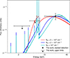 |
Fig. 5. Spectral models computed with the uxclumpy code described in (Buchner et al. 2019) rescaled to the observed 10–30 keV flux from the stacking analysis. We refer to the text for details on the model assumptions and geometry. The column density increases from 5 × 1023 cm−2 (red curve) to 2 × 1024 cm−2 (blue curve) and 1025 cm−2 (cyan curve). The UHB detection and the upper limits in the SB and MB are also reported. |
The red curve refers to a spectrum transmitted through a Compton-thin (NH = 5 × 1023 cm−2) gas with high covering factor (0.84) and without an inner ring. The blue curve is for a Compton-thick absorber (NH = 2 × 1024 cm−2) with the same assumptions for the covering factor and the inner ring. The green curve includes the inner Compton-thick ring (CTOR = 0.6) and is for a heavily obscured, NH = 1025 cm−2, clumpy torus with high covering factor (0.84). For sources with such large line-of-sight column densities, changes in the covering factor of the clumpy clouds (i.e., in the TORsigma parameter) do not significantly affect the observed spectral shape in the energy range sampled in this work.
The spectra are rescaled to the observed stacked flux in the 10–30 keV band. The upper limit in the 1–4 keV band is relatively loose, while the limit in the 4–7.25 keV band suggests that the average spectrum should steeply decline below the peak at ∼20 keV. This behavior favors Compton-thick absorption, almost independently of the details on the geometry of the clumpy absorber. Strong iron lines, with equivalent widths (EQWs) on the order of 1–2 keV, are a distinctive feature of Compton-thick absorption and are expected to contribute to the MB counts. In order to quantify their possible impact, we also tested the staking procedure in narrower bands centered at 6.4 keV, namely 5.8–7.2 and 6.0–6.8 keV. There is no evidence for a signal with upper limits of about 20 and 10 counts, respectively. Given the Chandra energy resolution and the intrinsic weakness of our sources, narrower bands are severely photon starved. A putative iron K line with EQW of 2 keV at the median redshift (z ≈ 4) of our sample would contribute to ∼20% to the measured flux in the MB band. On the basis of the above-described test, we conclude that a strong iron line is fully consistent with our upper limits.
5. Discussion and conclusions
The relatively tight upper limit in the MB coupled with the UHB detection indicates the obscured nature of JWST-selected type 2 AGN. The most straightforward interpretation is that they belong to the obscured population responsible for the X-ray background spectrum (Gilli et al. 2007). In this respect, their nature is not exotic or elusive; they represent the low-luminosity tail of the AGN population, which has already been observed and characterized at lower redshifts and higher luminosities. The bolometric to X-ray luminosity ratio is shown in the left panel of Figure 6 for the type 2 sample. The magenta star corresponds to the ratio computed assuming the observed 2–10 keV luminosity for Compton-thick (NH = 2 × 1024 cm−2) obscuration. This model is consistent with the upper limits in the SB and MB (blue curve in Figure 5). The bolometric correction corresponding to absorption-corrected luminosities for three different values of intervening absorption is also shown with thick black marks.
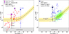 |
Fig. 6. Left: Ratio of the AGN bolometric luminosity and the X-ray luminosity as a function of the bolometric luminosity for type 2 AGN. The small brown points represent X-ray-selected type 2 AGN in COSMOS (Lusso et al. 2012). The red points are the lower limits obtained for each JWST type 2 source in M25. The magenta star shows the kbol obtained from the observed 2–10 keV luminosity derived from the 10–30 keV stacked detection assuming a Compton-thick spectrum with NH = 2 × 1024 cm−2 (blue curve in Figure 5), at the median Lbol of the sample. The horizontal error bar corresponds to the 16th and 84th percentiles of the observed distribution of bolometric luminosities in the stacked sample. The kbol corresponding to absorption-corrected intrinsic luminosities derived for NH of 5 × 10²³, 2 × 1024, and 1025 cm−2 is shown with the black error bars. The violet data point is equivalent to the magenta one, but Lbol is derived from [O III] using the Netzer (2019) bolometric correction. The X-ray-detected heavily obscured source XID 403 is shown with a blue diamond. The kbol, X from the de-absorbed luminosity is shown with the empty symbol. Right: Same as the left panel, but for type 1 AGN. The green and cyan small points represent X-ray-selected type 1 AGN in COSMOS from Lusso et al. (2012) and QSOs from Lusso et al. (2020). The blue points are lower limits and detections for type 1 sources in M25. The dark blue star indicates the kbol limit for the stacked type 1 sources in the CDFN obtained from the observed upper limits assuming a spectrum with Γ = 1.7. The black error bars were computed using the same assumptions as for the type 2 sample in the left panel. The horizontal error bar corresponds to the 16th and 84th percentiles of the observed distribution of bolometric luminosities in the stacked sample (see text for a more detailed description). In both panels, the black continuous line shows the kbol, X − Lbol relation from (Duras et al. 2020) while the gold area shows the scatter. The region below kbol = 1 is marked as unphysical as it would imply that L2 − 10 keV > Lbol. |
The points are plotted at the median bolometric luminosity of the sample. Extreme values (NH ≳ 1025 cm−2) of absorption are ruled out as they would be inconsistent with the definition of the bolometric correction. Combined with the limits obtained by the X-ray stacking, the most probable average value for the absorption is on the order of log NH ∼ 24.2 ± 0.3 cm−2. This constraint is mitigated if a different recipe for calculating the bolometric correction (Netzer 2019) is adopted, as indicated by the violet star and the corresponding error bar.
We conclude that the average bolometric correction of the type 2 AGN is consistent with the values already observed in the literature, reinforcing the hypothesis that the JWST-selected type 2 AGN do not significantly differ from their lower redshift and–or higher luminosity counterparts.
For comparison, we show the location of the two X-ray-detected and X-ray-obscured sources in the parent sample: the blue diamond is XID 403 (Gilli et al. 2014), where the kbol, X is estimated from the observed (filled) and absorption-corrected (empty) luminosities from Circosta et al. (2019). The green diamond is GN 721, detected at ∼5σ with a limited counting statistic in the CDFN (Maiolino et al. 2025). Its spectrum is flat (Γ ∼ 0.1), consistent with Compton-thick obscuration. However, due to the limited number of detected photon counts, a proper spectral analysis is not possible, and therefore the kbol, X from the de-absorbed luminosity cannot be derived. The two candidate Compton-thick broad-line AGN could represent the tip of the iceberg of a fainter and–or more obscured population.
A question arises from their abundance. If their space densities, at present ill-constrained, turn out to be much higher than those expected based on the extrapolation of the luminosity function at high redshift, then there might be tension with the observed intensity of the hard X-ray background. However, Comastri et al. (2015) showed that the current uncertainties on the level of the X-ray background around its peak at 20–30 keV are such that it is possible to accommodate a relatively large number of heavily obscured Compton-thick AGN with a spectrum similar to those reported in Figure 5. A more detailed investigation on the space density of type 2 AGN in various JWST surveys, including the effects of incompleteness, will be the subject of a future investigation.
The lack of detection in any band for type 1 confirms and extends previous claims about the puzzling nature of these objects. The upper limits in the rest-frame SB, MB, and UHB are larger than those for the type 2 sample due to the shorter total exposure (140 versus 209 Msec) and the fact that the majority of the type 1 sample is in the CDFN where the exposure is lower than in the CDF-S by a factor ∼3.5. The average bolometric correction for type 1 AGN in the CDFN is reported in the right panel of Figure 64. The observed upper limits allow for a relatively loose constraint on the average X-ray power-law slope (Γ ≤ 1.7 − 1.8). The blue star, plotted at the median bolometric luminosity of the sample, corresponds to the lower limit on the observed kbol assuming a spectrum with Γ = 1.7. The lower limits corresponding to absorption-corrected luminosities, for the same values of intervening absorption adopted for the type 2 sample, are also reported. The observed kbol lower limit for type 1 AGN is inconsistent with that measured for type 2 AGN. Heavy absorption, in the Compton-thick regime, would be needed to bring the lower limits within the region populated by the typical values of X-ray selected type 1 AGN. The X-ray weakness of type 1 AGN may be explained if these sources are accreting at rates exceeding the Eddington limit (Madau & Haardt 2024; Madau 2025). In these models, the X-ray luminosity is generated in the funnels of a geometrically thick accretion disk. The coronal plasma is cooled at lower temperatures than in standard thin disks. The emitted X-ray spectrum is extremely steep (Γ ≳ 3 − 4), making these sources undetectable, especially at high redshifts. We note that the Lbol range spanned by the individual data points from M25 and by our staked data points are different because the samples are different (we added new sources from J25; Zhang et al. 2025; Xiao et al. 2025, see Table A.1) and several Lbol values for the sources in common have been revised in J25.
A tighter constraint could be obtained by significantly increasing the sample size, especially in the CDFS. However, it should be noted that, at high redshift, the softest energies probed are on the order of a few kiloelectronvolts and thus the shape of the soft X-ray spectrum cannot be determined. As a consequence the hypothesis of an ultra-steep X-ray spectrum to explain the observed X-ray weakness (Madau & Haardt 2024) cannot be tested. Future deep and wide X-ray surveys, such as those planned by the AXIS mission concept (Reynolds et al. 2023), will probe the faint end of the luminosity function at high redshift (Marchesi et al. 2020) down to limiting fluxes one order of magnitude lower than Chandra deep surveys.
Acknowledgments
We thank the anonymous referee for their constructive report. This research was supported by the Munich Institute for Astro-, Particle and BioPhysics (MIAPbP), which is funded by the Deutsche Forschungsgemeinschaft (DFG, German Research Foundation) under Germany’s Excellence Strategy – EXC-2094 – 390783311. This research has made use of data obtained from the Chandra Data Archive, and software provided by the Chandra X-ray Center (CXC) in the application packages CIAO.
References
- Ananna, T. T., Bogdán, Á., Kovács, O. E., Natarajan, P., & Hickox, R. C. 2024, ApJ, 969, L18 [NASA ADS] [CrossRef] [Google Scholar]
- Baldwin, J. A., Phillips, M. M., & Terlevich, R. 1981, PASP, 93, 5 [Google Scholar]
- Buchner, J., Brightman, M., Nandra, K., Nikutta, R., & Bauer, F. E. 2019, A&A, 629, A16 [NASA ADS] [CrossRef] [EDP Sciences] [Google Scholar]
- Calabrò, A., Pentericci, L., Feltre, A., et al. 2023, A&A, 679, A80 [NASA ADS] [CrossRef] [EDP Sciences] [Google Scholar]
- Cappelluti, N., Li, Y., Ricarte, A., et al. 2017, ApJ, 837, 19 [NASA ADS] [CrossRef] [Google Scholar]
- Circosta, C., Vignali, C., Gilli, R., et al. 2019, A&A, 623, A172 [NASA ADS] [CrossRef] [EDP Sciences] [Google Scholar]
- Comastri, A., Gilli, R., Marconi, A., Risaliti, G., & Salvati, M. 2015, A&A, 574, L10 [NASA ADS] [CrossRef] [EDP Sciences] [Google Scholar]
- D’Eugenio, F., Cameron, A. J., Scholtz, J., et al. 2025, ApJS, 277, 4 [Google Scholar]
- Duras, F., Bongiorno, A., Ricci, F., et al. 2020, A&A, 636, A73 [NASA ADS] [CrossRef] [EDP Sciences] [Google Scholar]
- Eisenstein, D. J., Johnson, B. D., Robertson, B., et al. 2025, ApJS, 281, 50 [Google Scholar]
- Giallongo, E., Grazian, A., Fiore, F., et al. 2015, A&A, 578, A83 [NASA ADS] [CrossRef] [EDP Sciences] [Google Scholar]
- Gilli, R., Comastri, A., & Hasinger, G. 2007, A&A, 463, 79 [NASA ADS] [CrossRef] [EDP Sciences] [Google Scholar]
- Gilli, R., Norman, C., Vignali, C., et al. 2014, A&A, 562, A67 [NASA ADS] [CrossRef] [EDP Sciences] [Google Scholar]
- Greene, J. E., Labbe, I., Goulding, A. D., et al. 2024, ApJ, 964, 39 [CrossRef] [Google Scholar]
- Hainline, K. N., Maiolino, R., Juodžbalis, I., et al. 2025, ApJ, 979, 138 [Google Scholar]
- Harikane, Y., Zhang, Y., Nakajima, K., et al. 2023, ApJ, 959, 39 [NASA ADS] [CrossRef] [Google Scholar]
- Hirschmann, M., Charlot, S., Feltre, A., et al. 2019, MNRAS, 487, 333 [NASA ADS] [CrossRef] [Google Scholar]
- Ji, X., Maiolino, R., Ferland, G., et al. 2025, MNRAS, 541, 2134 [Google Scholar]
- Juodžbalis, I., Ji, X., Maiolino, R., et al. 2024, MNRAS, 535, 853 [CrossRef] [Google Scholar]
- Juodžbalis, I., Maiolino, R., Baker, W. M., et al. 2025, MNRAS, submitted [arXiv:2504.03551] [Google Scholar]
- Kocevski, D. D., Onoue, M., Inayoshi, K., et al. 2023, ApJ, 954, L4 [NASA ADS] [CrossRef] [Google Scholar]
- Kocevski, D. D., Finkelstein, S. L., Barro, G., et al. 2025, ApJ, 986, 126 [Google Scholar]
- Luo, B., Brandt, W. N., Xue, Y. Q., et al. 2017, ApJS, 228, 2 [Google Scholar]
- Lusso, E., Comastri, A., Simmons, B. D., et al. 2012, MNRAS, 425, 623 [Google Scholar]
- Lusso, E., Risaliti, G., Nardini, E., et al. 2020, A&A, 642, A150 [NASA ADS] [CrossRef] [EDP Sciences] [Google Scholar]
- Madau, P. 2025, ApJ, submitted [arXiv:2501.09854] [Google Scholar]
- Madau, P., & Haardt, F. 2024, ApJ, 976, L24 [Google Scholar]
- Maiolino, R., Scholtz, J., Curtis-Lake, E., et al. 2024a, A&A, 691, A145 [NASA ADS] [CrossRef] [EDP Sciences] [Google Scholar]
- Maiolino, R., Scholtz, J., Witstok, J., et al. 2024b, Nature, 627, 59 [NASA ADS] [CrossRef] [Google Scholar]
- Maiolino, R., Risaliti, G., Signorini, M., et al. 2025, MNRAS, 538, 1921 [Google Scholar]
- Marchesi, S., Gilli, R., Lanzuisi, G., et al. 2020, A&A, 642, A184 [EDP Sciences] [Google Scholar]
- Matthee, J., Naidu, R. P., Brammer, G., et al. 2024, ApJ, 963, 129 [NASA ADS] [CrossRef] [Google Scholar]
- Mazzolari, G., Gilli, R., Brusa, M., et al. 2024, A&A, 687, A120 [NASA ADS] [CrossRef] [EDP Sciences] [Google Scholar]
- Mazzolari, G., Scholtz, J., Maiolino, R., et al. 2025, A&A, 700, A12 [NASA ADS] [CrossRef] [EDP Sciences] [Google Scholar]
- Moretti, A., Campana, S., Lazzati, D., & Tagliaferri, G. 2003, ApJ, 588, 696 [NASA ADS] [CrossRef] [Google Scholar]
- Netzer, H. 2019, MNRAS, 488, 5185 [NASA ADS] [CrossRef] [Google Scholar]
- Oesch, P. A., Brammer, G., Naidu, R. P., et al. 2023, MNRAS, 525, 2864 [NASA ADS] [CrossRef] [Google Scholar]
- Pacucci, F., & Narayan, R. 2024, ApJ, 976, 96 [NASA ADS] [CrossRef] [Google Scholar]
- Planck Collaboration XIII. 2016, A&A, 594, A13 [NASA ADS] [CrossRef] [EDP Sciences] [Google Scholar]
- Reynolds, C. S., Kara, E. A., Mushotzky, R. F., et al. 2023, SPIE Conf. Ser., 12678, 126781E [Google Scholar]
- Risaliti, G., Marconi, A., Maiolino, R., Salvati, M., & Severgnini, P. 2001, A&A, 371, 37 [NASA ADS] [CrossRef] [EDP Sciences] [Google Scholar]
- Scholtz, J., Maiolino, R., D’Eugenio, F., et al. 2025, A&A, 697, A175 [NASA ADS] [CrossRef] [EDP Sciences] [Google Scholar]
- Shirazi, M., & Brinchmann, J. 2012, MNRAS, 421, 1043 [NASA ADS] [CrossRef] [Google Scholar]
- Stern, J., & Laor, A. 2012, MNRAS, 423, 600 [NASA ADS] [CrossRef] [Google Scholar]
- Veilleux, S., & Osterbrock, D. E. 1987, ApJS, 63, 295 [Google Scholar]
- Xiao, M., Oesch, P. A., Bing, L., et al. 2025, A&A, 700, A231 [NASA ADS] [CrossRef] [EDP Sciences] [Google Scholar]
- Xue, Y. Q., Luo, B., Brandt, W. N., et al. 2011, ApJS, 195, 10 [Google Scholar]
- Xue, Y. Q., Luo, B., Brandt, W. N., et al. 2016, ApJS, 224, 15 [Google Scholar]
- Yue, M., Eilers, A.-C., Ananna, T. T., et al. 2024, ApJ, 974, L26 [CrossRef] [Google Scholar]
- Zhang, J., Egami, E., Sun, F., et al. 2025, ApJ, accepted [arXiv:2505.02895] [Google Scholar]
The ID refers to the Chandra 4 Ms catalog (Xue et al. 2011).
Available at https://personal.science.psu.edu/wnb3
The other bands we tested are the 8–20 keV, 8–30 keV, and 10–20 keV ones.
The results for the CDFS sample are very similar, and are not reported for clarity.
Appendix A: Properties of the sources used in this work
We report in this Appendix the list of sources analyzed in this work. In Table A.1 we report the sources classified as type 1, while in Table A.2 we report the sources classified as type 2. More details on the sample selection criteria are reported in Section 2.
Type 1 AGN sample.
Type 2 AGN sample.
All Tables
All Figures
|
Fig. 1. Left: Redshift distribution for the type 2 AGN analyzed in this work, all from CDF-S. The median of the distribution is reported, as well as the 16th and 84th percentiles, as labeled. Right: Redshift distribution for the type 2 AGN analyzed in this work, from the CDF-S (blue) and CDF-N (green). The median of the distribution is reported, as well as the 16th and 84th percentiles, as labeled. |
| In the text | |
|
Fig. 2. Left: Type 2 stacked image 1–4 keV rest frame. Center: Type 2 stacked image 4–7.25 keV rest frame. Right: Type 2 stacked image 10–30 keV rest frame. |
| In the text | |
|
Fig. 3. Total (CDFS + CDFN) stacked images for the type 1 sample. Left: 1–4 keV SB. Center: 4–7.25 keV MB. Right: 10–30 keV UHB. |
| In the text | |
|
Fig. 4. Distribution of stacked net-counts in the UHB for 1000 realizations of random positions (cyan histogram). The number of stacked net counts obtained for the type 2 AGN sample is marked with the dashed red line. All of the random realizations return a lower number of net counts, implying a significance of > 0.999 of the stacked emission from the type 2 AGN sample. |
| In the text | |
|
Fig. 5. Spectral models computed with the uxclumpy code described in (Buchner et al. 2019) rescaled to the observed 10–30 keV flux from the stacking analysis. We refer to the text for details on the model assumptions and geometry. The column density increases from 5 × 1023 cm−2 (red curve) to 2 × 1024 cm−2 (blue curve) and 1025 cm−2 (cyan curve). The UHB detection and the upper limits in the SB and MB are also reported. |
| In the text | |
|
Fig. 6. Left: Ratio of the AGN bolometric luminosity and the X-ray luminosity as a function of the bolometric luminosity for type 2 AGN. The small brown points represent X-ray-selected type 2 AGN in COSMOS (Lusso et al. 2012). The red points are the lower limits obtained for each JWST type 2 source in M25. The magenta star shows the kbol obtained from the observed 2–10 keV luminosity derived from the 10–30 keV stacked detection assuming a Compton-thick spectrum with NH = 2 × 1024 cm−2 (blue curve in Figure 5), at the median Lbol of the sample. The horizontal error bar corresponds to the 16th and 84th percentiles of the observed distribution of bolometric luminosities in the stacked sample. The kbol corresponding to absorption-corrected intrinsic luminosities derived for NH of 5 × 10²³, 2 × 1024, and 1025 cm−2 is shown with the black error bars. The violet data point is equivalent to the magenta one, but Lbol is derived from [O III] using the Netzer (2019) bolometric correction. The X-ray-detected heavily obscured source XID 403 is shown with a blue diamond. The kbol, X from the de-absorbed luminosity is shown with the empty symbol. Right: Same as the left panel, but for type 1 AGN. The green and cyan small points represent X-ray-selected type 1 AGN in COSMOS from Lusso et al. (2012) and QSOs from Lusso et al. (2020). The blue points are lower limits and detections for type 1 sources in M25. The dark blue star indicates the kbol limit for the stacked type 1 sources in the CDFN obtained from the observed upper limits assuming a spectrum with Γ = 1.7. The black error bars were computed using the same assumptions as for the type 2 sample in the left panel. The horizontal error bar corresponds to the 16th and 84th percentiles of the observed distribution of bolometric luminosities in the stacked sample (see text for a more detailed description). In both panels, the black continuous line shows the kbol, X − Lbol relation from (Duras et al. 2020) while the gold area shows the scatter. The region below kbol = 1 is marked as unphysical as it would imply that L2 − 10 keV > Lbol. |
| In the text | |
Current usage metrics show cumulative count of Article Views (full-text article views including HTML views, PDF and ePub downloads, according to the available data) and Abstracts Views on Vision4Press platform.
Data correspond to usage on the plateform after 2015. The current usage metrics is available 48-96 hours after online publication and is updated daily on week days.
Initial download of the metrics may take a while.