| Issue |
A&A
Volume 706, February 2026
|
|
|---|---|---|
| Article Number | A74 | |
| Number of page(s) | 18 | |
| Section | Galactic structure, stellar clusters and populations | |
| DOI | https://doi.org/10.1051/0004-6361/202557023 | |
| Published online | 03 February 2026 | |
J-PLUS: Reconstructing the Milky Way disc's star formation history with 12-filter photometry
1
Centro de Estudios de Física del Cosmos de Aragón (CEFCA),
Plaza San Juan 1,
44001
Teruel,
Spain
2
Instituto de Astrofísica de Andalucía - Consejo Superior de Investigaciones Científicas (IAA-CSIC), Glorieta de la Astronomía S/N,
18008
Granada,
Spain
3
Centro de Astrobiología (CAB), CSIC-INTA,
Camino Bajo del Castillo s/n,
28692
Villanueva de la Cañada,
Madrid,
Spain
4
NSF NOIRLab,
Tucson,
AZ
85719,
USA
5
Department of Astronomy, Beijing Normal University,
Beijing,
100875,
PR China
6
Universidade Federal do Rio de Janeiro, Observatório do Valongo,
Ladeira do Pedro Antônio, 43, Saúde CEP
20080-090
Rio de Janeiro,
RJ,
Brazil
7
Instituto de Radioastronomía y Astrofísica, Universidad Nacional Autónoma de México,
Morelia,
Michoacán
58089,
Mexico
8
Unidad Asociada CEFCA-IAA, CEFCA, Unidad Asociada al CSIC por el IAA y el IFCA,
Plaza San Juan 1,
44001
Teruel,
Spain
9
Instituto de Astrofísica de Canarias,
La Laguna,
38205
Tenerife,
Spain
10
Departamento de Astrofísica, Universidad de La Laguna,
38206
Tenerife,
Spain
11
Observatório Nacional - MCTI (ON),
Rua Gal. José Cristino 77,
São Cristóvão,
20921-400
Rio de Janeiro,
Brazil
12
University of Michigan, Department of Astronomy,
1085 South University Ave.,
Ann Arbor,
MI
48109,
USA
13
Instituto de Astronomia, Geofísica e Ciências Atmosféricas, Universidade de São Paulo,
05508-090
São Paulo,
Brazil
14
Donostia International Physics Centre (DIPC),
Paseo Manuel de Lardizabal 4,
20018
Donostia-San Sebastián,
Spain
15
IKERBASQUE, Basque Foundation for Science,
48013
Bilbao,
Spain
★ Corresponding author: This email address is being protected from spambots. You need JavaScript enabled to view it.
Received:
28
August
2025
Accepted:
26
November
2025
Abstract
Context. Wide-field, multi-filter photometric surveys enable the reconstruction of the Milky Way’s star formation history (SFH) on Galactic scales and provide complementary insights into disc assembly. The 12-filter system of the Javalambre Photometric Local Universe Survey (J-PLUS) is particularly suitable, as its colours trace stellar chemical abundances and help mitigate the age-metallicity degeneracy in colour-magnitude diagram fitting.
Aims. We aim to recover the SFH of the Milky Way disc and separate its chemically distinct components by combining J-PLUS DR3 photometry with Gaia astrometry. We also intend to test the potential of isochrone fitting to estimate ages and metallicities for individual stars as proxies for disc evolutionary trends.
Methods. We fitted magnitudes and parallaxes of 1.38 × 10⁶ stars using a Bayesian multiple-isochrone technique. The bright region of the colour-absolute-magnitude diagram (Mr ≤ 4.2 mag) constrains stellar ages, while the faint region provides an empirical metallicity prior that mitigates the age-metallicity degeneracy. Both PARSEC and BaSTI isochrones, in solar-scaled and α-enhanced versions, were adopted.
Results. The recovered SFH shows two sequences: an α-enhanced population forming rapidly between 12.5 and 8 Gyr ago, enriching from [M/H]~ −0.6 to 0.1 dex; and a solar-scaled sequence emerging ∼8 Gyr ago, dominating after ∼7 Gyr with slower enrichment and reaching solar metallicity by 3 Gyr. Metal-rich ([M/H] > 0) stars are confined to |zGC| ≲ 1 kpc, whereas metal-poor ([M/H] < -0.5) stars reach |zGC| ~ 2 kpc.
Conclusions. Simultaneous fitting of solar-scaled and α-enhanced isochrones reveals distinct formation epochs for the thin and thick discs. J-PLUS multi-filter photometry, combined with Gaia parallaxes, effectively mitigates age-metallicity degeneracies and enables detailed mapping of the Milky Way’s temporal and chemical evolution.
Key words: Hertzsprung-Russell and C-M diagrams / stars: statistics / Galaxy: abundances / Galaxy: disk / Galaxy: evolution / Galaxy: stellar content
© The Authors 2026
 Open Access article, published by EDP Sciences, under the terms of the Creative Commons Attribution License (https://creativecommons.org/licenses/by/4.0), which permits unrestricted use, distribution, and reproduction in any medium, provided the original work is properly cited.
This article is published in open access under the Subscribe to Open model. This email address is being protected from spambots. You need JavaScript enabled to view it. to support open access publication.
1 Introduction
The study of the Milky Way (MW) is experiencing significant advances, fuelled by an unprecedented convergence of astrometric, spectroscopic, and photometric data. On the astrometric front, the European Space Agency’s Gaia mission (Gaia Collaboration 2016, 2018, 2023) has provided precise parallaxes and proper motions for over a billion stars, delivering a refined view of our Galaxy’s structure and kinematics (Brown 2021). Meanwhile, ground-based spectroscopic surveys, including the Sloan Extension for Galactic Understanding and Exploration (SEGUE; Yanny et al. 2009), Large Sky Area Multi-Object Fiber Spectroscopy Telescope (LAMOST; Luo et al. 2015; Yan et al. 2022), Radial Velocity Experiment (RAVE; Steinmetz et al. 2020b,a), Galactic Archaeology with HERMES (GALAH; De Silva et al. 2015; Buder et al. 2021), Apache Point Observatory Galactic Evolution Experiment (APOGEE; Majewski et al. 2017), WHT Enhanced Area Velocity Explorer (WEAVE; Dalton et al. 2016; Jin et al. 2024), 4-metre Multi-Object Spectroscopic Telescope (4MOST; de Jong et al. 2019), and Dark Energy Spectroscopic Instrument (DESI; Cooper et al. 2023), complement Gaia with radial velocities and elemental abundances. In addition, asteroseismology missions such as Kepler (Borucki et al. 2010), K2 (Howell et al. 2014), and TESS (Ricker et al. 2015) show how stellar oscillations can constrain ages, especially for evolved stars (e.g. Chaplin et al. 2020).
One goal of these combined efforts is to reconstruct the Milky Way’s star formation history (SFH), defined as the temporal evolution of its star formation rate and associated chemical enrichment. The SFH encodes the interplay among gas accretion, stellar evolution, and dynamical processes over billions of years, allowing us to identify events that shaped our Galaxy, assess the impact of mergers and interactions on its structure, and place the MW in the broader context of galaxy formation. The MW is commonly divided into the thin disc, thick disc, halo, and bulge, each hosting stars with distinct ages and metallicities that reflect specific formation epochs and evolutionary paths (Bland-Hawthorn & Gerhard 2016, and references therein). The thin disc is typically younger and metal-rich, indicative of ongoing star formation and enrichment (Lian et al. 2020; Gallart et al. 2024); the thick disc comprises older, metal-poorer stars, likely formed during a turbulent early epoch influenced by mergers or dynamical heating (Sharma et al. 2019; Xiang & Rix 2022); and the halo, which houses some of the oldest and most metal-poor stars (Savino et al. 2020; Kim et al. 2025), informs the initial assembly of the Galaxy, including accretion of satellites.
Disentangling the formation and evolution of these components requires detailed ages and metallicities on Galactic scales, a demanding task because ages are not directly observed but inferred by comparing stellar properties to stellar evolution models (Soderblom 2010). Various methods address this, each with distinct strengths and limitations. Isochrone fitting with spectroscopic parameters remains widely used for individual ages. By comparing effective temperature, surface gravity, and metal-licity (and/or broadband photometry) with model grids, this approach estimates ages for extensive samples. Kordopatis et al. (2023) fitted ages using Gaia DR3 spectroscopic and photometric data, obtaining relative uncertainties below 50%, primarily for main sequence turnoff (MSTO) stars. Large spectroscopic surveys, combined with Gaia, have been crucial; for example, Queiroz et al. (2023) derived ages with typical relative uncertainties of ~30% for MSTO and sub-giant branch (SGB) stars, and around 15% for SGB stars alone. Spectroscopic programmes, however, face complex selection functions. Asteroseismology offers a different route for evolved stars, using oscillation frequencies to constrain mass and evolutionary state (Mathur et al. 2012; Chaplin et al. 2020). While it can yield ≲ 10% age uncertainties (Grossmann et al. 2025), current samples are smaller and brightness limited, making it less feasible for large-scale Galaxy studies.
Colour-magnitude diagram (CMD) fitting of entire stellar populations offers a complementary, more global perspective on the SFH. Rather than assigning ages star-by-star, CMD fitting compares observed diagrams with synthetic ones constructed from stellar evolution models, thereby constraining the temporal and chemical evolution of whole populations (Tosi et al. 1991; Gallart et al. 1999; Aparicio & Gallart 2004; Dolphin 2002; Hidalgo et al. 2009). This methodology has been highly successful in the Local Group, where deep CMDs based on broadband photometry have delivered detailed SFHs for nearby galaxies (Cole et al. 2007; Monelli et al. 2010; del Pino et al. 2013; Weisz et al. 2014; del Pino et al. 2017; Ruiz-Lara et al. 2020b). Until recently, its application to the MW was limited by distance accuracy, but Gaia’s precise parallaxes now enable colour-absolute-magnitude diagram (CAMD) analyses of Galactic populations out to several kiloparsecs (Bernard 2018; Alzate et al. 2021; Dal Tio et al. 2021; Gallart et al. 2019; Mazzi et al. 2024), allowing more comprehensive reconstructions of the MW’s SFH. Such three-dimensional analyses require accurate dust maps to correct the stellar photometry for extinction, otherwise, the inferred SFH may be biased and the identification of multiple stellar populations compromised.
Using this approach, Ruiz-Lara et al. (2020a) showed that the MW’s SFH was strongly influenced by the Sagittarius dwarf spheroidal, with successive star formation peaks coinciding with its pericentre passages. More recently, Gallart et al. (2024) obtained the SFH for stars within 100 pc of the Sun (Gaia Collaboration 2021), revealing coeval populations with different metallicities that challenge conventional enrichment in the solar neighbourhood, suggesting radial migration or a dramatic event. Applying the same CAMD fitting methodology, Fernández-Alvar et al. (2025) studied the thin and thick discs via kinematically selected stars in a cylindrical region of 250 pc radius and 1kpc height (−500 < z/pc < 500) centred on the Sun. They found a thick disc dominated by stars older than 10 Gyr with rapid chemical enrichment and suggested that the transition to the thick disc may be linked to the accretion of the Gaia-Sausage Enceladus (GSE; Belokurov et al. 2018; Helmi et al. 2018) system. The GSE itself is analysed in González-Koda et al. (2025) using the same technique, CAMD fitting over kinematically selected samples, to derive its SFH.
Thus far, studies based on flux-limited photometry provide among the most complete Galaxy SFH views, which are to a lesser extent subject to the selection biases and small samples inherent to spectroscopic or asteroseismic data. However, broadband photometry alone yields coarser stellar parameter constraints and stronger age-metallicity degeneracies.
In recent years, multi-filter photometry has emerged as a particularly effective balance of precision and efficiency. By sampling specific wavelength ranges and absorption features, such surveys enable reliable metallicity and abundance measurements without the demands of high-resolution spectroscopy. The Javalambre-Photometric Local Universe Survey (J-PLUS; Cenarro et al. 2019) exemplifies this new generation, employing 12 filters (including seven narrow bands) that capture key diagnostic lines such as Hα and Ca II H and K (e.g. Whitten et al. 2019; Huang et al. 2024). Its third data release (DR3) provides photometry for over 47 million sources across ~3000 deg2 (López-Sanjuan et al. 2024), delivering a homogeneous dataset of the AB system. Integrating Gaia astrometry with J-PLUS photometry allows CAMDs spanning the thin and thick discs and reaching into the halo over large volumes, offering a panoramic view of stellar populations with diverse ages and metallicities. Moreover, the synergy of multi-filter photometry improves parameter estimates relative to broadpassband data, reducing biases and enabling more robust SFH determinations.
In this work, we revisited the MW’s SFH using a robust approach that combines J-PLUS DR3 with Gaia. Our method builds on the multiple-isochrone-fitting scheme of Small et al. (2013) and the Bayesian framework introduced by Alzate et al. (2021). Each star’s photometry is represented as an n-dimensional point in magnitude space (one dimension per filter), with observations and uncertainties modelled as the product of n independent Gaussian distributions. This setup simplifies adding filters and is especially advantageous in an era when multi-filter surveys such as J-PLUS, the Javalambre Physics of the Accelerating Universe Astrophysical Survey (J-PAS; Bonoli et al. 2021), the Southern Photometric Local Universe Survey (S-PLUS; Mendes de Oliveira et al. 2019), and forthcoming wide-field projects including the Legacy Survey of Space and Time (LSST; Ivezic et al. 2019) will greatly expand stellar population studies. Overall, this versatile technique uses all available photometry to constrain stellar ages, metallicities, and, ultimately, the Galaxy’s SFH.
Throughout this paper, we focus on reconstructing the SFH of a J-PLUS sample of the Milky Way disc to provide insights into formation episodes and timescales, star formation bursts, and chemical enrichment. By comparing our findings with previous SFH studies in both the local solar vicinity and on larger scales, we demonstrate the consistency of our results and place them in the context of thick and thin discs’ formation and evolution, further underscoring the advantages of multi-filter photometric surveys for Galactic archaeology.
2 Data
Conducted at the Observatorio Astrofísico de Javalambre (OAJ; Teruel, Spain; Cenarro et al. 2014) with the 83 cm Javalambre Auxiliary Survey Telescope (JAST80) and the 9200 × 9200 pixels camera T80Cam (Marín-Franch et al. 2015), J-PLUS has observed millions of celestial objects, including stars, galaxies, and quasars, with a 12-band photometric system (Cenarro et al. 2019). Table A.1 shows the central wavelengths and widths of the filter set. Specifically, there are four broad filters (u, g, r, i, z) and seven narrow filters (J0378, J0395, J0410, J0430, J0515, J0660, and J0861), each designed to detect specific spectral features ([On], Ca H+K, Hδ, G-band, Mg b triplet, Hα and Ca triplet, respectively). These emission/absorption lines provide valuable data for studying characteristic properties of Milky Way stellar populations, galaxy formation and evolution, and the large-scale structure of the Universe.
The J-PLUS DR3, published in July 2022, is a catalogue that contains observations collected between November 2015 and February 2022. J-PLUS DR3 covers approximately 3192 square degrees of the sky, (with about 2881 square degrees after applying masks to remove contaminated regions). The release provides measurements of about 47.4 million astronomical objects, of which nearly 29.8 million have brightness values of mr ≤ 21, making it a relevant resource for analysing both nearby and distant objects.
In order to obtain a J-PLUS sample representative of the stellar populations in the Milky Way, we selected objects from the J-PLUS DR3 catalogue with good-quality detections (FLAGS < 3, MASK_FLAGS < 1, and NORM_WMAP_VAL> 0.8 across all filters). Full details are provided in Appendix A. Following this selection, the final sample contains 6 662 359 stars.
We obtained the 3 arcsec diameter aperture photometry and its associated uncertainties from the MagABDualPointSources1 catalogue for each object and filter. The magnitude values were corrected for flux loss due to the aperture limit and for contamination from nearby sources. Sources affected by border effects or other CCD biases were filtered using SExtractor flags.
To refine our stellar sample, we used the probabilistic classification provided by the Bayesian artificial neural networks to classify J-PLUS objects (BANNJOS; del Pino et al. 2024), which assigns each source a full posterior probability of being a star, galaxy, or QSO. Following the selection criteria of del Pino et al. (2024), we only retained objects whose stellar probability exceeds the 2σ threshold. This conservative cut substantially screened out non-stellar contaminants while preserving the overall completeness of the sample.
We cross-matched the refined stellar sample with Gaia Early Data Release 3 (Gaia EDR3) using the xmatch_gaia_edr3 catalog. We note that as Gaia DR3 adopts the same astrometric solution as Gaia EDR3 (Gaia Collaboration 2023), the results presented here remain fully consistent with Gaia DR3. From Gaia, we extracted parallaxes (ϖ), parallax uncertainties (eϖ), and the renormalised unit weight error (RUWE). To ensure reliable distance measurements, we restricted our analysis to stars with eϖ/ϖ ≤ 0.3 and RUWE < 1.4, which filters out sources with potentially spurious parallaxes. We adopted 5 kpc as the distance limit beyond which the stellar counts from the disc become negligible. This choice also provides a good compromise with the astrometric and photometric uncertainties within this range, given the completeness limits described in the following paragraphs. The resulting cross-matched catalogues are referred to as JP×G (6 122 492 stars) and JP×G5kpc (3 966 815 stars).
The J-PLUS DR3 sky is divided into tiles, each covering two square degrees observed with all 12 filters. Within each tile, the pipeline employs r-band images for source detection. Tile completeness is assessed using a put-and-recover process, where synthetic sources are randomly generated and recovered through the same source extraction applied to real data. The 50% detection magnitude for point-like sources, M50S, is reported in the TileImage catalogue. However, after applying the selection criteria described in Appendix A, the cross-match with Gaia EDR3, and the astrometric filters, the M50S limit is no longer valid. To address this, we empirically estimated the completeness of the JP×G5kpc sample using the JP×G sample as a fiducial reference. The JP×G sample maintains a completeness level above 90% for sources with mr ≤ 19 mag. For the JP×G5kpc sample, the cumulative stellar counts drop by 10% relative to JP×G at mr = 17.1 mag (see Fig. 1). To mitigate uncertainties associated with the J0378 fluxes, which have the largest errors among the J-PLUS filters, we imposed an additional restriction of eJ0378 ≤ 0.1 mag (1 925 850 stars). Under this condition, the stellar counts drop by 10% at mr = 16.5 mag. Table 1 shows the percentiles of the distance modulus and photometry errors.
To ensure robust results, we applied bright and faint magnitude limits to avoid incompleteness modelling outside the reliable magnitude range. Stars brighter than mr = 14.0 mag were excluded, as they saturate the CCDs of the J-PLUS camera. Adding this to the completeness considerations described in the previous paragraph, we estimate that the JP×G5kpc sample is, at least, ≈80% complete between mr = 14.0 mag (bright limit) and mr = 16.5 mag (faint limit).
We corrected the photometry for dust attenuation using the extinction map Bayestar from Green et al. (2015, 2018)2 and the RV values in Table 6 of Schlafly & Finkbeiner (2011). The extinction curve from Cardelli et al. (1989) was used to derive extinction corrections for each J-PLUS filter. These calculations were performed with the Python package extinction3.
The resulting sample, which we call JP×Gr16.55kpc (1 376 923 stars), forms the basis for our analysis. Figure 2 shows the CAMD for this sample, using the (J0378 - J0861) and (u - i) colours in panels (a) and (b), respectively. The dotted line divides the CAMD into two regions (Sect. 3.3):
Bright region (r ≤ 4.2 mag)4: sensitive to both stellar age and metallicity.
Faint region (r > 4.2 mag) primarily gives information concerning chemical abundances.
The red arrow in Fig. 2 indicates the extinction vector for AV = 1 mag.
 |
Fig. 1 Cumulative counts of JP×G , JP×G5kpc, and JP×G5kpc (J0378 < 0.1 mag) samples. The dash-dotted and dashed lines point out the limits r = 16.5 mag and r = 17.1 mag, where the JP×G5kpc and JP×G5kpc (J0378 < 0.1 mag) counts drop 10% below the JP×G counts. |
Error Statistics for JP×G5kpc sample.
3 Modelling the colour-absolute-magnitude diagram
Colour-absolute-magnitude diagram fitting with stellar isochrones is a widely used technique for inferring the ages of resolved stellar populations (see Sect. 1). The simplest case involves determining the age of a population whose CAMD closely matches that of a theoretical single stellar population, meaning all stars share the same age and metallicity. However, the Galactic disc is far more diverse, encompassing stars that formed over millions to billions of years and exhibiting significant chemical variations. Consequently, fitting just one isochrone is insufficient, and a multiple-isochrone-fitting approach becomes necessary.
The underlying rationale is that a complex stellar population can be divided into sub-populations, each with a given age and chemical composition. Because these sub-populations with distinct ages and metallicities occupy different regions in the CAMD, one can simultaneously fit a set of isochrones, assigning each sub-population to a single isochrone. The set of isochrones is chosen a priori and may span a broad grid of ages and metallicities.
A maximum-likelihood scheme for multiple isochrone fitting was developed by Small et al. (2013), which demonstrated that the CAMD of any observed stellar population can be ‘modeled as a linear combination of stellar isochrones.’ The coefficients {ai} of this linear combination must satisfy ai ≥ 0 and Σiai = 1, indicating that each ai can be interpreted as a probability weight. Consequently, larger ai values imply that the corresponding isochrone plays a more significant role in explaining the observed CAMD.
In the following subsections, we present a new methodology that builds on this principle but uses Bayesian inference instead of simply maximising the likelihood function. This approach is more flexible and allows, among other things, the introduction physically motivated priors to constrain the solution when data alone cannot.
3.1 Bayesian inference
Alzate et al. (2021) employed Bayes’ theorem to compute the posterior probability distribution function (PDF) of ai . We provide a concise overview of the method here.
At the core of this inference procedure is a predictive stellar population model that is integrated into Bayes’ theorem. The model requires the following fixed inputs:
A set of isochrones predicting stellar brightness in a given photometric system.
A density profile specifying how stars are distributed in heliocentric distance.
An initial mass function (IMF), normalised by ∫ φ(M) dM = 1, which governs the distribution of stellar masses.
We aim to sample the posterior PDF p(a, β | d), where β represents the so-called nuisance parameters of the model (e.g. the theoretical distances ρ and photometry Jk of the stars) and d denotes the Gaia/J-PLUS observational data. Table 2 describes the data and parameter sets used in our model. We note that rather than fitting the CAMD directly, our statistical model fits both the CMD and stellar parallaxes. For this reason, a distance prior is also required, not just the isochrones. Because our principal goal is to infer the SFH through the weights, a, we focused on the marginal posterior distribution:
 (1)
(1)
where n indexes each star in the sample, p(a) is the prior PDF on the weights, p(βn|a) is the prior PDF on βn given a, and p(dn | βn) is the likelihood of the data for the nth star. Appendix B details the forms of these prior PDFs and the likelihood function.
The factor l(S, a) in Eq. (1) ensures proper normalisation of the integral when accounting for the selection function S. It is calculated by
 (2)
(2)
where d′ is an auxiliary theoretical variable introduced to compute this normalisation constant.
Because our sample is 90% complete in the mr = [14,16.5] mag magnitude range, we simplify by setting S = 1 for all dn in JP×Gr16.55kpc and restricting the integration limits in Eq. (1) to 14 ≤ J3 + f (ρ) ≤ 16.5. Failing to properly account for this completeness limit leads to incorrect predictions of stellar counts and, consequently, biases in the inferred SFH.
With all components of Bayes’ theorem defined and restricted by the completeness limits, we sampled the marginal posterior distribution, p(a | d), in Eq. (1) using a Monte Carlo method. The mode of ai provides the best estimate of the contribution of the i-th isochrone, while the 10% and 90% percentiles delineate the corresponding credibility interval. In Appendix B.3, we show how the SFH, expressed in units of Gyr−1 dex−1, is constructed.
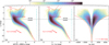 |
Fig. 2 Hess diagram of JP×Gr16.55kpc sample for a) J0378 – J0861 and b) u – i. Panel c) shows the distribution of stars in the (r vs zGC) plane. The stellar colours and magnitudes are corrected by the effect of dust (Green et al. 2018; Schlafly & Finkbeiner 2011). The horizontal dotted line indicates the absolute r magnitude equal to 4.2 mag, separating the regions we used to extract the information of ages and metallicities. The arrow illustrates the dimming and reddening vector corresponding to AV = 1 mag. The crosses arranged vertically show the colour and magnitude average errors, computed for all star within interval of size ∆r = 1 mag. |
Variables entering our hierarchical model.
3.2 stellar evolution model
We employed two stellar evolution libraries that incorporate the J-PLUS photometric system. First, the BaSTI-IAC stellar evolution models provide updated sets of solar-scaled (Hidalgo et al. 2018) and α-enhanced (Pietrinferni et al. 2021) evolutionary tracks, covering [Fe/H]from −3.20 to +0.45 dex and −3.20 to +0.06 dex, respectively, and spanning stellar masses from 0.1 to 15 M⊙. The mass step depends on the stellar mass, ranging from ∆M = 0.05 M⊙ to 1 M⊙, while the metallicity step varies from ∆[Fe/H] = 0.08 dex to 0.7 dex for solar-scaled models, and from ∆[Fe/H] = 0.15-0.20 dex for α-enhanced models. Both grids include isochrones for ages ranging from 20 Myr up to 14.5 Gyr. The solar-scaled models adopt the elemental metal distribution from Caffau et al. (2011). For the alpha-enhanced models, while the non-α elements are maintained as Caffau’s mixture, the α-elements O, Ne, Mg, Si, S, Ca, and Ti are uniformly enhanced with respect to Fe by a fixed ratio of [α/Fe]=0.4, increasing the the total metallicity [M/H] at a given [Fe/H]. Although their evolutionary tracks follow similar trends, notable differences appear in their photometry. In particular, isochrones with α enhancement tend to be slightly bluer in the B-V colour by about 0.04 mag compared to their solar-scaled counterparts, especially in the blue and ultraviolet passbands, whereas differences in the infrared and V - I colour-magnitude diagrams are less significant. This effect can also be observed in the J-PLUS photometric system, where filters bluer than 5000 Â show the largest differences in flux, making them highly sensitive to α-abundance variations (see Fig. 3). The BaSTI-IAC models account for diffusive processes, core convective overshooting, and mass loss (Reimers’ parameter ηReimers = 0.3).
The second library is PARSEC1.2S (Bressan et al. 2012; Tang et al. 2014; Chen et al. 2015), which is accessed through its public web interface5. This version assumes solar chemical mixture and provides stellar evolutionary tracks covering a wide metallicity range (−2.2 ≤ [M/H] ≤ +0.5) and initial masses from 0.1 up to 150 M⊙, with extensions reaching 350 M⊙ for subsolar metallicities ([M/H] ≤ 0.15 dex). The models include key physical processes such as microscopic diffusion, convective core overshooting, and mass loss following the Reimers formulation with an efficiency parameter of η = 0.3. Isochrones derived from these tracks are computed from the pre-MS up to advanced evolutionary phases.
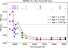 |
Fig. 3 J-PLUS magnitude differences between solar-scaled and α-enhanced BaSTI models for MSTO stars. We selected three stellar pairs at [M/H] = −0.1 dex, with approximate ages of 2.5, 5.0, and 10 Gyr and corresponding masses of 1.3, 1.1, and 1.0 M⊙, respectively. The horizontal dashed line indicates the upper limit of the median absolutemagnitude error, as averaged from the third column of Table 1. |
3.3 Sampling the CAMD
Stars in a CAMD are arranged according to intrinsic properties such as effective temperature, surface gravity, age, and chemical composition. Certain regions in the CAMD are particularly sensitive to these parameters, whereas others are not. This requires a well-sampled CAMD to maximise the information extracted from evolutionary phases that are most sensitive to the SFH.
Panels a and c in Fig. 4 illustrate how isochrones of different ages and metallicities are distributed in the CAMD. Regions covering the MSTO and the more evolved phases of stellar evolution are those containing the most information about the age of the stars, but they are subject to a strong age-metallicity degeneracy. In contrast, the low-mass MS phase is notably insensitive to age but not to metallicity. To exploit this difference, we split the CAMD at r = 4.2 mag: the upper region (r ≤ 4.2 mag) is used to derive the SFH, while the lower region (r > 4.2 mag) supplies a metallicity prior that helps mitigate possible age-metallicity degeneracies in the upper portion of the diagram.
Before assembling our isochrone grids, we assessed the minimum metallicity and age that can be reliably distinguished given our magnitude uncertainties (see Table 1). Specifically, we defined an isochrone separation ∆ Jk as the average difference in absolute Jk magnitude between two isochrones sharing the same age (or metallicity) but adjacent metallicities (or ages). This approach is illustrated in Fig. 4: for example, the doubleheaded arrow in panel b marks the r separation at (J0378 -J0861) = 1.7 mag around the MSTO and SGB phases. In panel d, we measure a similar separation at (J0378 - J0861) = 3.0 mag, computed for r ≥ 4.2 mag and stellar masses > 0.2 M⊙. Our isochrone sets must satisfy ∆Jk >, which is the average absolute magnitude error (≈0.12 mag), ensuring that any differences recovered in the posterior distribution of ai reflect actual variations in the CAMD rather than noise.
Our final set of models comprises grids from both BaSTI-IAC (for α = 0 and α = 0.4) and PARSEC, spanning ages from ~13.5 Gyr to 500 Myr in logarithmic steps, and metallicities in the −1.5 ≤ [M/H] ≤ 0.3 range. For consistency with our observations, we excluded helium burning (HB) and the asymptotic giant branch (AGB) because they are out of our completeness interval, and we limited our analysis to MS, SGB, and red giant branch (RGB) stars. Additionally, we removed pre-MS stars and adopted ηReimers = 0.3 to quantify mass loss on the RGB. Table 3 summarizes all the grids used in this work.
Another important factor is the isochrone tolerance, σ, which defines the width of the probability distribution for each isochrone’s location in the CAMD. Although a non-zero σ can improve numerical stability in cases of very small photometric errors, our absolute magnitude uncertainties (dominated by distance modulus errors) are ≈0.12 mag for all J-PLUS filters, making the effect of σ negligible (σki ≪ ∆ Jk). Hence, the choice of σ does not significantly influence the final SFH solutions in this study.
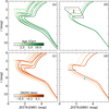 |
Fig. 4 Illustrative isochrone plot. Panel a displays a grid of nine isochrones with ages of 2.5, 5, and 10 Gyr and metallicities of [M/H] = −0.5, −0.2, and 0.1 dex. Isochrones with the same age are shown in green tones, illustrating the sensitivity of age and metallicity at the MSTO and the RGB phases. Panel b highlights the region of the CAMD where age sensitivity is highest (dashed polygon) using three isochrones of the same metallicity ([M/H] = −0.2 dex). The double-headed red arrow indicates the magnitude separation used to quantify the average distance between isochrones. Panel c shows the same grid as (a), but with orange tones indicating isochrones of the same metallicity. Panel d shows three isochrones of the same age (5 Gyr), illustrating how magnitude and colour vary with metallicity. The cyan arrow indicates the magnitude separation used to define the average distance between isochrones. |
Isochrone Grids used in this work. The step in metallicity is ∆[M/H] = 0.1 dex for all the grids.
3.4 Mitigating degeneracies with multi-filter photometry
J-PLUS photometry has demonstrated significant potential in mitigating the age-metallicity degeneracy commonly encountered in CAMD fitting. The use of multiple narrow and broad filters, strategically designed to target crucial stellar absorption features, enhances its sensitivity to elemental abundances (Cenarro et al. 2019). Specifically, filters such as u, z, J0378, and J0861 broaden the spectral baseline, thereby diminishing degeneracies between colour (or effective temperature) and metallicity and resulting in more precise determinations of [Fe/H]. Additionally, the J0395 filter, centred on the Ca IIH and K lines, strongly correlates with iron abundance, increasing the robustness of metal-licity measurements. As described in Section 3, stars fainter than the MSTO (r > 4.2 mag) are particularly effective in tracing the metallicity distribution within the JP×Gr16.55kpc sample, enabling the construction of an age-independent metallicity prior. This prior significantly reduces degeneracies for brighter stars (r ≤ 4.2 mag). Grid A in Table 3 was defined to fully exploit these properties.
The chemical sensitivity provided by the J-PLUS photometric system, in conjunction with α-enhanced isochrones, allows for consistent CAMD fitting of stellar populations with enhanced α-abundances. Filters such as J0515, centred on the Mg b triplet, and J0861, which covers the Ca II triplet (Cenarro et al. 2019), serve as indicators of magnesium and calcium relative to iron, making them useful for constraining α-element abundances. Additional filters sampling the G band (J0430) and the hydrogen Balmer lines (u) further enable J-PLUS to accurately constrain stellar atmospheric parameters and key abundance ratios, including [Mg/Fe] and [α/Fe], as evidenced by prior studies (Whitten et al. 2019; Yang et al. 2022; Huang et al. 2024). The α-enhanced BaSTI models assume a uniform enhancement pattern of [α/Fe]= 0.4 dex across elements O, Ne, Mg, Si, S, Ca, and Ti (Pietrinferni et al. 2021). Notably, the J-PLUS blue filters (< 5000Â) exhibit sensitivity to variations in α-enhancement levels within isochrones (Sect. 3.2), enabling the effective separation of high-α and low-α populations in the CAMD. The agreement between the sensitivity of J-PLUS photometry and theoretical stellar evolution models to different α-element compositions, validates the application of isochrone grids for studying α-enhanced populations, such as those found in the Galactic thick disc.
3.5 Estimating uncertainties
Grids B, C, and D span a broader range of ages and metal-licities, increasing the risk of obtaining biased SFHs due to age-metallicity degeneracies. To evaluate the impact of random uncertainties and degeneracies on the age and metallicity distributions, we performed recovery tests over a synthetic grid of simple stellar populations (SSPs). This synthetic population includes realistic photometric and parallax uncertainties characteristic of the JxG5 sample (see Appendix C).
These tests showed that the uncertainty distribution depends significantly on the SSP age and metallicity, clearly revealing the effect of parameter degeneracies. By fitting Normal and Cauchy distribution functions to the marginal distributions of [M/H] and age, we estimate typical uncertainties of σ[M/H] ≈ 0.10-0.14 dex, and σage ≈ 0.15 Gyr for young/intermediate ages and σage ≈ 0.55-1.2 Gyr for old ages, associated the JP×Gr16.55kpc sample.
These uncertainties are in good agreement with the typical values obtained by Huang et al. (2024), which reported metallic-ity uncertainties of 0.10-0.20 dex using kernel-based regression applied to J-PLUS/Gaia colours, and 20% uncertainties for stellar ages determined from isochrone fitting of MSTO and SGB stars. We did not perform a similar uncertainty estimation for α-abundance determinations, given our model’s limitation to discrete values of [α/Fe]=0.0 and 0.4 dex.
4 Results
4.1 Metallicity distribution of the MS low-mass stars
Using Grid A in Table 3, we derived the metallicity distribution for the JP×Gr16.55kpc stars that are fainter than r = 4.2 mag. Grid A contains 57 isochrones organised into three age bins (~2, 5, and 10 Gyr), with each bin containing 19 metallicity steps. We limited the ages to these three values because the faint part of the CAMD (r > 4.2 mag) is insensitive to age changes (see the top left panel of Fig. 4). Fig. 5 shows the resulting metallicity distribution. It peaks at [M/H]~ −0.2 dex, and 90% of the stars lie between −1.0 and 0.4 dex.
In contrast to the metallicity distributions obtained from APOGEE DR17, the result reveals that fits based on the PARSEC isochrones produce a reasonable distribution but tend to recover metallicities that are ~0.1 dex lower than spectroscopic values. Possible explanations for this 0.1 mag shift include underestimated extinction values from BAYESTAR and/or the possibility that the PARSEC models predict slightly cooler effective temperatures for low-mass MS stars. The 1% accuracy of the J-PLUS photometric calibration is unlikely to account for a shift of 0.1 mag (López-Sanjuan et al. 2024).
Compared to the BaSTI solar-scaled models, the PARSEC 1.2S models proved more effective at fitting the low-MS stars’ photometry of the JP×Gr16.55kpc. This may be attributed to the temperature-optical depth (T-τ) relations from PHOENIX BT-Settl atmospheres, as implemented by Chen et al. (2014). In contrast, the BaSTI models for low-mass stars are significantly bluer than the J-PLUS colours and did not yield a metallicity distribution with well-defined features. For this reason, they were not used to define the prior. A similar offset was found for the PARSEC set by Gallart et al. (2024) using Gaia data, but not for the BaSTI tracks.
On the other hand, from test analyses conducted on the bright part (r ≤ 4.2 mag) of the JP×Gr16.55kpc sample, we found that the obtained metallicity distribution is systematically biased towards higher metallicities compared to those reported by spectroscopic surveys. This effect can be observed in Gallart et al. (2024) as well, and it can be produced by the inherent age-metallicity degeneracy of the isochrones, the presence of unresolved binary stars, or even limitations in the stellar evolutionary models.
Because the metallicity distribution in the lower CAMD is essentially age-independent, we used it to define informative priors that help to mitigate the age-metallicity degeneracy when modelling the upper CAMD:
![Mathematical equation: \text{PARSEC:}\quad & [{\rm M/H}] \sim \mathcal{N}(-0.2,\,0.21)\;\text{dex}, \label{eq:prior_parsec}\\](/articles/aa/full_html/2026/02/aa57023-25/aa57023-25-eq12.png) (3)
(3)
![Mathematical equation: \text{BaSTI:}\quad & [{\rm M/H}] \sim \mathcal{N}(-0.1,\,0.21)\;\text{dex}, \label{eq:prior_basti}](/articles/aa/full_html/2026/02/aa57023-25/aa57023-25-eq13.png) (4)
(4)
where the BaSTI prior adopts the same dispersion, but is shifted by +0.10 dex, following the offset found in Fig. 5 for the metal-licity distributions between the spectroscopic data and our result. Imposing these priors during the inference process suppresses spurious high-metallicity solutions and yields more reliable age determination.
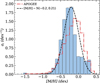 |
Fig. 5 Inferred metallicity distribution of JP×Gr16.55kpc sample (solid histogram) for stars with absolute r magnitudes fainter than 4.2 mag, using Grid A from Table 3. The dash-dotted line shows the metallicity distribution of an APOGEE DR17 sample, selected as described in Appendix A.2. The dashed line indicates the normal function adopted as the prior on [M/H] for the PARSEC models. |
4.2 Star formation history: Solar-scaled and α-enhanced models
Figures 6 and 7 show the inferred SFHs for the JP×Gr16.55kpc kpc sample (Mr ≤ 4.2 mag), obtained using grids B, C, and D from Table 3. Grids B and C correspond to the SFHs inferred using PARSEC and BaSTI models with solar-scaled abundances, respectively, while Grid D represents the SFH inferred from BaSTI models with α-enhanced abundances. These two figures thus highlight the differences introduced by the adoption of different stellar evolution codes and α-enhanced models. The age axes in these figures are presented on a linear scale and the corresponding age uncertainty is approximately σage ≈ 0.15 Gyr for young/intermediate ages and σage ≈ 0.55-1.2 Gyr (Appendix C).
Figures 6, 7a and 7b reveal a stellar population exhibiting a monotonic chemical enrichment, with metallicity increasing from about [M/H] ≃ −0.6 to −0.5 dex at 12.5 Gyr up to approximately 0.0 dex by 8 Gyr. We highlight this population’s chemical signature with a dashed white line, visually corresponding to an enrichment rate of approximately 0.13 dex Gyr−1. This line serves solely as a visual guide rather than a representation of a formal fit. Within our uncertainties, this chemical enrichment trend is consistent with age-metallicity relations derived by Xiang & Rix (2022) from LAMOST, Sahlholdt et al. (2022) from GALAH, Cerqui et al. (2025) using APOGEE, and Fernández-Alvar et al. (2025) using Gaia, specifically for the thick disc stellar population. A second metallicity enrichment pattern is clearly visible in Fig. 7b; it begins at approximately [M/H] = −0.3 dex between 8 and 7 Gyr ago and reaches [M/H] ≈ 0.0 dex by around 3 Gyr. This second enrichment feature is also partially visible in Figs. 6 and 7a, though with less clarity. All our inferred SFHs indicate the presence of stars older than 7 Gyr with metallicities of [M/H] ≥ 0.0 dex.
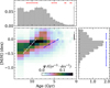 |
Fig. 6 Inferred SFH of JP×Gr16.55kpc sample for stars brighter than r = 4.2 mag, using Grid B. The grey histograms in the upper and right panels show the marginal distributions of age and metallicity, respectively. The red and blue error bars above the histograms indicate the full width at half maximum (FWHM) of the age and metallicity uncertainties, as estimated in Appendix C. The dashed and dash-dotted lines highlight the two population candidates that we consider to be detected. |
4.3 Simultaneous fitting of solar-scaled and α-enhanced models
Grid E from Table 3 includes both solar-scaled and α-enhanced isochrones. This grid allows our algorithm to determine which of the two α-abundance regimes (or combination of both) is more likely to fit the observed CAMD. In Fig. 8, we present the SFH derived from this grid, separating the distributions into the α-enhanced ([α/Fe]= 0.4 dex) and solar-scaled ([α/Fe]= 0.0 dex) components.
The marginal age distribution in Fig. 8 shows that, for the α-enhanced population, most stars formed between 12.5 and 8 Gyr ago. Conversely, marginal age distribution for the solar-scaled population, the contribution from older stars diminishes significantly, with intermediate-age populations dominating the distribution. Additionally, the SFH indicates that, for the α-enhanced population, metallicity growth slowed down at around 9 Gyr, and an intermediate-age population emerges at about 8 Gyr.
The α-enhanced SFH in Fig. 8 exhibits a chemical enrichment trend between 12.5 and 8 Gyr that closely matches those seen in Figs. 6 and 7, but with the α-enhanced models dominating over the solar-scaled ones. Metallicity growth then plateaus around 8 Gyr at [M/H] ≈ 0.1-0.2 dex, after which a second enrichment episode commences in the α-enhanced population. The apparent overlap between these two enrichment phases can be attributed to the systematic age-metallicity correlation identified in our mock tests (Appendix C).
In the solar-scaled SFH of Fig. 8, there is a significant reduction in the number of stars older than ~9-10 Gyr. Moreover, between 10 and 3 Gyr, a secondary enrichment trend is apparent, with metallicity growing more slowly compared to that of the older, high-α population. Another feature emerges at metallici-ties of [M/H] ≥ 0.0 dex, spanning ages from about 8 Gyr down to approximately 3 Gyr. This second population appears to show a slightly decreasing trend in metallicity, evolving from about (8 Gyr, 0.2 dex) down to (3 Gyr, 0.0 dex). Lastly, a third population is visible at sub-solar metallicities ([M/H] < 0.0 dex), showing a moderate increase in metallicity from approximately [M/H] = −0.4 dex between 9 and 8 Gyr ago, to about [M/H] = −0.2 dex at around 3 Gyr ago.
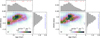 |
Fig. 7 Inferred SFH of JP×Gr16.55kpc sample for stars brighter than r = 4.2 mag, using Grid C (solar-scaled; panel a) and Grid D (α-enhanced; panel b). The grey histograms in the upper and right panels show the marginal distributions of age and metallicity, respectively. The red and blue error bars above the histograms indicate the full width at half maximum (FWHM) of the age and metallicity uncertainties, as estimated in Appendix C. The dashed and dash-dotted lines highlight the two population candidates that we consider to be detected. |
4.4 Spatially mapping metallicity and age gradients
We derived individual ages, metallicities, and [a/Fe] abundances for the JP×Gr16.55kpc stars by matching their J-PLUS photometry and Gaia parallaxes to the 1152 isochrones of Grid E. For every star, n, and isochrone, i, we computed the likelihood in Eq. (1) and adopted the parameters of the isochrone that maximised it. Apparent magnitudes and parallaxes, rather than absolute magnitudes, were fitted, ensuring internal consistency between the inferred parameters and the three-dimensional position of each star.
Figures 9, 10, and D.1 display the spatial trends of metallicity, age, and [a/Fe], respectively. Each mosaic stacks nine [M/H] (age) slices, revealing systematic variations with height above the plane and galactocentric radius. The corresponding pixel-by-pixel dispersions are presented in Figs. D.2, D.3, and D.4. Because they include the physical spread in age and metallicity along the yGC axis, these dispersions exceed the random photometric errors.
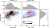 |
Fig. 8 Inferred SFH of JP×Gr16.55kpc sample for stars brighter than r = 4.2 mag, using Grid E, which simultaneously fits solar-scaled and α-enhanced isochrones (indicated as [a/Fe]=0.0 and [a/Fe]=0.4, respectively, in the panel titles). The grey histograms in the upper and right panels show the marginal distributions of age and metallicity, respectively. The red and blue error bars above the histograms represent the full width at half maximum (FWHM) of the age and metallicity uncertainties, as estimated in Appendix C. The dashed and dash-dotted lines highlight the two candidate populations that we consider to be detected. |
4.4.1 Young and intermediate-age populations (<7 Gyr)
In Fig. 9, stars younger than 7 Gyr show metallicities around 0.0 ≲ [M/H] < 0.1 dex within |zGC| ≲ 1 kpc, which increases to [M/H] ≳ 0.1 dex for |zGC| ≲ 0.75 kpc. This distribution is similar to that observed in APOGEE DR17 (Imig et al. 2023, their Fig. 5), where [Fe/H]< −0.2 for |z/kpc| < 1. A small fraction of young stars with [M/H] ≈ 0 dex reach |zGC| ≃ 1-2 kpc, and those with [M/H] ≤ −0.1 dex extend even higher. Although these heights exceed the canonical thin disc scale height of ~200 pc (e.g. Bovy 2017), similar low-[a/Fe] stars are observed at 1 ≲ |z|/kpc ≲ 2 and 6 < RGC/kpc < 9 in the APOGEE sample (Fig. 8 from Imig et al. 2023).
The mean age distribution for different metallicity bins is shown in Fig. 10. For metal-poor stars ([M/H] ≤ −0.4 dex), there is little to no age gradient, which is consistent with the uniform distribution of old, metal-poor stars from the halo and thick disc. At intermediate metallicities (−0.4 to 0.2 dex), however, we observe a mild gradient in the mean stellar age with respect to zGC. This is precisely the metallicity range where the two populations identified in Figs. 7 and 8 coexist, but with different ages.
Young stars (<6 Gyr) with −0.2 < [M/H]/dex ≤ 0.2 dominate the mean age within 1 kpc and towards the Galactic anticentre (cyan and dark green pixels), whereas older stars (6-8 Gyr) dominate at higher vertical positions (zGC > 1 kpc). Some spurious effects appear in pixels at larger heliocentric distances, especially in the high-metallicity range, where unrealistically young ages are inferred. Such ages are not consistent with expectations at those vertical positions. These effects are likely caused by the small number of stars and parallax errors at large distances, since distance affects both the derived age and the Bayestar 3D reddening-map solution. Indeed, we observe large age variance in these pixels (see Fig. D.3). In contrast, metallicity depends mainly on colour and is therefore far less sensitive to distance errors.
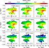 |
Fig. 9 Metallicity map in galactocentric xGC and zGC coordinates of JP×Gr16.55kpc (r ≤ 4.2 mag) sample. The metallicity values were derived as described in Sect. 4.4, using Grid E (solar+α-enhanced isochrones) from Table 3. The colour bar indicates the mean of [M/H] for stars within 0.2 × 0.2 kpc2 pixels. The pixels with fewer than ten stars were rejected. |
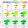 |
Fig. 10 Age map in galactocentric xGC and yGC coordinates of JP×Gr16.55kpc (r ≤ 4.2 mag) sample. The age values were derived as described in Sect. 4.4, using Grid E. The colour bar indicates the mean a for stars within 0.2 × 0.2 kpc pixels. The pixels with fewer than 10 stars were rejected. |
4.4.2 Old populations (>8 Gyr)
For ages older than 8 Gyr, stars with −0.4 ≲ [M/H]/dex ≲ -0.1 dex dominate the distribution around |zGC| ≃ 2 kpc, extending farther than their more metal-rich counterparts ([M/H] ≳ -0.1 dex). The oldest and most metal-poor stars ([M/H] ≲ -0.6 dex) lie even higher and probably belong to the thick disc, with a small fraction originating from the stellar halo. A pronounced vertical metallicity gradient appears in the 9.5 < Age/Gyr ≤ 12.6 panel, dropping from [M/H] ≃ −0.1 dex at the plane to [M/H] ≲ -0.7 dex at large |zGC|.
Figure 10 reveals no obvious age-zGC trend for the old sample, but a clear dependence on xGC : the relative number of 8-10.5 Gyr stars increases towards the Galactic centre, consistently with the stellar-density profile of the thick disc. Stars older than 10.5 Gyr dominate at [M/H] ≲ -0.6 dex and become exclusive below [M/H] ≈ −1 dex, in line with a halo origin. See Appendix D for further information about the distribution of [α/Fe] as a function of the xGC and zGC coordinates.
5 Discussion
The SFH of the JP×Gr16.55kpc shows at least two populations with different chemical evolutions. The first one, formed by α-enhanced stars born between 12.5 and 8 Gyr ago. The second one, which seems to be formed mainly by solar-scaled stars, evolved from ~8 Gyr ago to today. In this section, we discuss both populations and compare our results with those of other works.
5.1 Signatures of the Galactic thick disc formation
The age distribution of [α/Fe]=0.4 dex in Fig. 8 reveals a chemical enrichment that began at the oldest ages, from 13.7 to 11.3 Gyr ago6, and was relatively short. Approximately within ≈4.5 Gyr, the interstellar medium (ISM) was driven from [M/H] ≈ −0.5 dex to super-solar values, as the sequence ended around 8 Gyr ago. This old, high-α component of the SFH is likely linked to a significant number of thick disc stars from the same JP×Gr16.55kpc, and it can be related to a relatively short and intense formation episode. Independent large-survey studies report a similar chronology. Sahlholdt et al. (2022) showed how GALAH MSTO stars outline one narrow age-metallicity ridge that terminated about 10 Gyr ago, implying an equally intense early star-formation episode. APOGEE mapping of high-α stars finds a median age of ≲ 9 Gyr throughout the disc, again suggesting a rapid first phase despite later selection biases (Cerqui et al. 2025). The Gaia colour-magnitude analysis made by Fernández-Alvar et al. (2025) pushes the onset even earlier, to 13 Gyr, and shows enrichment to super-solar metallicity by 10 Gyr, while the dynamically selected sample of LAMOST SGB stars in Xiang & Rix (2022) trace a remarkably tight [Fe/H]-age track from −1 dex at 13 Gyr to 0.5 dex by 7-8 Gyr, implying a well-mixed ISM during the entire high-α phase.
The well-shaped enrichment trend we recovered in Fig. 8 for [α/Fe]=0.4 dex, even when observational age scatter is present, matches our expectation when a dense and well-mixed gas reservoir is consumed in a brief, intense star-formation episode. In the simulations of Khoperskov et al. (2021), this phase reached ≥10 M⊙ ∙ yr−1 for several hundred million years, producing a compact, high-α disc whose chemistry evolves almost synchronously across radius because the ISM is efficiently stirred and enriched. The Auriga simulation from Grand et al. (2018) shows that a centrally concentrated starburst, often merger-triggered, drives the ISM from [Fe/H]≈ - 0.5 dex to super-solar within ≲3 Gyr, after which point the gas disc contracts, the SFR decreases sharply, and a chemically distinct low-α sequence begins to grow from newly accreted gas. The Agertz et al. (2021) VINTERGATAN simulation links a similar transition to the Galaxy’s last major merger. While the inner high-α disc survives, the encounter seeds an extended, metal-poor and low-α outer disc, whose lower SFR mode soon dominates the posterior generation of stars. Our SFH shows a similar turning point, marked by a sharp decline in α-rich star formation after ≈9 Gyr, accompanied by a rise in solar-scaled star formation from 10 Gyr towards younger ages.
In general, major mergers can significantly affect the internal star formation of the host galaxy. For instance, simulations by Moreno et al. (2015) show that the first peri-centric passage of the less massive companion enhances star formation in the central regions of the primary galaxy. In this context, Fernández-Alvar et al. (2025) linked their 10.5 Gyr enhancement of star formation explicitly to the GSE merger. While the uncertainties in our results limit the scope of the discussion, our inferred SFHs remain consistent with a scenario in which the GSE merger contributed to shaping the early disc. This motivates extending the analysis by incorporating spatial and/or kinematical selections to explore possible hidden features in the SFHs.
The [α/Fe]=0.4 SFH in Fig. 8 shows a population of stars with [M/H] > 0 at 7-9 Gyr. Given the strong incompleteness of our JP×Gr16.55kpc (r ≤ 4.2 mag) sample below |zGC| < 400 pc, the number of inner-disc migrant stars is significantly reduced. We therefore interpret these [M/H] > 0 stars as likely representing the tail end of the early, well-mixed chemical evolution, rather than later arrivals from the inner Galactic region. Xiang & Rix (2022) reported that their high-α sequence naturally extends to 0.5 dex by 7 Gyr; it was produced in situ from a thoroughly stirred ISM rather than by radial migration.
Collectively, these studies reinforce the view that the Milky Way’s thick disc was forged during a short, intense, central burst, and that the drop in α-rich star formation around 9 Gyr ago marks the transition to the less intense, low-α regime traced by the thin disc.
5.2 Clues to the Galactic thin disc history
Our results reveal a chemically distinct stellar population for ages younger than 8 Gyr, which is characterised by a low-α abundance pattern and a slower metallicity enrichment compared to the α-enhanced population. This is consistent with the scenario of a different star formation regime, in which the ISM becomes enriched primarily through Type Ia supernovae over longer timescales. In this context, Fernández-Alvar et al. (2025) report a more gradual chemical evolution in the thin disc component of their kinematically selected sample, with a particularly modest enrichment in the SFH for stars younger than 6 Gyr.
Similarly, the low-α population analysed in Xiang & Rix (2022) displays a significantly slower chemical enrichment than its highα counterpart. The intermediate/young sequence traced by the dot-dashed blue line in Fig. 7a are in agreement with these findings, which we identify as a low-α population forming under quieter conditions and in a more chemically evolved environment than the thick disc progenitors. This sequence overlaps in time with the tail end of the α-enhanced formation period (see Fig. 7b and Fig. 8), which is inconsistent with an early coformation of the thin and thick discs (Beraldo e Silva et al. 2021). This behaviour could reflect a dilution episode in the ISM, as the solar-scaled isochrones better match the substructure below the blue track in Fig. 8 for [α/Fe]=0.0 dex, while the α-enhanced isochrones remain appropriate above it.
Such dilution patterns are naturally explained by simulations. Khoperskov et al. (2021) demonstrated that the strong feedback responsible for halting thick disc formation can drive metalrich gas out of the star-forming regions, after which the ISM becomes diluted by inflowing, metal-poor gas from the halo or outer disc. This resumes star formation at a lower rate and over longer timescales, generating a low-α population in a chemically distinct sequence. Similarly, the VINTERGATAN simulation by Agertz et al. (2021) shows that the last major merger led to a moderate mode of star formation, effectively ending the thick disc era. In their scenario, the thin disc gradually builds up from cosmological accretion and gas stripped from satellites, forming stars with lower [α/Fe] in an extended disc configuration. Although Grand et al. (2018) describe a different mechanism, a shrinking and subsequent regrowth of the gas disc from external accretion, the outcome is similar: a chemically separate, low-α sequence emerges following the peak of early star formation.
Additional evidence of radial migration may also be present in our results. In Fig. 8 for [α/Fe]=0.0 dex, we identify stars with [M/H] > 0.0 and ages older than 6 Gyr, which could be interpreted as stars born in the inner disc, after the thick disc phase, in a metal-rich but low-α environment, and later redistributed outward via secular migration. This is consistent with the timescales expected for stars to reach larger orbital radii under realistic migration rates. Finally, we note that incompleteness in our sample near the Galactic plane could hinder the detection of stars born in localized star formation events. Notably, the starburst episode linked to the passage of the Sagittarius dwarf galaxy, possibly around 5-6 Gyr ago as proposed by Ruiz-Lara et al. (2020a) and Fernández-Alvar et al. (2025), may be underrepresented in our results due to this selection limit.
6 Conclusions
We inferred the SFHs of a sample of stars located within 5 kpc and with the magnitude limits mr = 14 mag and mr = 16.5 mag. Our analysis combined trigonometric parallaxes with 12 photometric bands from the Gaia and J-PLUS DR3 catalogues, using a Bayesian CMD-parallax fitting approach. This method supports any number of filters, incorporates prior distributions on metal-licity, accounts for selection effects due to magnitude limits, and fits distance and photometry in a fully consistent framework.
The simultaneous fitting of solar-scaled and α-enhanced isochrones reveals distinct formation epochs for chemically different stellar populations in the Galactic disc. The α-enhanced component dominates the early SFH, with most stars forming between 12.5 and 8 Gyr ago. This period exhibits a well-defined chemical enrichment sequence, consistent with intense star formation driven by a dense, efficiently mixed ISM. This result is in agreement with previous observational works such as (Xiang & Rix 2022; Fernández-Alvar et al. 2025) and simulations such as those by Khoperskov et al. (2021) and Grand et al. (2018).
In contrast, the solar-scaled population is dominated by intermediate-age stars formed between 9 and 3 Gyr ago, with only a minor contribution from older stars. This population exhibits a slower chemical enrichment trend, characteristic of a lower star formation regime, with iron abundances primarily increased through Type Ia supernovae. A slightly decreasing metallicity trend is also observed at super-solar values between ages of 8 and 5 Gyr, suggesting that radial migration contributes to the present-day composition of the thin disc. The presence of multiple sub-populations, spanning both solar and sub-solar metallicities, indicates a more complex and prolonged SFH. These stars likely trace the evolutionary phases of the thin disc, shaped by extended chemical evolution driven by secular processes rather than rapid early enrichment.
The resulting maps of mean [M/H], age, and [α/Fe] across the Galactic plane reveal coherent spatial trends. For old stars (9.5 < Age/Gyr ≤ 12.6), the vertical metallicity gradient is pronounced, decreasing from [M/H] ≃ −0.1 dex near the plane to [M/H] ≲ -0.7 dex at large |zGC|. The fraction of stars with ages between 8 and 10.5 Gyr increases towards the inner disc, consistently with a thick disc density profile, while stars with [M/H] ≲ -1 dex are found to be almost exclusively older than 10.5 Gyr, as expected for a stellar halo component. In addition, stars younger than 7 Gyr are generally metal-rich and concentrated close to the plane, xhich is consistent with the expected properties of the thin disc populations.
The multi-filter photometry from J-PLUS has been instrumental in mitigating the age-metallicity and α-element degeneracies inherent to CMD fitting based on broadband photometry with a low number of filters. By incorporating strategically chosen narrow and broad filters sensitive to key stellar absorption features, we achieve a more robust characterisation of stellar metallicities and elemental abundances. This chemical sensitivity allowed us to derive an age-independent metallicity distribution, which was later incorporated into our analysis as a prior on [M/H], improving the reliability of the SFH inference across the CAMD. The combination of J-PLUS photometry, our methodology, and theoretical stellar evolution models with varying α-element compositions allows the simultaneous identification of high- and low-α populations, demonstrating the potential of J-PLUS data to constrain distinct star formation regimes and chemical enrichment histories within the Milky Way. Furthermore, the methodology presented here is well suited to exploiting large photometric datasets such as J-PAS, S-PLUS, and LSST, and is versatile enough to incorporate individual stellar metal-licities and kinematics, enabling a robust and detailed analysis of the Milky Way’s SFH across spatial, temporal, and chemical scales.
Data availability
The files containing the inferred ai values used in Figs. 6, 7, and 8, together with the catalogue containing the individual stellar ages and metallicities used in Figs. 9, 10 and D.1, are available at Zenodo (DOI: 10.5281/zenodo.17592911).
Acknowledgements
J.A.A.T. acknowledges the financial support from the European Union - NextGenerationEU through the Recovery and Resilience Facility (RRF) program Planes Complementarios con las CCAA de Astrofísica y Física de Altas Energías - LA4. A.E. acknowledges the financial support from the Spanish Ministry of Science and Innovation and the European Union - NextGenerationEU through the RRF project ICTS-MRR-2021-03-CEFCA. A. H. acknowledges the financial support of the Spanish Ministry of Science and Innovation (MCIN/AEI/10.13039/501100011033) and FEDER, A way of making Europe with grant PID2021-124918NB-C41 A. del Pino acknowledges financial support from the Severo Ochoa grant CEX2021-001131-S (MICIU/AEI/10.13039/501100011033), the Ramón y Cajal fellowship RYC2022-038448-I (MICIU/AEI/10.13039/501100011033, co-funded by the European Social Fund Plus), and the RyC-MAX grant 20245MAX008 (CSIC). Based on observations made with the JAST80 telescope and T80Cam camera for the J-PLUS project at the Observatorio Astrofísico de Javalambre (OAJ), in Teruel, owned, managed, and operated by the Centro de Estudios de Física del Cosmos de Aragón (CEFCA). We acknowledge the OAJ Data Processing and Archiving Unit (UPAD; Cristóbal-Hornillos et al. 2012) for reducing the OAJ data used in this work. Funding for the J-PLUS Project has been provided by the Governments of Spain and Aragón through the Fondo de Inversiones de Teruel; the Aragonese Government through the Research Groups E96, E103, E16_17R, E16_20R, and E16_23R; the Spanish Ministry of Science and Innovation (MCIN/AEI/10.13039/501100011033 y FEDER, Una manera de hacer Europa) with grants PID2021-124918NB-C41, PID2021-124918NB-C42, PID2021-124918NA-C43, and PID2021-124918NB-C44; the Spanish Ministry of Science, Innovation and Universities (MCIU/AEI/FEDER, UE) with grants PGC2018-097585-B-C21 and PGC2018-097585-B-C22; the Spanish Ministry of Economy and Competitiveness (MINECO) under AYA2015-66211-C2-1-P, AYA2015-66211-C2-2, AYA2012-30789, and ICTS-2009-14; and European FEDER funding (FCDD10-4E-867, FCDD13-4E-2685). The Brazilian agencies FINEP, FAPESP, and the National Observatory of Brazil have also contributed to this Project. This work presents results from the European Space Agency (ESA) space mission Gaia. Gaia data are being processed by the Gaia Data Processing and Analysis Consortium (DPAC). Funding for the DPAC is provided by national institutions, in particular the institutions participating in the Gaia MultiLateral Agreement (MLA). The Gaia mission website is https://www.cosmos.esa.int/gaia. The Gaia archive website is https://archives.esac.esa.int/gaia. This research has partially funded by MICI-U/AEI/10.13039/501100011033/ through grant PID2023-146210NB-I00. AAC acknowledges financial support from the Severo Ochoa grant CEX2021-001131-S funded by MCIN/AEI/10.13039/501100011033 and the project PID2023-153123NB-I00 funded by MCIN/AEI. L.L.N. thanks Fundaçâo de Amparo à Pesquisa do Estado do Rio de Janeiro (FAPERJ) for granting the postdoctoral research fellowship E-40/2021(280692). The work of V.M.P. is supported by NOIRLab, which is managed by the Association of Universities for Research in Astronomy (AURA) under a cooperative agreement with the U.S. National Science Foundation.
References
- Agertz, O., Renaud, F., Feltzing, S., et al. 2021, MNRAS, 503, 5826 [NASA ADS] [CrossRef] [Google Scholar]
- Alzate, J. A., Bruzual, G., & Díaz-González, D. J. 2021, MNRAS, 501, 302 [Google Scholar]
- Aparicio, A., & Gallart, C. 2004, AJ, 128, 1465 [NASA ADS] [CrossRef] [Google Scholar]
- Bailer-Jones, C. A. L. 2015, PASP, 127, 994 [Google Scholar]
- Belokurov, V., Erkal, D., Evans, N. W., Koposov, S. E., & Deason, A. J. 2018, MNRAS, 478, 611 [Google Scholar]
- Beraldo e Silva, L., Debattista, V. P., Nidever, D., Amarante, J. A. S., & Garver, B. 2021, MNRAS, 502, 260 [NASA ADS] [CrossRef] [Google Scholar]
- Bernard, E. J. 2018, in IAU Symposium, 334, Rediscovering Our Galaxy, eds. C. Chiappini, I. Minchev, E. Starkenburg, & M. Valentini, 158 [Google Scholar]
- Bland-Hawthorn, J., & Gerhard, O. 2016, ARA&A, 54, 529 [Google Scholar]
- Bonoli, S., Marín-Franch, A., Varela, J., et al. 2021, A&A, 653, A31 [NASA ADS] [CrossRef] [EDP Sciences] [Google Scholar]
- Borucki, W. J., Koch, D., Basri, G., et al. 2010, Science, 327, 977 [Google Scholar]
- Bovy, J. 2017, MNRAS, 470, 1360 [NASA ADS] [CrossRef] [Google Scholar]
- Bressan, A., Marigo, P., Girardi, L., et al. 2012, MNRAS, 427, 127 [NASA ADS] [CrossRef] [Google Scholar]
- Brown, A. G. A. 2021, ARA&A, 59, 59 [Google Scholar]
- Buder, S., Sharma, S., Kos, J., et al. 2021, MNRAS, 506, 150 [NASA ADS] [CrossRef] [Google Scholar]
- Caffau, E., Ludwig, H.-G., Steffen, M., et al. 2011, Sol. Phys., 268, 255 [NASA ADS] [CrossRef] [Google Scholar]
- Cardelli, J. A., Clayton, G. C., & Mathis, J. S. 1989, ApJ, 345, 245 [Google Scholar]
- Cenarro, A. J., Moles, M., Marín-Franch, A., et al. 2014, Proc. SPIE, 9149, 91491I [Google Scholar]
- Cenarro, A. J., Moles, M., Cristóbal-Hornillos, D., et al. 2019, A&A, 622, A176 [NASA ADS] [CrossRef] [EDP Sciences] [Google Scholar]
- Cerqui, V., Haywood, M., Snaith, O., Di Matteo, P., & Casamiquela, L. 2025, A&A, 699, A277 [NASA ADS] [CrossRef] [EDP Sciences] [Google Scholar]
- Chaplin, W. J., Serenelli, A. M., Miglio, A., et al. 2020, Nat. Astron., 4, 382 [Google Scholar]
- Chen, Y., Girardi, L., Bressan, A., et al. 2014, MNRAS, 444, 2525 [Google Scholar]
- Chen, Y., Bressan, A., Girardi, L., et al. 2015, MNRAS, 452, 1068 [Google Scholar]
- Cole, A. A., Skillman, E. D., Tolstoy, E., et al. 2007, ApJ, 659, L17 [Google Scholar]
- Cooper, A. P., Koposov, S. E., Allende Prieto, C., et al. 2023, ApJ, 947, 37 [NASA ADS] [CrossRef] [Google Scholar]
- Cristóbal-Hornillos, D., Gruel, N., Varela, J., et al. 2012, SPIE CS, 8451 [Google Scholar]
- Dal Tio, P., Mazzi, A., Girardi, L., et al. 2021, MNRAS, 506, 5681 [NASA ADS] [CrossRef] [Google Scholar]
- Dalton, G., Trager, S., Abrams, D. C., et al. 2016, SPIE Conf. Ser., 9908, 99081G [Google Scholar]
- de Jong, R. S., Agertz, O., Berbel, A. A., et al. 2019, The Messenger, 175, 3 [NASA ADS] [Google Scholar]
- De Silva, G. M., Freeman, K. C., Bland-Hawthorn, J., et al. 2015, MNRAS, 449, 2604 [NASA ADS] [CrossRef] [Google Scholar]
- del Pino, A., Hidalgo, S. L., Aparicio, A., et al. 2013, MNRAS, 433, 1505 [Google Scholar]
- del Pino, A., Łokas, E. L., Hidalgo, S. L., & Fouquet, S. 2017, MNRAS, 469, 4999 [Google Scholar]
- del Pino, A., López-Sanjuan, C., Hernán-Caballero, A., et al. 2024, A&A, 691, A221 [NASA ADS] [CrossRef] [EDP Sciences] [Google Scholar]
- Dolphin, A. E. 2002, MNRAS, 332, 91 [NASA ADS] [CrossRef] [Google Scholar]
- Fernández-Alvar, E., Ruiz-Lara, T., Gallart, C., et al. 2025, A&A, 704, A258 [NASA ADS] [CrossRef] [EDP Sciences] [Google Scholar]
- Foreman-Mackey, D., Hogg, D. W., Lang, D., & Goodman, J. 2013, PASP, 125, 306 [Google Scholar]
- Gaia Collaboration (Prusti, T., et al.) 2016, A&A, 595, A1 [NASA ADS] [CrossRef] [EDP Sciences] [Google Scholar]
- Gaia Collaboration (Brown, A. G. A., et al.) 2018, A&A, 616, A1 [NASA ADS] [CrossRef] [EDP Sciences] [Google Scholar]
- Gaia Collaboration (Smart, R. L., et al.) 2021, A&A, 649, A6 [EDP Sciences] [Google Scholar]
- Gaia Collaboration (Vallenari, A., et al.) 2023, A&A, 674, A1 [NASA ADS] [CrossRef] [EDP Sciences] [Google Scholar]
- Gallart, C., Freedman, W. L., Aparicio, A., Bertelli, G., & Chiosi, C. 1999, AJ, 118, 2245 [NASA ADS] [CrossRef] [Google Scholar]
- Gallart, C., Bernard, E. J., Brook, C. B., et al. 2019, Nat. Astron., 3, 932 [NASA ADS] [CrossRef] [Google Scholar]
- Gallart, C., Surot, F., Cassisi, S., et al. 2024, A&A, 687, A168 [NASA ADS] [CrossRef] [EDP Sciences] [Google Scholar]
- Gelman, A., Carlin, J., Stern, H., et al. 2013, Bayesian Data Analysis, 3rd Edn., Chapman & Hall/CRC Texts in Statistical Science (Taylor & Francis) [Google Scholar]
- González-Koda, Y. K., Ruiz-Lara, T., Gallart, C., et al. 2025, A&A, 704, A259 [NASA ADS] [CrossRef] [EDP Sciences] [Google Scholar]
- Grand, R. J. J., Bustamante, S., Gómez, F. A., et al. 2018, MNRAS, 474, 3629 [NASA ADS] [CrossRef] [Google Scholar]
- Green, G. M., Schlafly, E. F., Finkbeiner, D. P., et al. 2015, ApJ, 810, 25 [Google Scholar]
- Green, G. M., Schlafly, E. F., Finkbeiner, D., et al. 2018, MNRAS, 478, 651 [Google Scholar]
- Grossmann, D. H., Beck, P. G., Mathur, S., et al. 2025, A&A, 696, A42 [NASA ADS] [CrossRef] [EDP Sciences] [Google Scholar]
- Helmi, A., Babusiaux, C., Koppelman, H. H., et al. 2018, Nature, 563, 85 [Google Scholar]
- Hidalgo, S. L., Aparicio, A., Martinez-Delgado, D., & Gallart, C. 2009, ApJ, 705, 704 [Google Scholar]
- Hidalgo, S. L., Pietrinferni, A., Cassisi, S., et al. 2018, ApJ, 856, 125 [Google Scholar]
- Howell, S. B., Sobeck, C., Haas, M., et al. 2014, PASP, 126, 398 [Google Scholar]
- Huang, Y., Beers, T. C., Xiao, K., et al. 2024, ApJ, 974, 192 [Google Scholar]
- Imig, J., Price, C., Holtzman, J. A., et al. 2023, ApJ, 954, 124 [CrossRef] [Google Scholar]
- Ivezic, Z., Kahn, S. M., Tyson, J. A., et al. 2019, ApJ, 873, 111 [NASA ADS] [CrossRef] [Google Scholar]
- Jin, S., Trager, S. C., Dalton, G. B., et al. 2024, MNRAS, 530, 2688 [NASA ADS] [CrossRef] [Google Scholar]
- Khoperskov, S., Haywood, M., Snaith, O., et al. 2021, MNRAS, 501, 5176 [NASA ADS] [CrossRef] [Google Scholar]
- Kim, B., Koposov, S. E., Li, T. S., et al. 2025, MNRAS, 540, 264 [Google Scholar]
- Kordopatis, G., Schultheis, M., McMillan, P. J., et al. 2023, A&A, 669, A104 [NASA ADS] [CrossRef] [EDP Sciences] [Google Scholar]
- Kroupa, P. 2001, MNRAS, 322, 231 [NASA ADS] [CrossRef] [Google Scholar]
- Lian, J., Thomas, D., Maraston, C., et al. 2020, MNRAS, 497, 2371 [Google Scholar]
- López-Sanjuan, C., Vázquez Ramió, H., Xiao, K., et al. 2024, A&A, 683, A29 [NASA ADS] [CrossRef] [EDP Sciences] [Google Scholar]
- Luo, A. L., Zhao, Y.-H., Zhao, G., et al. 2015, Res. Astron. Astrophys., 15, 1095 [Google Scholar]
- Majewski, S. R., Schiavon, R. P., Frinchaboy, P. M., et al. 2017, AJ, 154, 94 [NASA ADS] [CrossRef] [Google Scholar]
- Marin-Franch, A., Taylor, K., Cenarro, J., Cristobal-Hornillos, D., & Moles, M. 2015, in IAU General Assembly, 29, 2257381 [Google Scholar]
- Mathur, S., Metcalfe, T. S., Woitaszek, M., et al. 2012, ApJ, 749, 152 [NASA ADS] [CrossRef] [Google Scholar]
- Mazzi, A., Girardi, L., Trabucchi, M., et al. 2024, MNRAS, 527, 583 [Google Scholar]
- Mendes de Oliveira, C., Ribeiro, T., Schoenell, W., et al. 2019, MNRAS, 489, 241 [NASA ADS] [CrossRef] [Google Scholar]
- Monelli, M., Hidalgo, S. L., Stetson, P. B., et al. 2010, ApJ, 720, 1225 [CrossRef] [Google Scholar]
- Moreno, J., Torrey, P., Ellison, S. L., et al. 2015, MNRAS, 448, 1107 [NASA ADS] [CrossRef] [Google Scholar]
- Pietrinferni, A., Hidalgo, S., Cassisi, S., et al. 2021, ApJ, 908, 102 [NASA ADS] [CrossRef] [Google Scholar]
- Queiroz, A. B. A., Anders, F., Chiappini, C., et al. 2023, A&A, 673, A155 [NASA ADS] [CrossRef] [EDP Sciences] [Google Scholar]
- Ricker, G. R., Winn, J. N., Vanderspek, R., et al. 2015, J. Astron. Telesc. Instrum. Syst., 1, 014003 [Google Scholar]
- Ruiz-Lara, T., Gallart, C., Bernard, E. J., & Cassisi, S. 2020a, Nat. Astron., 4, 965 [NASA ADS] [CrossRef] [Google Scholar]
- Ruiz-Lara, T., Gallart, C., Monelli, M., et al. 2020b, A&A, 639, L3 [EDP Sciences] [Google Scholar]
- Sahlholdt, C. L., Feltzing, S., & Feuillet, D. K. 2022, MNRAS, 510, 4669 [NASA ADS] [CrossRef] [Google Scholar]
- Savino, A., Koch, A., Prudil, Z., Kunder, A., & Smolec, R. 2020, A&A, 641, A96 [NASA ADS] [CrossRef] [EDP Sciences] [Google Scholar]
- Schlafly, E. F., & Finkbeiner, D. P. 2011, ApJ, 737, 103 [Google Scholar]
- Sharma, S., Stello, D., Bland-Hawthorn, J., et al. 2019, MNRAS, 490, 5335 [NASA ADS] [CrossRef] [Google Scholar]
- Small, E. E., Bersier, D., & Salaris, M. 2013, MNRAS, 428, 763 [Google Scholar]
- Soderblom, D. R. 2010, ARA&A, 48, 581 [Google Scholar]
- Steinmetz, M., Guiglion, G., McMillan, P. J., et al. 2020a, AJ, 160, 83 [NASA ADS] [CrossRef] [Google Scholar]
- Steinmetz, M., Matijevic, G., Enke, H., et al. 2020b, AJ, 160, 82 [NASA ADS] [CrossRef] [Google Scholar]
- Tang, J., Bressan, A., Rosenfield, P., et al. 2014, MNRAS, 445, 4287 [NASA ADS] [CrossRef] [Google Scholar]
- Tosi, M., Greggio, L., Marconi, G., & Focardi, P. 1991, AJ, 102, 951 [NASA ADS] [CrossRef] [Google Scholar]
- Walmswell, J. J., Eldridge, J. J., Brewer, B. J., & Tout, C. A. 2013, MNRAS, 435, 2171 [Google Scholar]
- Weisz, D. R., Dolphin, A. E., Skillman, E. D., et al. 2014, ApJ, 789, 148 [NASA ADS] [CrossRef] [Google Scholar]
- Whitten, D. D., Placco, V. M., Beers, T. C., et al. 2019, A&A, 622, A182 [NASA ADS] [CrossRef] [EDP Sciences] [Google Scholar]
- Xiang, M., & Rix, H.-W. 2022, Nature, 603, 599 [NASA ADS] [CrossRef] [Google Scholar]
- Yan, H., Li, H., Wang, S., et al. 2022, The Innovation, 3, 100224 [NASA ADS] [CrossRef] [Google Scholar]
- Yang, L., Yuan, H., Xiang, M., et al. 2022, A&A, 659, A181 [NASA ADS] [CrossRef] [EDP Sciences] [Google Scholar]
- Yanny, B., Rockosi, C., Newberg, H. J., et al. 2009, AJ, 137, 4377 [Google Scholar]
All the J-PLUS DR3 catalogues are available at https://archive.cefca.es/catalogues/jplus-dr3/help_adql.html
For simplicity, and hereafter, we denote the absolute r magnitude in the CAMD simply as r.
In isochrone grids B, C, D, and E, the oldest age is ≈12.5 Gyr and covers the interval ranging from 13.7 to 11.3 Gyr.
Appendix A Data Queries and Sample Definitions
Appendix A.1 J-PLUS filter set and data query
Table A.1 shows the basic characteristics of the J-PLUS passbands. The first column (k) denotes the index number assigned to each filter. In Section 3.1, we define the absolute Jk magnitude, where each component (J1, J2, ..., J12) corresponds to the filters listed in this table. This indexing facilitates the reference and manipulation of filter-specific data within our analysis.
J-PLUS filter set.
To ensure the reliability of our photometric measurements, we selected sources using the following quality criteria: (i) the maximum SExtractor FLAGS value across all filters is less than 3, permitting only minor detection issues (e.g., proximity to bright neighbours or image borders), except for sources in the mr band where we additionally allow FLAGS values between 2048 and 2051 to include forced photometry cases; (ii) the maximum MASK_FLAGS value is less than 1, thereby excluding sources affected by masked or defective pixels; and (iii) the minimum normalised weight map value (NORM_WMAP_VAL) across all filters exceeds 0.8, ensuring high data quality in all bands. These criteria collectively provide a robust sample for our study of the Galactic disc.
We applied the 2σ confidence interval criteria from del Pino et al. (2024) to achieve a purer sample of stars by imposing hard constraints on the probabilities of an object belonging to each of the three classified categories: Galaxy, QSO, or Star. Specifically, for an object to be classified as a star at the 2σ confidence level, the 98th percentile of its probability of being a galaxy (PCGalaxy(98)) and the 98th percentile of its probability of being a QSO (PCQSO(98)) must both be less than 1/3. Simultaneously, the 2nd percentile of its probability of being a star (PCStar(02)) must be greater than 1/3. This approach results in a highly confident stellar sample, though it may lead to a reduction in the sample’s overall completeness compared to less stringent criteria
SELECT
- - Columns --
MagAB.TILE_ID,
MagAB.NUMBER,
MagAB_F.ALPHA_J2000, MagAB_F.DELTA_J2000, MagAB.MAG_APER_COR_3_0, MagAB_F.MAG_ERR_APER_3_0,
FROM jplus.MagABDualPointSources AS MagAB
- - Join with other catalogs -
LEFT JOIN jplus.MagABDualObj AS MagAB_F ON ((MagAB.NUMBER = MagAB_F.NUMBER) AND (MagAB.TILE_ID = MagAB_F.TILE_ID))
LEFT JOIN jplus.ClassBANNJOS AS BANNJOS ON ((MagAB.NUMBER = BANNJOS.NUMBER) AND (MagAB.TILE_ID = BANNJOS.TILE_ID))
WHERE
- - Good photometry --
(ARRAY_MAX_INT(MagAB_F.FLAGS)<3 OR
MagAB_F.FLAGS[jplus::rSDSS] BETWEEN 2048 AND 2051)
AND ARRAY_MAX_INT(MagAB_F.MASK_FLAGS)<1
AND ARRAY_MIN_FLOAT(MagAB_F.NORM_WMAP_VAL)>0.8
- - BANNJOS classification -
AND ( (BANNJOS.CLASS_STAR_prob_pc02 >= 0.333)
AND (BANNJOS.CLASS_QSO_prob_pc98 < 0.333)
AND (BANNJOS.CLASS_GALAXY_prob_pc98 < 0.333) )
AND (MagAB.MAG_APER_COR_3_0[1] BETWEEN 14. AND 19.)
Appendix A.2 APOGEE sample selection
To ensure a high-quality and reliable sample from the APOGEE DR17 catalog, we selected stars with SNR ≥ 70 to guarantee precise stellar parameter and abundance determinations. We required stars to have Simple. Additionally, we required STARFLAG= 0, retained only those stars for which FE_H_FLAG= 0 and ϖ ≥ 0.2 mas.
Appendix B Detailed formulations of our Bayesian model
This appendix presents the detailed mathematical formulations that built the Bayesian inference framework employed in this study. In Appendix B.1, we describe the selection and structure of the prior distributions and likelihood functions, providing an explanation of the assumptions and reasoning behind these choices. Appendix B.2 then derives the marginal posterior distribution, explicitly incorporating a data completeness function to correct for potential biases in the observed sample. See Table 2 to identify all the variables entering in our model and we mentioned in this appendix.
Appendix B.1 Priors and Likelihood functions
In our analysis, we assume that the measurements for parallax and photometric magnitudes are subject to normally distributed errors, which is a reasonable assumption for Gaia and J-PLUS data. Specifically, each measurement is modeled as an independent sample from a Normal distribution, such that  and
and  , where
  and
and  represent the true underlying values predicted by our model, and eϖ and
  denote the associated measurement uncertainties. Under this framework, the joint likelihood function for the observed data is given by
 (B.1)
(B.1)
which determines the “probability” of observing the data ϖn,  given the model parameters. We introduced the completeness function S separately for clarity, but it directly multiplies the likelihood as S (d) p(dn|βn). This factor accounts for the probability of detecting a source with given parallax and apparent magnitude. Although we treat the completeness function S (d) as a separate parameter for clarity, mathematically it acts as a likelihood factor, making the resultant likelihood S(d) p(dn|βn) more adequate for our stellar sample. This accounts for the fact that measuring a parallax and magnitude requires first detecting the source, which is precisely what S represents. Specifically,
 (B.2)
(B.2)
For every isochrone, we choose the exponentially decreasing volume density prior to predict the distances, that is p(ρ) ∝ ρ2 exp(-ρ/L). Bailer-Jones (2015) assessed the efficiency of this prior on the inference of distances from parallaxes. Stellar isochrones predicts the position in the CAMD of stars of any metallicity, mass and age. We convolved the predicted absolute magnitude of each isochrone point at a certain mass  with a normal distribution, such that the theoretical absolute magnitude of every source J is distributed as
  , where the standard deviation
  is a fixed quantity called tolerance (Table 2). In this way, for a set of isochrones, the prior distribution of the random variables ρ and Jk given ai is proposed as the following mathematical combination
 (B.3)
(B.3)
We adopt a symmetric Dirichlet distribution as our prior p(a), which is defined by
 (B.4)
(B.4)
Notably, when ξ = 1 this prior becomes uniform, meaning that no single ai is preferentially weighted. For a more detailed discussion of the Dirichlet distribution, refer to Sec. 3.4 of Gelman et al. (2013), and see Sec. 3.2 of Walmswell et al. (2013) for an illustrative example in an astronomical setting.
Appendix B.2 Derivation of the marginal posterior under data completeness
The marginal posterior distribution from Eq. 1 is computed using Eq. B.1, B.3 and B.4, and integrating it under the completeness limits from B.2 for stars within 5 kpc, that is
 (B.5)
(B.5)
where  and
and  are the bright and the faint limits of
  , derived from the selection function S(d). Note that the ℓ(S, a) factor is included as
  . The elements of the
  matrix are given by
![Mathematical equation: \begin{align}\label{eq:pni} P_{n,i} & = \int_{r_o}^{r_{lim}} \int_{M_{\rm l}, i}^{M_{\rm u}, i} \mathcal{N}( \varpi_{n}\vert \hat{\varpi}_{n} \sigma_{\varpi, n})\ P(\rho_{n})\ \phi(M)\times \nonumber\\ &\times \left[ \Phi_{n,i}^{3}(J_{\rm F}) - \Phi_{n,i}^{3}(J_{\rm B}) \right] \prod_{k=1}^{N_F}N_{n,i}^{k}(\rho_{n},M)\ \ dM\ d\rho_{n}, \end{align}](/articles/aa/full_html/2026/02/aa57023-25/aa57023-25-eq33.png) (B.6)
(B.6)
where
 (B.7)
(B.7)
![Mathematical equation: \begin{align}\label{eq:phi} &\Phi_{n,i}^{3}(J_{\rm lim})=\nonumber\\ &=\Phi\left(-\frac{(J_{n}^{3}-\mathcal{J}_{i}^{3}-\dm_n) -(J_{\rm lim}-\mathcal{J}_{i}^{3}-\dm_n)[1+(e_{n}^{3}/\sigma_{i}^{3})^2] }{e_{n}^{3}\sqrt{1+(e_{n}^{3}/\sigma_{i}^{k})^2}}\right). \end{align}](/articles/aa/full_html/2026/02/aa57023-25/aa57023-25-eq35.png) (B.8)
(B.8)
And for the CND×NI matrix are given by
![Mathematical equation: \begin{align}\label{eq:cni} C_{n,i} &= \int_{r_o}^{r_{\rm lim}} \int_{M_{\rm l}, i}^{M_{\rm u}, i} \ dM\ d\rho_{n}\ p(r_{j})\ \phi(M)\ \times \nonumber\\ &\times \prod_{k=1}^{3}\left[ \Phi\left(\frac{J_{\rm F}-\left(\mathcal{J}^{k}_{i}+\dm_n \right)}{\sigma^{k}_{i}}\right)- \Phi\left(\frac{J_{\rm B}-\left(\mathcal{J}^{k}_{i}+\dm_n \right)}{\sigma^{k}_{i}}\right) \right]. \end{align}](/articles/aa/full_html/2026/02/aa57023-25/aa57023-25-eq36.png) (B.9)
(B.9)
In Eq. B.8 and Eq. B.9, Φ is the cumulative distribution function for a normal probability distribution.
Appendix B.3 Building the SFH
We corrected the bias in the inferred ai values caused by the absolute magnitude cut-off at r = 4.2 mag. For r ≤ 4.2 mag, the resulting ai values are underestimated due to the absence of fainter stars. In this case, the correction factor is
![Mathematical equation: f_{C}=\left[\int_{0.1~\msun}^{M(\rsds=4.2) } \phi(M) dM\right]^{-1},](/articles/aa/full_html/2026/02/aa57023-25/aa57023-25-eq37.png) (B.10)
(B.10)
and, when r > 4.2 mag, the correction is
![Mathematical equation: f_{C}=\left[\int_{M(\rsds=4.2)}^{100~\msun} \phi(M) dM\right]^{-1}.](/articles/aa/full_html/2026/02/aa57023-25/aa57023-25-eq38.png) (B.11)
(B.11)
After the correction, we re-normalise the ai and derive the SFH ψ([M/H], age) as follows
 (B.12)
where ∆[M/H] = 0.1 dex, ∆agei = agei ∙ (10∆log age - 1) Gyr and ∆ log(age) = 0.1 dex. The marginal distributions are given by ψ([M/H]i) = Σjψ(agej, [M/H]i) ∙ ∆age and ψ(agei) = Σj ψ(agei, [M/H]j) ∙ ∆[M/H]. The distributions are normalised such that Σi ψ(Agei, [M/H]i) ∙ ∆[M/H] ∙ ∆Agei = 1.
Appendix C Validation with Mock Catalogs
In order to assess the performance and reliability of our modelling approach, we employ mock catalogs that simulate realistic stellar populations under controlled conditions. This section outlines the methodology used to generate these synthetic datasets and evaluates the accuracy of parameter recovery in various scenarios. Through these validations, we demonstrate the robustness of our approach and its effectiveness in disentangling complex stellar population characteristics.
Appendix C.1 Simulating Stellar Populations
Summarizing the large and complex process behind the stellar population synthesis is beyond the scope of this work. See Bressan et al. (2012) for more information. We just shortly comment here that:
- A)
PARSEC provides the evolutionary tracks in the HR diagram for a particular recipe of physical properties, that is, the code predicts the effective temperature (Teff/K) and the luminosity (L/L⊙) as function of time for a theoretical star with assigned mass and metallicity values. This process is performed for a range of mass and metallicity values (see Sec. 3.2).
- B)
Posteriorly, another algorithm built isochrones interpolating points of the same age between HR diagram tracks with the same metallicity, drawing a trajectory where all the stars have the same age and metallicity but their masses range from the lower and upper mass limits.
- C)
The code replicates simple stellar populations populating an isochrone by randomly sampling the mass of individual stars from an input mass distribution. For our mock catalogs we selected the Kroupa initial mass function Kroupa (2001).
- D)
The algorithm matches the evolutionary track points to a spectrum taken from a stellar atmosphere library. Then, provided a set of filters and zero-point anchor, the code computes the photometry of all stars in the population.
Finally, if a stellar population born instantaneously, preserving the same chemical abundances and accumulating a total mass MT, PARSEC build mock catalogs transforming this amount of mass to individual stars following the process summarized in steps A to D.
From here, we produce our mock catalogs following the following steps:
We built a source mock catalog with uniform star formation by executing PARSEC for a grid in the intervals age = [2,12] Gyr and [M/H] = [−0.7,0.2] dex, with steps 0.05 Gyr and 0.05 dex respectively. Each point in the grid is a burst of star formation that yields 103 solar masses. However, we can increase this mass parameter for specific combinations of age and [M/H], depending on the case under study. The mass of each of these sub populations will decrease below this value depending on their age and metallicity values. The catalog includes the photometry of the twelve J-PLUS filters.
We assigned heliocentric distances (ρ) to all the stars in the source catalog by random sampling the function p(ρ) ∝ (p/pc)2 exp(-p/pc).
We computed the parallax and the twelve apparent magnitudes of each star using the distances from step 2.
We simulated measurements adding normal distributed observational errors on the parallax and magnitudes from step 3.
In this case, we did not aim to build a Milky Way model, but just to build a mock catalog with a CMD similar to the JxG5k sample. For this reason, we did not use a more complex spatial distribution that depends on the galactic coordinates (l,b) in step 2, nor include a relation between age and position. The distances were sampled from the p(ρ) profile using the emcee parackage (Foreman-Mackey et al. 2013).
The normal noise in step 3 were added sampling the errors from the JP×Gr16.55kpc sample. Specifically, we created the functions Ejk (r) and Eϖ(r) that made groups of stars in our sample with bins of apparent r magnitude and used the parallax and photometric error distribution of each group to assign the corresponding errors to mock stars according to their synthetic apparent r magnitude.
Appendix C.2 Age-Metallicity recovery and the role of data errors
We assessed our model inferring the age and metallicities distributions of synthetic stellar populations generated from the source mock catalog (see item 1 from App. C.1). We focused our recovery test on the analysis of a grid of 4 × 4 instantaneous bursts of star formation, with [M/H] = −0.8, −0.5, −0.2, 0.1 dex and ages of 1.25, 2.5, 5.0 and 10 Gyr. Each burst produce 105 M⊙ in stars. We did this test looking to observe the age and metal-licity distribution produced by data errors and age-metallicity degeneracy. Fig. C.1 shows the CAMD of this mock catalog.
We inferred the ages and metallicities of this mock catalog following the same methodology we used to obtain the star formation histories shown in Figs. 6, 7, 8. First, we derive the burst’s metallicities fitting the isochrones of Grid A to stars in the CAMD fainter than r = 4.2 mag. In this case, ages are completely biased, but the metallicity distribution is robust.
Second, we inferred the burst’s ages and metallicities by fitting the isochrones of Grid B to stars with r > 4.2 mag, separating two cases; not using (Fig. C.2a) and using (Fig. C.2b) the previous result as a prior on [M/H]. The blue dashed lines shows the fit of a function composed of four normal distribution functions to the marginal distribution of [M/H], with different weights, means and standard deviations. The red dashed lines shows the fit of a function composed of four Cauchy distributions to the marginal distribution of age.
Table C.1 shows the standard deviation and full width at half maximum (FWHM) of metallicity and age respectively, for the fits shown in Fig. C.1. It allows to contrast how much the dispersion is reduced when we use a metallicity prior. Evidencing how we mitigates the effect of age-metallicity degeneracy on age and metallicity distribution.
We can identify that the burst with lowest metallicity ([M/H] = −0.8 dex) present a null reduction on 2σ, while the larger metallicities show a significant reduction. It is also noticeable how the bias reduction is increasing from young to old ages. This can be noticed on Fig. C.1.
Standard deviation (σ) and FWHM of the Normal and Cauchy distributions, respectively, shown in Fig. C. The "No" and "yes" rows indicate the values obtained using and not-using a prior on [M/H], respectively. The bottom row shows the relative reduction on σ and FWHM.
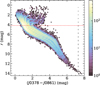 |
Fig. C.1 colour-magnitude diagram of the 4 × 4 mock catalog. |
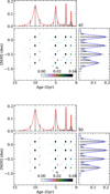 |
Fig. C.2 Input and recovered ages and metallicities for the 4 × 4 mock catalogue: (a) without and (b) with a prior distribution on [M/H]. The blue dashed lines represent the fit of a model composed of four normal distributions, while the red dashed lines show the fit using a combination of four Cauchy distributions. |
Appendix D Complementary results
Figure D.1 shows the distribution of [α/Fe] derived using GridE. These isochrones have only two α compositions; therefore, the mean [α/Fe] within each 0.2 × 0.2kpc2 pixel is determined by the relative number of stars with [α/Fe] = 0.0 or 0.4 dex. For this reason, a range of colours is visible in Fig. D.1. Low-α values (red pixels) are found closer to the Galactic plane and are concentrated towards the Galactic anticentre. This is consistent with the fact that the number of high-α stars, associated with the inner thick disc, drops significantly beyond the Sun’s position. High-α values (blue pixels) are found at larger vertical distances from the Galactic plane, consistent with the typical distribution of α-abundances in the Milky Way disc (Imig et al. 2023). Furthermore, high-α values dominate the pixel distribution for ages older than 10 Gyr.
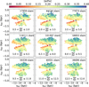 |
Fig. D.1 α-abundance map in galactocentric xGC and zGC coordinates of the JP×Gr16.55kpc (r ≤ 4.2 mag) sample. The [α/Fe]values were derived as described in Sec. 4.4, using Grid E. The colour-bar indicates the mean of [α/Fe]for stars within 0.2 × 0.2 kpc2 pixels. The pixels with less than 10 stars were rejected. |
We shows in this appendix the standard deviation the metal-licity age maps presented in Fig 9 and Fig 10.
All Tables
Isochrone Grids used in this work. The step in metallicity is ∆[M/H] = 0.1 dex for all the grids.
Standard deviation (σ) and FWHM of the Normal and Cauchy distributions, respectively, shown in Fig. C. The "No" and "yes" rows indicate the values obtained using and not-using a prior on [M/H], respectively. The bottom row shows the relative reduction on σ and FWHM.
All Figures
|
Fig. 1 Cumulative counts of JP×G , JP×G5kpc, and JP×G5kpc (J0378 < 0.1 mag) samples. The dash-dotted and dashed lines point out the limits r = 16.5 mag and r = 17.1 mag, where the JP×G5kpc and JP×G5kpc (J0378 < 0.1 mag) counts drop 10% below the JP×G counts. |
| In the text | |
|
Fig. 2 Hess diagram of JP×Gr16.55kpc sample for a) J0378 – J0861 and b) u – i. Panel c) shows the distribution of stars in the (r vs zGC) plane. The stellar colours and magnitudes are corrected by the effect of dust (Green et al. 2018; Schlafly & Finkbeiner 2011). The horizontal dotted line indicates the absolute r magnitude equal to 4.2 mag, separating the regions we used to extract the information of ages and metallicities. The arrow illustrates the dimming and reddening vector corresponding to AV = 1 mag. The crosses arranged vertically show the colour and magnitude average errors, computed for all star within interval of size ∆r = 1 mag. |
| In the text | |
|
Fig. 3 J-PLUS magnitude differences between solar-scaled and α-enhanced BaSTI models for MSTO stars. We selected three stellar pairs at [M/H] = −0.1 dex, with approximate ages of 2.5, 5.0, and 10 Gyr and corresponding masses of 1.3, 1.1, and 1.0 M⊙, respectively. The horizontal dashed line indicates the upper limit of the median absolutemagnitude error, as averaged from the third column of Table 1. |
| In the text | |
|
Fig. 4 Illustrative isochrone plot. Panel a displays a grid of nine isochrones with ages of 2.5, 5, and 10 Gyr and metallicities of [M/H] = −0.5, −0.2, and 0.1 dex. Isochrones with the same age are shown in green tones, illustrating the sensitivity of age and metallicity at the MSTO and the RGB phases. Panel b highlights the region of the CAMD where age sensitivity is highest (dashed polygon) using three isochrones of the same metallicity ([M/H] = −0.2 dex). The double-headed red arrow indicates the magnitude separation used to quantify the average distance between isochrones. Panel c shows the same grid as (a), but with orange tones indicating isochrones of the same metallicity. Panel d shows three isochrones of the same age (5 Gyr), illustrating how magnitude and colour vary with metallicity. The cyan arrow indicates the magnitude separation used to define the average distance between isochrones. |
| In the text | |
|
Fig. 5 Inferred metallicity distribution of JP×Gr16.55kpc sample (solid histogram) for stars with absolute r magnitudes fainter than 4.2 mag, using Grid A from Table 3. The dash-dotted line shows the metallicity distribution of an APOGEE DR17 sample, selected as described in Appendix A.2. The dashed line indicates the normal function adopted as the prior on [M/H] for the PARSEC models. |
| In the text | |
|
Fig. 6 Inferred SFH of JP×Gr16.55kpc sample for stars brighter than r = 4.2 mag, using Grid B. The grey histograms in the upper and right panels show the marginal distributions of age and metallicity, respectively. The red and blue error bars above the histograms indicate the full width at half maximum (FWHM) of the age and metallicity uncertainties, as estimated in Appendix C. The dashed and dash-dotted lines highlight the two population candidates that we consider to be detected. |
| In the text | |
|
Fig. 7 Inferred SFH of JP×Gr16.55kpc sample for stars brighter than r = 4.2 mag, using Grid C (solar-scaled; panel a) and Grid D (α-enhanced; panel b). The grey histograms in the upper and right panels show the marginal distributions of age and metallicity, respectively. The red and blue error bars above the histograms indicate the full width at half maximum (FWHM) of the age and metallicity uncertainties, as estimated in Appendix C. The dashed and dash-dotted lines highlight the two population candidates that we consider to be detected. |
| In the text | |
|
Fig. 8 Inferred SFH of JP×Gr16.55kpc sample for stars brighter than r = 4.2 mag, using Grid E, which simultaneously fits solar-scaled and α-enhanced isochrones (indicated as [a/Fe]=0.0 and [a/Fe]=0.4, respectively, in the panel titles). The grey histograms in the upper and right panels show the marginal distributions of age and metallicity, respectively. The red and blue error bars above the histograms represent the full width at half maximum (FWHM) of the age and metallicity uncertainties, as estimated in Appendix C. The dashed and dash-dotted lines highlight the two candidate populations that we consider to be detected. |
| In the text | |
|
Fig. 9 Metallicity map in galactocentric xGC and zGC coordinates of JP×Gr16.55kpc (r ≤ 4.2 mag) sample. The metallicity values were derived as described in Sect. 4.4, using Grid E (solar+α-enhanced isochrones) from Table 3. The colour bar indicates the mean of [M/H] for stars within 0.2 × 0.2 kpc2 pixels. The pixels with fewer than ten stars were rejected. |
| In the text | |
|
Fig. 10 Age map in galactocentric xGC and yGC coordinates of JP×Gr16.55kpc (r ≤ 4.2 mag) sample. The age values were derived as described in Sect. 4.4, using Grid E. The colour bar indicates the mean a for stars within 0.2 × 0.2 kpc pixels. The pixels with fewer than 10 stars were rejected. |
| In the text | |
|
Fig. C.1 colour-magnitude diagram of the 4 × 4 mock catalog. |
| In the text | |
|
Fig. C.2 Input and recovered ages and metallicities for the 4 × 4 mock catalogue: (a) without and (b) with a prior distribution on [M/H]. The blue dashed lines represent the fit of a model composed of four normal distributions, while the red dashed lines show the fit using a combination of four Cauchy distributions. |
| In the text | |
|
Fig. D.1 α-abundance map in galactocentric xGC and zGC coordinates of the JP×Gr16.55kpc (r ≤ 4.2 mag) sample. The [α/Fe]values were derived as described in Sec. 4.4, using Grid E. The colour-bar indicates the mean of [α/Fe]for stars within 0.2 × 0.2 kpc2 pixels. The pixels with less than 10 stars were rejected. |
| In the text | |
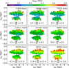 |
Fig. D.2 Standard deviation corresponding to the metallicity map in Fig 9. |
| In the text | |
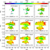 |
Fig. D.3 Standard deviation corresponding to the age map in Fig 10. |
| In the text | |
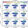 |
Fig. D.4 Standard deviation corresponding to the [α/Fe] map in Fig D.1. |
| In the text | |
Current usage metrics show cumulative count of Article Views (full-text article views including HTML views, PDF and ePub downloads, according to the available data) and Abstracts Views on Vision4Press platform.
Data correspond to usage on the plateform after 2015. The current usage metrics is available 48-96 hours after online publication and is updated daily on week days.
Initial download of the metrics may take a while.