| Issue |
A&A
Volume 706, February 2026
|
|
|---|---|---|
| Article Number | A360 | |
| Number of page(s) | 10 | |
| Section | The Sun and the Heliosphere | |
| DOI | https://doi.org/10.1051/0004-6361/202557119 | |
| Published online | 20 February 2026 | |
CLEAN and multiscale CLEAN for STIX in Solar Orbiter
1
MIDA, Dipartimento di Matematica, Università di Genova via Dodecaneso 35 16146 Genova, Italy
2
University of Applied Sciences and Arts Northwest Switzerland (FHNW), School of Computer Science Bahnhofstrasse 6 Windisch 5210, Switzerland
3
Osservatorio Astrofisico di Torino, Istituto Nazionale di Astrofisica via Osservatorio 20 10025 Pino Torinese, Italy
★ Corresponding authors: This email address is being protected from spambots. You need JavaScript enabled to view it.
; This email address is being protected from spambots. You need JavaScript enabled to view it.
; This email address is being protected from spambots. You need JavaScript enabled to view it.
Received:
5
September
2025
Accepted:
4
January
2026
Abstract
CLEAN is a well-established deconvolution approach to Fourier imaging at radio wavelengths and hard X-ray energies. One of the main limitations of CLEAN for hard X-ray imaging is that it requires a final convolution step by means of a convolution kernel whose width is strongly user dependent, and moreover, under-resolution effects are often introduced. This paper describes a multiscale version of CLEAN that is specifically tailored to the reconstruction of images from measurements observed by the Spectrometer/Telescope for Imaging X-rays (STIX) on board Solar Orbiter. Using synthetic STIX data, this study shows that multiscale CLEAN might represent a reliable solution to the two CLEAN limitations described above. Further, we show the performances of CLEAN and its multiscale release in reconstructing experimental real scenarios characterized by complex emission morphologies.
Key words: techniques: image processing / telescopes / Sun: flares / Sun: X-rays / gamma rays
© The Authors 2026
 Open Access article, published by EDP Sciences, under the terms of the Creative Commons Attribution License (https://creativecommons.org/licenses/by/4.0), which permits unrestricted use, distribution, and reproduction in any medium, provided the original work is properly cited.
This article is published in open access under the Subscribe to Open model. This email address is being protected from spambots. You need JavaScript enabled to view it. to support open access publication.
1. Introduction
The imaging concept for the most recent space missions in solar hard X-ray imaging is a Fourier transform model: Native measurements are samples of the Fourier transform of the incoming photon radiation, called visibilities, and image reconstruction in this framework therefore consists of solving the Fourier transform inversion problem from limited data (Bertero 2006). Previous examples of instruments that relied on this imaging approach are the Hard X-ray Space Telescope (HST) on board YohKoh (Kosugi et al. 1992), which used 32 pairs of modulation collimators to measure 32 visibilities in four broad bands in the energy range between 14 and 100 keV; and the Reuven Ramaty High Energy Solar Spectroscopic Imager (RHESSI; Lin et al. 2004), which observed hard X-rays and gamma-rays by means of nine rotating modulation collimators generating hundreds of visibilities with a heterogeneous signal-to-noise ratio. Two more Fourier-based space telescopes are currently flying to record hard X-ray observations of the Sun. Both of them are characterized by a Fourier-based technology. Specifically, on the one hand, the Spectrometer/Telescope for Imaging X-rays (STIX) on board Solar Orbiter (Benz et al. 2012; Krucker et al. 2020) works by using Moiré patterns and measures 30 visibilities from a complicated orbit that reaches distances to the Sun closer than Mercury. On the other hand, the Hard X-ray Imager (HXI) on board the Advanced Space-Based Solar Observatory (ASO-S) (Zhang et al. 2019) uses two subcollimators to measure the real and imaginary parts of 45 visibilities from an Earth orbit.
Within the framework of the RHESSI mission, several imaging methods have been developed, all designed to extract spatial information from the measured counts or visibilities (Hurford et al. 2002; Dennis & Pernak 2009; Schmahl et al. 2007; Benvenuto et al. 2013; Bong et al. 2006; Massa et al. 2020; Massone et al. 2009; Felix et al. 2017; Duval-Poo et al. 2018; Hannah et al. 2008; Aschwanden et al. 2002; Metcalf et al. 1996). In particular, image deconvolution based on CLEAN (Högbom 1974; Hurford et al. 2002) was the imaging tool applied for more than 10% of the RHESSI studies, which made this technique the most popular one in the RHESSI community. The steps of this algorithm consist of a CLEAN loop that generates a set of CLEAN components that are located where most of the source emission propagates; an estimate of the background; the sum of the CLEAN component map with the estimated background; and finally, the generation of the CLEANed map via convolution with an idealized point spread function (PSF) called the CLEAN beam.
It is well-established, however, that the CLEAN algorithm developed for RHESSI was affected by two main weaknesses: First, the degree of automation of CLEAN was rather limited, and the final convolution step was significantly dependent on the user choice. Second, the maps reconstructed by CLEAN are typically under-resolved, with a rather poor ability to identify different spatial scales in the field of view under analysis.
On the one hand, the first limitation has been addressed in Perracchione et al. (2023), who introduced an unbiased user-independent version of CLEAN for STIX. On the other hand, the formalism of a possible multiscale release of CLEAN has been outlined in Volpara et al. (2024) for the solution of the general Fourier transform inversion problem from limited data. These authors also briefly illustrated an application to RHESSI observations.
Our objective is to introduce the CLEAN and multiscale CLEAN algorithms into the STIX framework and to validate their performances against synthetic data and experimental observations. In particular, the multiscale version of the method relies on modeling the global PSF of the instrument as the sum of components, each of which corresponds to a specific collimator, so that grouping different collimators corresponds to obtaining different resolution powers. On the one hand, we proved in the simulated cases that when the user appropriately realizes this grouping, the corresponding reconstructions reproduce the different scales in the image well. On the other hand, we considered in the application to experimental data the flaring events on February, 24 2024, March, 10 2024, and May 14 2024, and compared the reconstructions provided by CLEAN and multiscale CLEAN for the STIX data with images of the same events provided by the Atmospheric Imaging Assembly (AIA) on board the Solar Dynamics Observatory (SDO) in the extreme-ultraviolet (EUV) regime (Lemen et al. 2012) and by the HXI on board ASO-S, again in the case of hard X-ray energies (Zhang et al. 2019).
The plan of the paper is as follows. Section 2 illustrates the possible design of CLEAN and multiscale CLEAN for processing STIX data. Section 3 validates the multiscale approach in the case of synthetic visibilities. Section 4 applies multiscale CLEAN to the analysis of STIX measurements recorded during three flaring events in 2024. Our conclusions are offered in Sect. 5.
2. CLEAN in the STIX framework
The deconvolution algorithm CLEAN was introduced by Högbom (1974) for radioastronomy imaging and was translated into a solar hard X-ray context (Hurford et al. 2002) for the processing of data recorded by the Reuven Ramaty High Energy Solar Spectroscopic Imager (RHESSI). The basic idea behind CLEAN is that the image to be reconstructed can be represented as the superposition of point sources that are iteratively introduced in the reconstruction process. More schematically, CLEAN is implemented by means of the following steps:
-
A dirty map of the hard X-ray emission is obtained by applying the discrete Fourier transform to the set of visibilities recorded during a specific time interval and in correspondence with a specific photon energy channel.
-
After identifying the maximum in the dirty map, a CLEAN component map is generated by means of a δ-Dirac placed at the maximum position.
-
The dirty beam, that is, the instrument PSF, centered at the maximum position, is then subtracted from the dirty map.
Items 2 and 3 are iterated until the remaining dirty map contains just noise, and the final CLEANed image is obtained by adding an estimate of the residuals to the CLEAN component map and then convolving with the so-called CLEAN beam, that is, an idealized form of the instrument PSF obtained by fitting the dirty beam by means of an idealized two-dimensional Gaussian function.
As shown in Fig. 1, this scheme depends on the properties of the telescope at different levels, which affects its implementation within the STIX framework. First, the sampling of the spatial frequency plane (the (u, v) plane hereafter) is significantly different; this implies different properties of the instrumental PSFs and, specifically, of the shapes of their central peaks, which are a measure of the spatial resolution achievable by the two instruments. As a consequence, this difference in the resolution power is reflected by the different full width at half maximum (FWHM) of the RHESSI and STIX CLEAN beam. Specifically, on the one hand, the nominal maximum RHESSI angular resolution was 2.26 arcsec. On the other hand, STIX achieves a nominal maximum resolution of 7.2 arcsec, although at the current stage of the calibration process, collimators 1 and 2 are not included in the imaging process, so that the maximum resolution decreases to 14.6 arcsec. Solar Orbiter can approach the Sun as close as 0.28 astronomical units (AU), however. At this distance, an angular resolution of 1 arcsecond corresponds to a linear scale of about 200 km on the solar surface, compared to roughly 725 km per arcsecond at 1 AU (the Earth–Sun distance, relevant for RHESSI). Although the nominal angular resolution of STIX is lower than that of RHESSI, the much closer observing distance effectively compensates for this limitation in this way and provides a comparable or even superior spatial resolving power on the Sun.
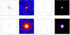 |
Fig. 1. Comparison between the imaging characteristics of RHESSI (top row) and STIX (bottom row). First column: Sampling of the (u, v) plane. Second column: PSFs. Third column: Central cut of the PSFs. Fourth column: Idealized PSFs obtained by fitting the central peak of the original PSFs. The top left panel describes a typical experimental (u, v) sampling from which some of the sampling points are missing because the corresponding visibilities did not pass the statistical quality check test. |
The experience of using CLEAN for the analysis of RHESSI visibilities showed that this imaging approach has two main limitations. First, CLEAN is not capable of automatically adapting to the spatial scale of the source to be reconstructed, which often results in under-resolution effects in reconstructions. Second, the step implementing the convolution between the CLEAN component map and the CLEAN beam is significantly user dependent because the FHWM of the CLEAN beam is typically tuned according to heuristic considerations. Very recently, Volpara et al. (2024) formulated a multiscale version of CLEAN that does not require the final convolution step and that was validated against synthetic and experimental RHESSI data. For RHESSI, this multiscale CLEAN method for STIX also explicitly leverages the fact that the sampling of the Fourier transform is made over disjoint circles in the (u, v) plane, so that the corresponding PSF can be rearranged into contributions that each refer to a specific circle.
Specifically, the starting points for multiscale CLEAN in the case of STIX visibilities are, first, to group the set of ten circles characterizing the STIX (u, v) plane into N subsets and to model the image I(x, y) to reconstruct according to the formula
 (1)
(1)
which assumes that for each subset, an unknown image exists that can be modeled as the sum of Qi normalized basis functions mi(x, y), each centered at (xqi, yqi) and with a peak intensity Iqi. Second, for each subset, the corresponding dirty map is computed by applying the inverse Fourier transform to the Fourier samples corresponding to each subset. Third, the corresponding PSF is computed for each subset. Denoting a map made of pixels with zero content by CC(0)(x, y), the first iteration is computed according to a process that reads as follows:
-
Each dirty map Ij(0), j = 1, …, N, is rescaled according to the rule described in Volpara et al. (2024), that is, each map is pixel-wise divided by its maximum and multiplied by a bias factor that decreases as j increases in order to favor small scales at the first iterations.
-
The first selected scale is identified among all dirty maps as the scale corresponding to the rescaled dirty map with the maximum intensity value (rescaled dirty maps are used in this step alone, i.e., for maximum identification). Then, the corresponding PSF K(x, y) and the corresponding basis function m(x, y) are selected.
-
The multiscale CLEAN components map is computed as
 (2)
(2)where Imax is the maximum value of the dirty map at the selected scale, (xmax, ymax) denotes its position, and γ is a gain factor.
-
At each scale j = 1, …, N, the dirty map component is computed in such a way that
 (3)
(3)
Iterations continue while CC(x, y) is accordingly updated, until a stopping rule is satisfied.
In the final step of multiscale CLEAN, no convolution with any CLEAN beam is needed, and the CLEANed map C(x, y) is constructed as
 (4)
(4)
where CC(L)(x, y) is given by (2) at the last iteration, and B′(x, y) is an estimate of the background.
3. Validation with synthetic STIX visibilities
The standard model for solar flares (Tandberg-Hanssen & Emslie 1988; Piana et al. 2022) implies that the emitting configurations may involve a coronal loop corresponding to thermal energies that is characterized by an elliptic shape in several cases; and by two circular sources at higher nonthermal energies (depending on the position of the footpoints with respect to the limb, only one source may be visible to the telescope). Accounting for this scenario, we generated synthetic sets of STIX visibilities corresponding to five different configurations:
-
A single circular Gaussian source.
-
A single Gaussian elliptic source.
-
A single loop, obtained by bending the elliptic source.
-
Two approaching circular Gaussian footpoints.
-
Two circular Gaussian sources with significantly different size.
-
A configuration made of one large loop and a small circular Gaussian source.
In order to quantitatively assess the performances of CLEAN and multiscale CLEAN, we considered the capability of the algorithms to reconstruct the following imaging parameters:
-
The total flux of the emitting source.
-
The position of the flux peak.
-
The values of the FWHM along both axes.
-
The maximum intensity of each source.
After giving specific values to these parameters, we generated the ground truth maps using the same code as applied by Volpara et al. (2022) to generate the ground truth maps used to validate the particle swarm optimization algorithm, and providing each map with 10 000 counts s−1 cm−2 keV−1. Then, we computed the corresponding STIX synthetic visibility sets by computing the Fourier transform of these images sampled in correspondence of the (u, v) points characterizing the STIX design. Specifically, we assumed that only collimators from 3 through 10 were available because the calibration process concerned with the highest resolution collimators is not yet finalized.
Figure 2 and Table 1 qualitatively and quantitatively compare the reconstructions provided by CLEAN and multiscale CLEAN with the ground truth and with the reconstructions obtained by means of constrained maximum entropy (Massa et al. 2020), an interpolation/extrapolation algorithm (Perracchione et al. 2021), and an unbiased version of CLEAN based on feature augmentation (Perracchione et al. 2023) for the three single-source configurations. We chose a two-scale setup for multiscale CLEAN. Specifically, for the circular Gaussian and loop-like sources, the two scales were realized by grouping detectors 3 through 9 for the high-resolution scale and using detector 10 for the low-resolution scale; for the elliptical source, the two scales were obtained by grouping detectors 3 through 7 and detectors 8 through 10, respectively. These results show that CLEAN and its multiscale version are able to model the correct shape of the flaring sources, although multiscale CLEAN performs better than standard CLEAN in the estimate of the total and maximum fluxes; further, its performances are comparable with those provided by the other three methods for the circular source, but they are more accurate for the ellipse and the loop. Interestingly, the results of multiscale CLEAN were obtained by setting the algorithm in a two-scale configuration, which shows its flexibility in adapting the setting performances to the input data.
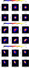 |
Fig. 2. Reconstruction of a single source. Comparison between the ground truth and the performances provided CLEAN, multiscale CLEAN, constrained maximum entropy (MEM_GE), an interpolation/extrapolation algorithm (uv_smooth_VSK), and a version of CLEAN based on feature augmentation (u_CLEAN). First two rows: Circular Gaussian source. Second two rows: Loop-shaped source. Third two rows: Elliptical source. The corresponding imaging parameters are listed in Table 1. |
We then considered three two-source configurations, in which two Gaussian sources with equal total flux gradually brought approached each other. The total flux for the reconstruction was again 104 counts s−1 cm−2 keV−1, and multiscale CLEAN was applied in a two-scale setup (detectors 3 through 7 for the first scale, and detectors 8 through 10 for the second scale). The results in Fig. 3 and Table 2 show that CLEAN and multiscale CLEAN were able to reconstruct the morphology of the two-source configurations, although the multiscale algorithm preserves the circular shapes better. Further, the parametric performances of multiscale CLEAN are significantly more robust than those associated with the other algorithms while the two sources approach each other, with this algorithm being more effective in reproducing the total flux and local maxima. In particular, the values of the FWHM provided by multiscale CLEAN recover those better that are associated with the ground truth, showing that the multiscale release improves the under-resolution issue characterizing standard CLEAN performances. Further, multiscale CLEAN reduces the artifacts in the region between the two peaks.
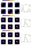 |
Fig. 3. Reconstruction of two approaching circular Gaussian sources. Comparison between the ground truth (first column) and the performances of CLEAN, multiscale CLEAN, and the other algorithms considered in Fig. 2. The fourth column compares the profiles along the cut across the source peaks. |
The final analysis in the synthetic setting was concerned with two sources with significantly different sizes and the same peak intensity, which is probably the most indicative test for validating the effectiveness of a multiscale approach. For reconstructing the configuration with two circular sources, multiscale CLEAN was applied using three scales that were obtained by grouping detectors 3 and 4 (first scale), detectors 5 through 8 (second scale), and detectors 9 and 10 (third scale). To reconstruct the configuration made of the large loop and the small circular source, we used two scales made of detectors 3 through 8 and detectors 9 and 10. Table 3 shows the input and reconstructed parameters corresponding to the reconstructions in Fig. 4. The multiscale approach again outperforms standard CLEAN in estimating the imaging parameters, although it has some difficulties in accurately reproducing the exact loop shape. In this case, multiscale CLEAN also performs very well for the photometry and for the determination of most of the geometrical parameters.
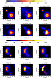 |
Fig. 4. Reconstruction of two sources with different sizes. Comparison between the ground truth and the reconstructions provided by CLEAN, multiscale CLEAN, and the other algorithms considered in Figs. 2 and 3. In the first two rows, both sources are modeled by a circular Gaussian function, and in the second two rows, the largest source has a loop shape. |
4. Analysis of real flaring events
The application of CLEAN and multiscale CLEAN to visibilities recorded by STIX is concerned with three events occurred on February, 24 2024, March, 10 2024, and May, 14 2024. All three events were observed from Earth orbits and the Solar Orbiter. We therefore generated for each event the EUV map from data recorded by SDO/AIA at 1600 Å (for the February 24-2024 and March 10-2024 flares) and at 131 Å (for the May 14-2024 flare). Further, since in the case of real events no ground truth is at our disposal, we considered measurements of the flaring radiation collected by the HXI on board the Chinese cluster ASO-S, which leverages an imaging modality very similar to the one used by the ESA telescope.
The results of this analysis are shown in Fig. 5, which allows us to qualitatively assess the CLEAN and multiscale CLEAN performances to interpretat the experimental visibilities of STIX. For each data set, we superimposed the level curves corresponding to the CLEAN and multiscale CLEAN reconstructions onto the AIA EUV maps that were appropriately reprojected in order to account for the different relative positions of the two instruments with respect to the flaring source. The same procedure was followed by using the level curves provided by
-
A constrained maximum entropy method implemented in the MEM_GE routine (Massa et al. 2020), which is often considered as the imaging benchmark by the STIX community, and
-
A CLEAN algorithm applied on a dataset recorded by HXI in (approximately) the same time range and for the same energy channel.
The CLEAN method we used to analyze the HXI observations used counts as input because the calibration process of the visibilities for the Chinese instrument is not yet finalized. The purpose of the tests in Fig. 5 was to first of all assess the performance of multiscale CLEAN qualitatively while comparing the morphologies of the reconstructions from STIX data with those provided by a very standard algorithm applied to HXI data. This comparison is particularly tight in the first two cases, and less so in the third case, where the viewpoints of the two telescopes differ significantly. Nevertheless, even in this third case, the reconstruction provided by multiscale CLEAN appears to confirm its reliability qualitatively.
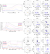 |
Fig. 5. Multiscale CLEAN for three real events observed by STIX: the February 24 2024 event in the time range 06:27:00–06:29:00 UT and for the 25–50 keV energy channel (first row); the March 10 2024 event in the time range 12:05:00–12:07:00 UT and for the 22–50 keV energy channel (second row); and the May 14 2024 event in the time range 12:46:55–12:47:55 UT for the 32–76 keV (third row). The first column contains the light curves. The second column provides the AIA map at 1600 Å for February 24 and March 10, at 131 Å for May 14 (top left panel); the HXI level curves reconstructed by CLEAN (top middle panel); the STIX level curves reconstructed by MEM_GE (top right panel); the position of the Earth and of Solar Orbiter at the event (bottom left panel); the STIX level curves reconstructed by CLEAN (bottom middle panel); and the STIX level curves reconstructed by multiscale CLEAN (bottom right panel). All level curves are superimposed onto the AIA map. The HXI observations are made in the 06:31:02–06:31:42 UT time interval and for the 25–50 keV energy channel for the first event; in the 12:10:00–12:11:00 UT time interval and for the 22–50 keV energy channel for the second event; andin the 12:46:45–12:47:00 UT time interval and for the 35–55 keV energy channel for the third event. |
The different imaging approaches are compared in Table 4 by computing the χ2 values1 predicted by the CLEAN component map and the CLEAN, multiscale CLEAN and MEM_GE reconstructions for the STIX visibilities. We did not compute any statistical metric for HXI because the count uncertainties are not yet available for this instrument, and the visibility uncertainties were approximated as 10% of the maximum observed visibility amplitude. Because these error estimates are not derived from the actual noise properties of the data, the resulting metrics ( χ2 and C-statistic) cannot be interpreted as statistically meaningful confidence levels.
5. Conclusions
We introduced a computational tool for image reconstruction from STIX observations that is based on a multiscale version of CLEAN and compared its performances with those provided by a standard CLEAN deconvolution. The analysis of synthetic visibilities showed that multiscale CLEAN outperforms standard CLEAN in the ability to qualitatively reproduce the ground truth shape even for single-scale flaring sources. From a more quantitative point of view, however, the parameters that describe the different properties of the source are reconstructed with a similar precision from the perspective of the first three moments (flux, position, and size). The reconstructions provided by multiscale CLEAN for experimental measurements are clearly better resolved than those provided by CLEAN and are rather similar to those corresponding to the use of MEM_GE. This trend is quantitatively confirmed by the values of the corresponding goodness of fit measured by χ2 (for CLEAN, multiscale CLEAN, and MEM_GE applied to STIX visibilities). The next step for the development of the multiscale approach for STIX visibilities will be the integration of the tool2 with an algorithm that can automatically choose the number of scales based on the input data.
Acknowledgments
Solar Orbiter is a space mission of international collaboration between ESA and NASA, operated by ESA. The STIX instrument is an international collaboration between Switzerland, Poland, France, Czech Republic, Germany, Austria, Ireland, and Italy. AV, MP, and AMM are supported by the ‘Accordo ASI/INAF Solar Orbiter: Supporto scientifico per la realizzazione degli strumenti Metis, SWA/DPU e STIX nelle Fasi D-E’. MP acknowledges the support of the PRIN PNRR 2022 Project ‘Inverse Problems in the Imaging Sciences (IPIS)’ 2022ANC8HL, cup: D53D23005740006. The research by AV, AMM, and MP was performed within the framework of the MIUR Excellence Department Project awarded to Dipartimento di Matematica, Università di Genova, CUP D33C23001110001. PM acknowledges support from the Swiss National Science Foundation in the framework of the project Robust Density Models for High Energy Physics and Solar Physics (rodem.ch), CRSII5_193716. AV, AMM, and MP also acknowledge the support of the Fondazione Compagnia di San Paolo within the framework of the Artificial Intelligence Call for Proposals, AIxtreme project (IDRol: 71708). AV also aknowledges the GNCS-INdAM PIANIS project “Problemi Inversi e Approssimazione Numerica in Imaging Solare”.
References
- Aschwanden, M. J., Schmahl, E., & Team, T. R. 2002, Sol. Phys., 210, 193 [NASA ADS] [CrossRef] [Google Scholar]
- Benvenuto, F., Schwartz, R., Piana, M., & Massone, A. M. 2013, A&A, 555, A61 [NASA ADS] [CrossRef] [EDP Sciences] [Google Scholar]
- Benz, A. O., Krucker, S., Hurford, G. J., et al. 2012, in Space Telescopes and Instrumentation 2012: Ultraviolet to Gamma Ray, eds. T. Takahashi, S. S. Murray, & J. W. A. den Herder, SPIE Conf. Ser., 8443, 84433L [Google Scholar]
- Bertero, M. 2006, Inverse Problems: Lectures given at the 1st1986 Session of the Centro Internazionale Matematico Estivo (CIME) held at Montecatini Terme, Italy, May 28-June 5, 1986 (Springer) [Google Scholar]
- Bong, S.-C., Lee, J., Gary, D. E., & Yun, H. S. 2006, ApJ, 636, 1159 [Google Scholar]
- Dennis, B. R., & Pernak, R. L. 2009, ApJ, 698, 2131 [NASA ADS] [CrossRef] [Google Scholar]
- Duval-Poo, M. A., Piana, M., & Massone, A. M. 2018, A&A, 615, A59 [NASA ADS] [CrossRef] [EDP Sciences] [Google Scholar]
- Felix, S., Bolzern, R., & Battaglia, M. 2017, ApJ, 849, 10 [NASA ADS] [CrossRef] [Google Scholar]
- Hannah, I. G., Christe, S., Krucker, S., et al. 2008, ApJ, 677, 704 [NASA ADS] [CrossRef] [Google Scholar]
- Högbom, J. A. 1974, A&AS, 15, 417 [Google Scholar]
- Hurford, G. J., Schmahl, E. J., Schwartz, R. A., et al. 2002, Sol. Phys., 210, 61 [Google Scholar]
- Kosugi, T., Sakao, T., Masuda, S., et al. 1992, PASJ, 44, L45 [NASA ADS] [Google Scholar]
- Krucker, S., Hurford, G. J., Grimm, O., et al. 2020, A&A, 642, A15 [NASA ADS] [CrossRef] [EDP Sciences] [Google Scholar]
- Lemen, J. R., Title, A. M., Akin, D. J., et al. 2012, Sol. Phys., 275, 17 [Google Scholar]
- Lin, R. P., Dennis, B., Hurford, G., Smith, D. M., & Zehnder, A. 2004, in Telescopes and Instrumentation for Solar Astrophysics, eds. S. Fineschi, & M. A. Gummin, SPIE Conf. Ser., 5171, 38 [Google Scholar]
- Massa, P., Schwartz, R., Tolbert, A. K., et al. 2020, ApJ, 894, 46 [NASA ADS] [CrossRef] [Google Scholar]
- Massone, A. M., Emslie, A. G., Hurford, G. J., et al. 2009, ApJ, 703, 2004 [NASA ADS] [CrossRef] [Google Scholar]
- Metcalf, T. R., Hudson, H. S., Kosugi, T., Puetter, R. C., & Pina, R. K. 1996, ApJ, 466, 585 [CrossRef] [Google Scholar]
- Perracchione, E., Massa, P., Massone, A. M., & Piana, M. 2021, ApJ, 919, 133 [NASA ADS] [CrossRef] [Google Scholar]
- Perracchione, E., Camattari, F., Volpara, A., et al. 2023, ApJS, 268, 68 [NASA ADS] [CrossRef] [Google Scholar]
- Piana, M., Emslie, A. G., Massone, A. M., & Dennis, B. R. 2022, Hard X-ray Imaging of Solar Flares (Springer), 164 [Google Scholar]
- Schmahl, E. J., Pernak, R. L., Hurford, G. J., Lee, J., & Bong, S. 2007, Sol. Phys., 240, 241 [Google Scholar]
- Tandberg-Hanssen, E., & Emslie, A. G. 1988, The Physics of Solar Flares (Cambridge: University Press) [Google Scholar]
- Volpara, A., Massa, P., Perracchione, E., et al. 2022, A&A, 668, A145 [NASA ADS] [CrossRef] [EDP Sciences] [Google Scholar]
- Volpara, A., Catalano, M., Piana, M., & Maria Massone, A. 2024, Inverse Problems, 40, 125017 [Google Scholar]
- Zhang, Z., Chen, D.-Y., Wu, J., et al. 2019, Res. Astron. Astrophys., 19, 160 [CrossRef] [Google Scholar]
The χ2 values are computed using the same formula as in Eq. (4) of Volpara et al. (2022) with Nθ = 1.
Multi-scale CLEAN codes are available at the MIDA group GitHub https://github.com/theMIDAgroup/MultiScaleCLEAN_codes
All Tables
All Figures
|
Fig. 1. Comparison between the imaging characteristics of RHESSI (top row) and STIX (bottom row). First column: Sampling of the (u, v) plane. Second column: PSFs. Third column: Central cut of the PSFs. Fourth column: Idealized PSFs obtained by fitting the central peak of the original PSFs. The top left panel describes a typical experimental (u, v) sampling from which some of the sampling points are missing because the corresponding visibilities did not pass the statistical quality check test. |
| In the text | |
|
Fig. 2. Reconstruction of a single source. Comparison between the ground truth and the performances provided CLEAN, multiscale CLEAN, constrained maximum entropy (MEM_GE), an interpolation/extrapolation algorithm (uv_smooth_VSK), and a version of CLEAN based on feature augmentation (u_CLEAN). First two rows: Circular Gaussian source. Second two rows: Loop-shaped source. Third two rows: Elliptical source. The corresponding imaging parameters are listed in Table 1. |
| In the text | |
|
Fig. 3. Reconstruction of two approaching circular Gaussian sources. Comparison between the ground truth (first column) and the performances of CLEAN, multiscale CLEAN, and the other algorithms considered in Fig. 2. The fourth column compares the profiles along the cut across the source peaks. |
| In the text | |
|
Fig. 4. Reconstruction of two sources with different sizes. Comparison between the ground truth and the reconstructions provided by CLEAN, multiscale CLEAN, and the other algorithms considered in Figs. 2 and 3. In the first two rows, both sources are modeled by a circular Gaussian function, and in the second two rows, the largest source has a loop shape. |
| In the text | |
|
Fig. 5. Multiscale CLEAN for three real events observed by STIX: the February 24 2024 event in the time range 06:27:00–06:29:00 UT and for the 25–50 keV energy channel (first row); the March 10 2024 event in the time range 12:05:00–12:07:00 UT and for the 22–50 keV energy channel (second row); and the May 14 2024 event in the time range 12:46:55–12:47:55 UT for the 32–76 keV (third row). The first column contains the light curves. The second column provides the AIA map at 1600 Å for February 24 and March 10, at 131 Å for May 14 (top left panel); the HXI level curves reconstructed by CLEAN (top middle panel); the STIX level curves reconstructed by MEM_GE (top right panel); the position of the Earth and of Solar Orbiter at the event (bottom left panel); the STIX level curves reconstructed by CLEAN (bottom middle panel); and the STIX level curves reconstructed by multiscale CLEAN (bottom right panel). All level curves are superimposed onto the AIA map. The HXI observations are made in the 06:31:02–06:31:42 UT time interval and for the 25–50 keV energy channel for the first event; in the 12:10:00–12:11:00 UT time interval and for the 22–50 keV energy channel for the second event; andin the 12:46:45–12:47:00 UT time interval and for the 35–55 keV energy channel for the third event. |
| In the text | |
Current usage metrics show cumulative count of Article Views (full-text article views including HTML views, PDF and ePub downloads, according to the available data) and Abstracts Views on Vision4Press platform.
Data correspond to usage on the plateform after 2015. The current usage metrics is available 48-96 hours after online publication and is updated daily on week days.
Initial download of the metrics may take a while.