| Issue |
A&A
Volume 706, February 2026
|
|
|---|---|---|
| Article Number | A362 | |
| Number of page(s) | 11 | |
| Section | Cosmology (including clusters of galaxies) | |
| DOI | https://doi.org/10.1051/0004-6361/202557361 | |
| Published online | 20 February 2026 | |
Tracing the high-z cosmic web with Quaia: Catalogues of voids and clusters in the quasar distribution
1
Institute of Astronomy and NAO, Bulgarian Academy of Sciences 72 Tsarigradsko Chaussee Blvd. 1784 Sofia, Bulgaria
2
MTA–CSFK Lendület “Momentum” Large-Scale Structure (LSS) Research Group Konkoly Thege Miklós út 15-17 H-1121 Budapest, Hungary
3
Konkoly Observatory, HUN-REN Research Centre for Astronomy and Earth Sciences Konkoly Thege Miklós út 15-17 H-1121 Budapest, Hungary
4
Instituto de Astrofísica de Canarias Calle Via Láctea s/n E-38205 La Laguna Tenerife, Spain
5
Departamento de Astrofísica, Universidad de La Laguna E-38206 La Laguna Tenerife, Spain
6
Institute of Physics and Astronomy, ELTE Eötvös Loránd University Pázmány Péter sétány 1/A H-1117 Budapest, Hungary
7
Département d’Astronomie, Université de Genève Chemin Pegasi 51 CH-1290 Versoix, Switzerland
8
Institut für Astrophysik, Universität Zürich Winterthurerstrasse 190 CH-8057 Zürich, Switzerland
★ Corresponding author: This email address is being protected from spambots. You need JavaScript enabled to view it.
Received:
22
September
2025
Accepted:
22
November
2025
Abstract
Context. Understanding the formation and evolution of the cosmic web of galaxies is a fundamental goal of both theoretical and observational cosmology, which use various tracers of the cosmic large-scale structure at an ever wider range of redshifts.
Aims. Our principal aim is to advance the mapping of the cosmic web at high redshifts using observational and synthetic catalogues of quasars , which offer a powerful probe of structure formation and the validity of the concordance cosmological model at the largest scales in the Universe.
Methods. In this analysis, we selected 708 483 quasars at 0.8 < z < 2.2 from the Quaia dataset; this enabled an extended reconstruction of the matter density field using 24 372 deg2 sky area with a well-understood selection function, thus going beyond the capacity of previous studies. Using the REVOLVER method, we created catalogues of voids and clusters based on the estimation of the local density at quasar positions with Voronoi tessellation. We tested the consistency of Quaia data and 50 realistic mock catalogues, including various parameters of the voids and clusters in characteristic subsets of the data, and also measurements of the density profiles of these cosmic super-structures at R ≈ 100 h−1 Mpc scales.
Results. We identified 12 820 voids and 41 154 clusters in the distribution of Quaia quasars. We found an ∼5 − 10% level of agreement between data and the ensemble of the 50 mocks considering void and cluster radii, average inner density, and density profiles at all redshifts. In particular, we tested the role of survey mask proximity effects in void and cluster detection, which, although present in the data, are consistent in simulations and observations. Testing the extremes, the largest voids and clusters reach Reff ≈ 250 h−1 Mpc and Reff ≈ 150 h−1 Mpc, respectively, but without evidence for ultra-large cosmic structures exceeding the dimensions of the largest structures in our mock catalogues.
Conclusions. Our data-analysis results highlight the capacity of Quaia quasars to robustly map the high-z cosmic web, further supported by the fully consistent statistical results from 50 mock catalogues. As an important deliverable, we share our density field estimation, void catalogues, and cluster catalogues with the public, which allows various additional cross-correlation probes in the high-z cosmic web.
Key words: catalogs / surveys / large-scale structure of Universe
© The Authors 2026
 Open Access article, published by EDP Sciences, under the terms of the Creative Commons Attribution License (https://creativecommons.org/licenses/by/4.0), which permits unrestricted use, distribution, and reproduction in any medium, provided the original work is properly cited.
This article is published in open access under the Subscribe to Open model. This email address is being protected from spambots. You need JavaScript enabled to view it. to support open access publication.
1. Introduction
Mapping out the intricate cosmic web of galaxies is a major goal of observational cosmology that motivates deep and wide sky survey projects (see e.g. The Dark Energy Survey Collaboration 2005; Levi et al. 2013; Amendola et al. 2013; LSST Science Collaboration 2009) as well as various numerical simulation approaches (see e.g. Cai et al. 2009; Potter et al. 2016; Takahashi et al. 2017; Rácz et al. 2023; Schaye et al. 2023). The largest and in many senses most extreme objects in this cosmic large-scale structure (LSS) are the superclusters of galaxies and the cosmic voids, where the density of galaxies is significantly lower than the average. These superstructures appear at 10−100 megaparsec scales and offer insights into gravitational evolution, galaxy formation, and the underlying cosmological model (see e.g. Pisani et al. 2019). Moreover, their spatial distribution and statistical properties also provide a unique opportunity to test the cosmological principle – the assumption that the Universe is statistically homogeneous and isotropic on the largest scales.
In particular, cosmic voids have received increasing attention in recent years as cosmological probes due to their sensitivity to dark energy, modified gravity, neutrino mass, and primordial non-Gaussianity, among other phenomena (see e.g. Clampitt et al. 2013; Cai et al. 2015; Kitaura et al. 2016; Cautun et al. 2018; Baker et al. 2018; Schuster et al. 2019; Davies et al. 2021; Contarini et al. 2021; Vielzeuf et al. 2023). Voids constrain cosmological models through various probes, such as the void size function, density and velocity profiles, lensing effects, and their evolution with redshift (see e.g. Amendola et al. 1999; Krause et al. 2013; Pisani et al. 2015; Sánchez et al. 2017; Fang et al. 2019; Nadathur et al. 2019; Hamaus et al. 2021).
Another active area of research has been to cross-correlate the positions of cosmic voids with the cosmic microwave background (CMB). Their imprints in CMB lensing convergence maps (see e.g. Cai et al. 2013; Raghunathan et al. 2020; Kovács et al. 2022a; Camacho-Ciurana et al. 2024; Sartori et al. 2025), in Compton y-maps to study the thermal Sunyaev-Zeldovich (tSZ) effect (Alonso et al. 2018; Li et al. 2024), and in temperature maps via the integrated Sachs-Wolfe (ISW) effect (see e.g. Sachs & Wolfe 1967) have all been measured extensively, often with intriguing tensions (see e.g. Granett et al. 2008; Ilić et al. 2013; Kovács et al. 2017; Nadathur & Crittenden 2016; Kovács et al. 2019).
While low-redshift galaxy surveys such as Sloan Digital Sky Survey (SDSS), Baryon Oscillation Spectroscopic Survey (BOSS), Dark Energy Survey (DES), and more recently Dark Energy Spectroscopic Instrument (DESI) survey have enabled detailed reconstructions of the galaxy density field and the creation of void catalogues up to z ∼ 0.8 (see e.g. Mao et al. 2017; Douglass et al. 2023; Rincon et al. 2025), the intermediate redshift regime 0.8 < z < 2.2 in the cosmic web, which is studied in this analysis, remains relatively uncharted. In this range, currently available galaxy samples are sparse and quasars provide the best available tracers of the underlying dark matter distribution, due to their brightness. The extended Baryon Oscillation Spectroscopic Survey (eBOSS) facilitated one of the first statistical void analyses at these redshifts using spectroscopic quasars, including the 3D void catalogues by Hawken et al. (2017) and Aubert et al. (2022), and 2D void catalogues by Kovács et al. (2022b). While providing a rather small sky coverage for accurate statistics (approx. 4800 deg2 in Data Release 16), these analyses demonstrated the viability of using quasars to probe the cosmic large-scale structure at high redshift, despite their low spatial density.
Recent years have also witnessed growing interest in identifying large-scale overdensities, such as superclusters and quasar groups (see e.g. Park et al. 2015; Einasto et al. 2021; Liu et al. 2024). Superclusters, the most massive coherent structures in the cosmic web, provide critical insights into the non-linear regime of structure formation and the transition between filamentary and cluster-dominated environments. A number of studies have analysed galaxy and quasar surveys to detect such structures, using methods ranging from friends-of-friends linking algorithms to percolation analysis and minimal spanning trees (see e.g. Libeskind et al. 2018; Naidoo et al. 2020). In particular, among several ultra-large structures (see e.g. Lopez et al. 2022; Horvath et al. 2025), large quasar groups (LQGs) have been reported at higher redshifts, extending over several hundred comoving megaparsecs (such as the Huge-LQG, see Clowes et al. 2014). While the statistical significance and cosmological implications of these LQGs remain debated, they have raised questions about the validity of the cosmological principle (see e.g. Nadathur 2013; Sawala et al. 2025) and their detection motivates the use of increasingly large and homogeneous quasar samples for cosmic web analysis.
To advance this line of research, we used the recent Quaia quasar catalogue (Storey-Fisher et al. 2024) that provides an all-sky sample of quasars with precise photometric redshifts (see e.g. Piccirilli et al. 2024; Veronesi et al. 2025; Fabbian et al. 2025; Alonso et al. 2025, for previous applications). We mapped the cosmic large-scale structure at 0.8 < z < 2.2 using this catalogue and focused on the identification of the largest voids and (super)clusters traced by the quasar distribution. Since the exact properties of such extreme structures may challenge our understanding of cosmic variance and structure formation in the standard Λ cold dark matter (ΛCDM) model, a more inclusive census of these cosmic superstructures at high redshift from the Quaia dataset might help resolve any related tension. We note that extensions of the Quaia cosmic web analyses to higher redshifts are also feasible, especially using the next Gaia data release (DR4) to possibly increase the quasar source density.
Our analysis results in two main products. First, we estimate the local overdensity at the position of each quasar. Second, we provide a catalogue of voids and clusters identified in the Quaia quasar distribution. The combination of these enables future studies to examine quasar properties, such as luminosity or spectral features, as a function of their cosmic environment.
The paper is organized as follows. In Section 2, we introduce our observational and mock datasets, as well as our methodology. Section 3 contains a description of our analysis of the reconstructed density field of the quasars, including catalogues of voids and clusters, followed by a summary of our main conclusions in Section 4.
2. Datasets and methodology
2.1. Quasar catalogue
In our cosmographical analysis, we used the Quaia quasar catalogue (Storey-Fisher et al. 2024), based on a cross-match between the Gaia Data Release 3 quasar candidates (Gaia Collaboration 2023a,b; Delchambre et al. 2023) and the Wide-field Infrared Survey Explorer (WISE, Lang 2014) dataset. This cleaned catalogue exploits segmentation in colour-colour spaces to differentiate stars, galaxies, and quasars, and excludes sources with high proper motions. The Quaia catalogue comes in two versions; the full dataset contains approximately 1.3 million quasars with G < 20.5 (this is what we work with), while a higher fidelity G < 20.0 subsample is also characterized with about 760 000 quasars.
Furthermore, we make use of the selection function provided by the Quaia team (shown in Fig. 1), which is a full-sky healpix (Gorski et al. 2005) map that assigns the completeness of quasar observations in a given pixel. Completeness is estimated from the most important systematic effects, such as dust extinction, stellar density, and scan patterns of the parent surveys (see Storey-Fisher et al. 2024 for details). This selection function sky map (sel_func, see also Table A.2 for further detail) facilitates the necessary corrections to the local density of quasars in noisier pixels when looking for voids and clusters (see Section 2.2), and it also allows us to completely exclude pixels from the analysis. We decided to set a threshold of sel_func > 0.52 in the completeness map, which is a conservative choice to keep about 24 372 deg2 of the sky area while excluding the noisiest pixels near the Milky Way’s plane.
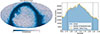 |
Fig. 1. Left: Quaia selection function. This is the basis of our masking strategy. We also show the distribution of 4520 quasars in a narrow redshift slice at 1.8 < z < 1.81 on top. Right: Redshift distribution of Quaia quasars, showing the good agreement with mocks. |
In the above observational window on the sky, we also applied a redshift cut at 0.8 < z < 2.2, leaving 708 483 quasars for our analysis, i.e. 55% of the whole quasar dataset. This choice is motivated by the higher number density of sources in the Quaia catalogue in that range (see Fig. 1), and also to allow more direct comparisons with previous results, since eBOSS quasar analyses of voids also focused on this redshift range (Kovács et al. 2022b).
2.2. Mapping the quasar density field
To estimate the local overdensity of quasars ( , where
  is the mean density) and then identify voids and clusters in their distribution, we used the open-source REVOLVER (REal-space VOid Locations from surVEy Reconstruction) code1 (Nadathur et al. 2019). Based on the ZOBOV watershed algorithm (Neyrinck 2008), REVOLVER uses a Voronoi tessellation methodology to create a detailed map of the density field (see Figs. 2 and 3 for subsets of the resulting quasar overdensity map). The algorithm first assigns a Voronoi volume to each input tracer of the large-scale structure, i.e. marking all points closer to that tracer than to any other (see vol_nocorr in Table A.2). Then, we used the optional tools in REVOLVER to apply weights for individual structures, taking into account survey completeness in pixels or in the redshift distribution (assigning a corrected volume, vol_corr), in order to correct for known imperfections in the input data.
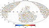 |
Fig. 2. Redshift slice of the Quaia catalogue at 1.0 < z < 1.03 in equatorial coordinates. Based on the Voronoi tessellation, the reconstructed local over-density ( |

 |
Fig. 3. Two-dimensional view of the Quaia dataset at 0.8 < z < 2.2 with −180° < RA < 180°, but only showing quasars with −0.5° < Dec < 0.5°. The over-density ( |

In the next step, the ZOBOV algorithm creates catalogues of voids and clusters from the Voronoi cells by applying the watershed approach. This is analogous to flooding a topographic land surface, where valleys get filled when water levels are rising. Then, neighbouring valleys might merge into larger basins when the water level rises further (see Neyrinck 2008, for more details). To each void and cluster, multiple features are presented as output and we listed the most relevant ones for our interests in Tables A.1 and A.2.
Here we note that we considered a flat ΛCDM cosmology using astropy2 throughout this work, including calculations of distances in the void and cluster finding processes, based on Planck Collaboration VI (2020) parameter values: H0 = 67.6 km s−1 Mpc−1, Ωm = 0.31, and ΩΛ = 0.69.
When working with REVOLVER, we pruned the Quaia input data in the following ways:
-
We used a binary sky mask to exclude pixels where completeness is low, mostly close to the Galactic plane. As mentioned in Sect. 2.1, we only kept pixels with sel_func > 0.52 completeness, leaving 24 372 deg2 of sky area. The distribution of quasars within this reliable area is depicted in Figs. 1 and 2.
-
In the rest of the sky, we used the Quaia selection function to correct the local density estimation, considering various sources of systematic effects (see Storey-Fisher et al. 2024, for details). Effectively, we increased source density by changing the Voronoi volumes of cells based on the completeness information.
-
We applied a correction based on the changing N(z) redshift distribution of sources, caused by the expected sensitivity limitation in observing quasars at higher redshifts. Technically, this step also corrects the density field reconstruction by modifying the Voronoi cell volumes based on quasar redshifts and the data sparsity at that redshift.
2.3. Mock catalogues
In this work, we use 50 mock catalogues, specifically tailored to reproduce Quaia observational data. In what follows, we briefly summarize the main features of the mocks and refer to Sinigaglia et al. (2025) for the details.
The mock catalogues used in our analysis were generated by adopting the following procedure:
-
Generation of full-sky lightcone dark matter field with smooth redshift evolution at 0 < z ≲ 4: these were obtained through the WebOn code (Sinigaglia et al. 2025), implementing the ALPT structure formation model (Kitaura & Hess 2013) directly on the lightcone;
-
Application of a non-linear, non-local, stochastic parametric Hicobian bias model (see, Coloma-Nadal et al. 2024, and references therein) to the dark matter fields to generate quasar number counts in cells. This model was first calibrated to fit the clustering of quasar halo occupation distribution mocks, reproducing the 3D clustering measurements from the DESI One-percent Survey (Yuan et al. 2024). Subsequently, the bias was fine-tuned to reproduce the angular clustering measured from Quaia data (Storey-Fisher et al. 2024). As a result, mock averages and observed clustering were in excellent, 1σ agreement level in most angular bins (see Sinigaglia et al. 2025, for more detail);
-
Application of a suited sub-grid model to assign positions and velocities to the objects: we adopt a simplified version of the sub-grid model described in Forero Sánchez et al. (2024). Specifically, we assign quasar positions in correspondence with existing dark matter particles and generate the remaining ones by means of a random uniform sampling within the cell. The velocities are modelled as in Kitaura et al. (2012a,b, 2014, 2016), Bos et al. (2019), Sinigaglia et al. (2022, 2024a,b), i.e. as the sum of a large-scale coherent flow component – consisting of the ALPT velocities – and a small-scale quasi-virialized motion accounting for the fingers-of-God.
-
Injection of Quaia observational systematics: at the last step, we assign a realistic spectrophotometric error to every quasar, sampled from the distribution measured directly from the data, and then apply both the angular and the radial selection functions, as presented in Storey-Fisher et al. (2024).
In this way, we obtained mock catalogues that closely resemble the main summary statistics from the Quaia catalogues. In particular, the angular clustering from the mock catalogues was shown to correctly reproduce the one from the data both in configuration and in Fourier space.
3. Results and deliverables
Here we present our main findings about the cosmic web traced by quasars at 0.8 < z < 2.2, and we introduce our data products, which we make publicly available for the community, making use of the cosmographical information from this analysis. Our main deliverables are the following:
-
An estimation of the local overdensity (
 ) at quasar positions in the Quaia catalogue and its mocks, based on Voronoi tessellation.
 -
The construction of void and cluster catalogues with REVOLVER, both for Quaia and its 50 mock catalogues. We note that these clusters are not expected to be virialized overdensities like galaxy clusters but instead extended groups of quasars, possibly in superclusters. We decided to refer to them as clusters to follow the generic notation of REVOLVER.
-
A value-added catalogue that contains the quasar properties from Quaia, plus the above information about the quasar’s local density and its relative position within voids or clusters.
3.1. Voids and clusters in the quasar distribution
As outlined in Section 2, the fundamental step in our cosmographical analysis of the Quaia catalogue was the estimation of the local density, based on the ZOBOV algorithm (see Figs. 2 and 3 for subsets of the density reconstruction). Then, we defined extended coherent patterns in the quasar density field as voids and clusters, and we created catalogues of such large-scale structures.
The format of these catalogues of voids and clusters in the quasar distribution is described in Table A.1. Columns include positions (RA, Dec, z), effective radius (Reff), various density parameters (expressed as δmin minima and δavg average of density fluctuation, with  ), and also a binary EdgeFlag parameter to determine if the given void or cluster is close to the edge of the survey mask. Investigating the EdgeFlag effects takes a significant part of this analysis because voids and clusters might show spurious signals where the data quality is lower near the survey mask. We note that future users of these catalogues might prune them based on their own preferences and explore the survey boundary effects. For further details about these void and cluster parameters see for example Neyrinck (2008) and Nadathur (2016).
In Figs. 4–8, we present a detailed comparison of the Quaia void and cluster catalogue parameters with the 50 mock catalogues that we analysed, given their mean and standard deviation. Each histogram shows an ∼5 − 10% level of agreement between observations and simulations, including distributions of their radii, average density, minimum or maximum density, and redshift distribution. We note that we constructed the histogram bars in such a way that voids and clusters with EdgeFlag = 1 appear on the top of the EdgeFlag = 0 part of each bar, showing their contribution to the overall count (similarly for mocks, using error bars). Here we list and explain a few characteristic features of our catalogues:
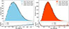 |
Fig. 4. Void radii (left) and cluster radii distribution (right) in the Quaia catalogue. With full colours, we show structures that are far from the mask (EdgeFlag = 0), while pale bars on top show the number of voids and clusters close to the survey edge (EdgeFlag = 1). We found good agreement when comparing the observations with the mean and standard deviation of the mocks (black and grey data points). On the main panels, error bars correspond to the standard deviations of the 50 mock realizations. In the bottom panels, error bars for the mocks are again estimated from the 50 realisations, while for Quaia we used the binomial sample standard deviation |
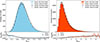 |
Fig. 5. Distributions of minimum density in void centres (left) and maximum density in cluster centres (right) in the Quaia catalogue. We again compare structures near and far from the survey edges, and also assess consistency between data and mocks. |
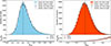 |
Fig. 6. Distributions of average density in voids (left) and average density in clusters (right) in the Quaia catalogue. We again compare structures near and far from the survey edges, and also assess consistency between data and mocks. |
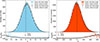 |
Fig. 7. Distributions of the λv parameter values in voids (left) and the λc parameter values in clusters (right) in the Quaia catalogue. We again compare structures near and far from the survey edges, and also assess consistency between data and mocks. |
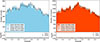 |
Fig. 8. Redshift distribution of voids (left) and clusters (right) in the Quaia catalogue. We again compare structures near and far from the survey edges, and also assess consistency between data and mocks. |
-
In total, we identified 12 820 voids and 41 154 clusters in the distribution of 708 483 quasars in Quaia, which is fully consistent with the typical yield from the mock catalogues.
-
On average, clusters are more compact than voids and their central density fluctuation is also higher (see Figs. 4 and 5).
-
Both voids and clusters are considered spherical on average but individually they might have highly irregular shapes.
-
A typical distinction between different classes of voids is voids-in-voids versus voids-in-clouds, depending on their large-scale environment. Parameters like δavg and λ provide proxies (see e.g. Raghunathan et al. 2020) for such a classification for voids, and for clusters as well (see Figs. 6 and 7).
Furthermore, we studied the level of Quaia versus mock agreement for voids and clusters located near the survey edge (EdgeFlag = 1), which might contaminate the sample due to their imperfect mapping (see Figs. 4–8). We found that:
-
the largest voids and clusters are more prone to edge effects (see tails in the bottom panels of Fig. 4). This is naturally expected, since larger structures have higher chances of touching the survey boundaries.
-
Voids with very low minimum density (δmin ≲ −0.6) and clusters with more high maximum density (δmax ≳ 2) are more sensitive to survey edge effects (see Fig. 5, and also Fig. 6 for related findings for their mean densities). The enhanced sensitivity of these structures is a result of correlations between their density and radius.
-
Considering the λ parameter, the most extreme voids and clusters show the largest fraction of edge-affected objects (see Fig. 7). This sensitivity is again due to the fact that λ is strongly correlated with the radius (see Table A.1).
-
While on average there is no significant trend in the redshift distribution of EdgeFlag = 1 in voids, we found that above z ≈ 2 their ratio slightly rises, most probably due to falling quasar number densities (see Fig. 8).
-
Overall, we report good agreement between Quaia and the mock datasets in the context of edge effects.
We highlight that this excellent agreement was not guaranteed based on the mock construction, which was mostly calibrated on the two-point correlation functions and lower-level cosmic web environment statistics. Therefore, our results further confirm the robustness of the Quaia mocks at a different level of complexity in the data analysis.
3.2. Statistics of the largest voids and clusters
The typical radius of voids is about Reff ≈ 100 h−1 Mpc, and Reff ≈ 80 h−1 Mpc for clusters. In agreement with the mock statistics, the largest voids reach Reff ≈ 250 h−1 Mpc radii, while the largest clusters are about Reff ≈ 150 h−1 Mpc in radius.
As an indicator of the sparsity of the data, the approximate mean particle separation is  Mpc at z ≈ 0.8, based on
  Mpc−3 tracer density, which increases to dmps ≈ 63 h−1 Mpc, based on a
  Mpc−3 source density at z ≈ 2.2. In turn, the usual assumption is that structures below Reff ≈ 2 ⋅ dmps are possibly spurious, and they should be excluded from the subsequent statistical analysis (see e.g. Hamaus et al. 2016). These structures are nevertheless present in our output catalogues, for the sake of completeness, and we leave it to future users to implement the desired pruning cuts that are suitable for their concrete applications.
Considering the high-end tail of the void and cluster radius distribution (see Fig. 4), we again note that the largest structures are most prone to contamination from masking effects, and only the clean EdgeFlag = 0 subset should be considered for statistical analyses. All things considered, we did not find any evidence of outstanding, ultra-large quasar groups or giant empty voids, neither in the Quaia quasar distribution, nor in its 50 mock catalogues. This conclusion was also strengthened by visual inspection using different redshift bins and wedges in the data, in the spirit of Figs. 2 and 3. We leave the more detailed and formal statistical analysis of the largest structures for future work.
3.3. A value-added quasar catalogue
With the intention to create a value-added catalogue of quasars, we combined the information on the local density at quasar positions with the quasar’s relative position within voids or clusters. This is relevant because  itself is not a unique indicator of void or cluster membership and large-scale environment. We note that there are deeper and shallower voids in the catalogue (based on δavg and λ) where a quasar with a given density might be located near the void’s centre or at its outskirts close to its compensation wall (for more information about void types and the role of their environment, see e.g. Raghunathan et al. 2020).
This combined dataset is presented in Table A.2, with the following information in three subsections:
-
First, we listed the main outputs from the tessellation: raw Voronoi volume around the quasar, corrected Voronoi volume (based on selection functions), normalized density (1/Vcorr), Gaia source ID, unWISE object ID, the selection function value at the position of the quasar, and a quality flag.
-
The bottom two sections of Table A.2 contain information about the host void and/or cluster of the given quasar, listing the most important void and cluster parameters that we also provide in Table A.1 (REVOLVER allows for a quasar to be both a member of a void and a cluster, as these catalogues are constructed in two separate watershed runs on the data).
-
Based on additional information on membership in voids and clusters provided by REVOLVER, we calculated the R/Reffrelative position of each quasar in its host structure, labelled as R_over_Rv for voids and R_over_Rc for clusters.
-
For voids, we provide coordinates both circumcentre (defined by the quasar with the most extreme density and its neighbouring cells near the centre) and barycentre definitions, while for clusters we only provide circumcentres given REVOLVER’s default setting.
The extensive list of columns is intended to help future users make elaborate cuts in the data for their own purposes. One may filter this value-added quasar catalogue by local quasar density, data quality given the selection function at the quasar’s pixel, redshift of the quasar, or the radius of the host void or cluster to which the quasar belongs; this can lead to various applications. In particular, the radio loudness of quasars and its dependence on local density might also be studied (see e.g. Arsenov et al. 2025) as yet another application of the Quaia catalogue.
3.4. Density profiles of voids and clusters
To further characterize our void and cluster catalogues, we also measured their quasar number density profiles, again in comparison with the mocks. As we noted above, the Quaia catalogue is rather sparse, with  Mpc−3, which limits our capacity to provide a detailed reconstruction of the true underlying matter density field. However, the large number of voids (Nv = 12 820) and clusters (Nc = 41 154) in our sample allows us to provide a precise measurement of the stacked density profile for tens of thousands of cosmic superstructures, which further probes the consistency between simulations and observations.
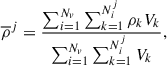
We decided to use the Voronoi tessellation field estimator (VTFE) method to calculate the density profiles, as opposed to cruder counts-in-shells estimates, which are more prone to Poisson noise (see e.g. Nadathur et al. 2014). This is a typical choice when using void and cluster catalogues detected with the ZOBOV methodology. We used the following volume-weighted estimator for the stacked density in the jth radial shell from the void or cluster centre, which makes use of the VTFE reconstructed density information:
 (1)
(1)
where Vk is the volume of the Voronoi cell of the quasar k and ρk is its density inferred from the inverse of the Voronoi volume; the sum over k runs over all quasars in the jth shell of void or cluster i (not only void or cluster member quasars); and the sum over i includes all voids or clusters (Nv or Nc) in the stack. We used 25 radial bins up to R/Rv = 3 to measure the shapes of the density profiles in sufficient detail.
Our findings are presented in Fig. 9, including a detailed comparison between density profiles measured from Quaia versus the mean and standard deviation of the 50 mock catalogues. As in previous figures, we also compared EdgeFlag = 0 and EdgeFlag = 1 cases for both voids and clusters. We then further explored the data by splitting the catalogues on the λ parameter, isolating subsets of voids-in-voids (λ < −40) and voids-in-clouds (λ > 40) and similar subsets for clusters in dominantly under-dense and over-dense environments. We confirm the robustness of our mapping of high-z cosmic web using the Quaia quasars, as well as using its realistic mock catalogues, by drawing the following conclusions:
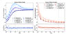 |
Fig. 9. Density profiles of voids (left) and clusters (right) in the Quaia catalogue. We again compare structures near and far from the survey edges, and also assess consistency between data (Q) and mocks (M) in the bottom panels. We show the density profiles using all voids and clusters, and we also split the catalogues into subsets with extreme values of λv and λc, as a proxy for their environment. |
-
In spite of the sparse quasar distribution, we find rather smooth and significantly under-dense profiles for voids, and over-dense profiles for clusters.
-
The agreement between Quaia and the mocks is excellent (approx. 5 − 10%), both for voids and clusters.
-
As expected, EdgeFlag = 1 voids and clusters show more noisy and somewhat distorted profiles compared to the clean EdgeFlag = 0 subset. However, the agreement between mocks and data remains excellent in this aspect as well.
-
We found a clear separation between subsets of voids and clusters, selected with different λ parameter cuts.
4. Summary and conclusions
In this cosmographical analysis, we took the Quaia catalogue of quasars as an input and mapped the cosmic web at redshifts 0.8 < z < 2.2. While quasar catalogues only allow a rather sparse sampling of the underlying matter distribution, our motivation was to go beyond the current state-of-the-art in high-z void finding in the quasar distribution (see Aubert et al. 2022; Kovács et al. 2022b, for eBOSS DR16 results). We thus created a value-added dataset for the 708 483 quasars that we analysed, and our main analysis steps were the following:
-
Taking into account survey systematics through selection functions (quasar redshift distribution, completeness in pixels), we used the REVOLVER algorithm to estimate the local density at the positions of the quasars (see Figs. 2 and 3).
-
We then built a catalogue of 12 820 voids and 41 154 clusters in the Quaia quasar distribution based on a Voronoi tessellation algorithm, using 24 372 deg2 of the sky area.
-
Importantly, we compared our observational results with 50 mock catalogues, in terms of void and cluster radii, mean, minimum and maximum densities, and redshift distribution, finding an excellent ∼5 − 10% level of agreement (see Figs. 4–8).
-
For completeness, we estimated the density profiles of the voids and clusters in our catalogue, again comparing observational and synthetic data. For different subsets based on edge effects and void or cluster environments, we again found good agreement (see Fig. 9).
The final deliverable of our work is a combination of the local density estimation ( ) with the information about the membership of Quaia quasars in voids and clusters (Reff, δmin, λv etc.). This way, it becomes possible to label the quasars based on either of these cosmic web environment parameters, or their combinations, and thus create subsets that are located in over-dense or under-dense environments, even specifying their relative positions within voids (R/Rv) or clusters (R/Rc).
We foresee various applications, including cross-correlations with CMB maps, radio catalogues, or data at other wavelengths, which motivates the public release of our value-added catalogues. This dataset will contribute to the full exploitation of the Quaia quasar catalogue in even greater detail in terms of cosmic web mapping at high redshift.
Data availability
The Quaia quasar catalogue and the corresponding selection function map are made publicly available3 by their authors (Storey-Fisher et al. 2024). The REVOLVER code is also available publicly4, with documentation and examples to run it on synthetic or observational data sets. The main products from this work, presented in Tables A.1 and A.2 are available at the CDS via https://cdsarc.cds.unistra.fr/viz-bin/cat/J/A+A/706/A362. Code for reproducing our analysis and figures is publicly available at https://doi.org/10.5281/zenodo.16359456. We are available for consultation about the results or our methodology.
Acknowledgments
The Large-Scale Structure (LSS) research group at Konkoly Observatory has been supported by a Lendület excellence grant by the Hungarian Academy of Sciences (MTA). This project has received funding from the European Union’s Horizon Europe research and innovation programme under the Marie Skłodowska-Curie grant agreement number 101130774. Funding for this project was also available in part through the Hungarian National Research, Development and Innovation Office (NKFIH, grant OTKA NN147550). L.S.-M. was partially supported by the Bulgarian Ministry of Education and Science under Agreement D01-326/04.12.2023. The authors thank Kate Storey-Fisher and the Quaia team for their help with the input quasar catalogue.
References
- Alonso, D., Hill, J. C., Hložek, R., & Spergel, D. N. 2018, Phys. Rev. D, 97, 063514 [NASA ADS] [CrossRef] [Google Scholar]
- Alonso, D., Hetmantsev, O., Fabbian, G., Slosar, A., & Storey-Fisher, K. 2025, Open J. Astrophys., 8, 42 [Google Scholar]
- Amendola, L., Frieman, J. A., & Waga, I. 1999, MNRAS, 309, 465 [NASA ADS] [CrossRef] [Google Scholar]
- Amendola, L., Appleby, S., Bacon, D., et al. 2013, Liv. Rev. Relat., 16, 6 [Google Scholar]
- Arsenov, N., Frey, S., Kovács, A., & Slavcheva-Mihova, L. 2025, ApJS, 280, 23 [Google Scholar]
- Aubert, M., Cousinou, M.-C., Escoffier, S., et al. 2022, MNRAS, 513, 186 [NASA ADS] [CrossRef] [Google Scholar]
- Baker, T., Clampitt, J., Jain, B., & Trodden, M. 2018, Phys. Rev. D, 98, 023511 [NASA ADS] [CrossRef] [Google Scholar]
- Bos, E. G. P., Kitaura, F.-S., & van de Weygaert, R. 2019, MNRAS, 488, 2573 [NASA ADS] [CrossRef] [Google Scholar]
- Cai, Y.-C., Cole, S., Jenkins, A., & Frenk, C. 2009, MNRAS, 396, 772 [Google Scholar]
- Cai, T., Fan, J., & Jiang, T. 2013, Technical Report of the Department of Statistics, University of Pennsylvania [Google Scholar]
- Cai, Y.-C., Padilla, N., & Li, B. 2015, MNRAS, 451, 1036 [NASA ADS] [CrossRef] [Google Scholar]
- Camacho-Ciurana, G., Lee, P., Arsenov, N., et al. 2024, A&A, 689, A171 [NASA ADS] [CrossRef] [EDP Sciences] [Google Scholar]
- Cautun, M., Paillas, E., Cai, Y.-C., et al. 2018, MNRAS, 476, 3195 [NASA ADS] [CrossRef] [Google Scholar]
- Clampitt, J., Cai, Y.-C., & Li, B. 2013, MNRAS, 431, 749 [NASA ADS] [CrossRef] [Google Scholar]
- Clowes, R. G., Raghunathan, S., Harris, K. A., et al. 2014, Rev. Mex. Astron. Astrofis. Conf. Ser., 44, 201 [Google Scholar]
- Coloma-Nadal, J. M., Kitaura, F. S., García-Farieta, J. E., et al. 2024, JCAP, 2024, 083 [CrossRef] [Google Scholar]
- Contarini, S., Marulli, F., Moscardini, L., et al. 2021, MNRAS, 504, 5021 [NASA ADS] [CrossRef] [Google Scholar]
- Davies, C. T., Cautun, M., Giblin, B., et al. 2021, MNRAS, 507, 2267 [NASA ADS] [Google Scholar]
- Delchambre, L., Bailer-Jones, C. A. L., Bellas-Velidis, I., et al. 2023, A&A, 674, A31 [NASA ADS] [CrossRef] [EDP Sciences] [Google Scholar]
- Douglass, K. A., Veyrat, D., & BenZvi, S. 2023, ApJS, 265, 7 [NASA ADS] [CrossRef] [Google Scholar]
- Einasto, J., Hütsi, G., Suhhonenko, I., Liivamägi, L. J., & Einasto, M. 2021, A&A, 647, A17 [NASA ADS] [CrossRef] [EDP Sciences] [Google Scholar]
- Fabbian, G., Alonso, D., Storey-Fisher, K., & Cornish, T. 2025, ArXiv e-prints [arXiv:2504.20992] [Google Scholar]
- Fang, Y., Hamaus, N., Jain, B., Pandey, S., & DES Collaboration 2019, MNRAS, 490, 3573 [NASA ADS] [CrossRef] [Google Scholar]
- Forero Sánchez, D., Kitaura, F. S., Sinigaglia, F., Coloma-Nadal, J. M., & Kneib, J. P. 2024, JCAP, 2024, 001 [Google Scholar]
- Gaia Collaboration (Bailer-Jones, C. A. L., et al.) 2023a, A&A, 674, A41 [NASA ADS] [CrossRef] [EDP Sciences] [Google Scholar]
- Gaia Collaboration (Vallenari, A., et al.) 2023b, A&A, 674, A1 [NASA ADS] [CrossRef] [EDP Sciences] [Google Scholar]
- Gorski, K. M., Hivon, E., Banday, A. J., et al. 2005, ApJ, 622, 759 [Google Scholar]
- Granett, B. R., Neyrinck, M. C., & Szapudi, I. 2008, ApJ, 683, L99 [NASA ADS] [CrossRef] [Google Scholar]
- Hamaus, N., Pisani, A., Sutter, P. M., et al. 2016, Phys. Rev. Lett., 117, 091302 [NASA ADS] [CrossRef] [Google Scholar]
- Hamaus, N., Aubert, M., Pisani, A., et al. 2021, A&A, 658, A20 [Google Scholar]
- Hawken, A. J., Granett, B. R., Iovino, A., et al. 2017, A&A, 607, A54 [NASA ADS] [CrossRef] [EDP Sciences] [Google Scholar]
- Horvath, I., Bagoly, Z., Balazs, L. G., et al. 2025, Universe, 11, 121 [Google Scholar]
- Ilić, S., Langer, M., & Douspis, M. 2013, A&A, 556, A51 [NASA ADS] [CrossRef] [EDP Sciences] [Google Scholar]
- Kitaura, F. S., & Hess, S. 2013, MNRAS, 435, L78 [NASA ADS] [CrossRef] [Google Scholar]
- Kitaura, F.-S., Erdoǧdu, P., Nuza, S. E., et al. 2012a, MNRAS, 427, L35 [NASA ADS] [Google Scholar]
- Kitaura, F.-S., Gallerani, S., & Ferrara, A. 2012b, MNRAS, 420, 61 [Google Scholar]
- Kitaura, F. S., Yepes, G., & Prada, F. 2014, MNRAS, 439, L21 [NASA ADS] [CrossRef] [Google Scholar]
- Kitaura, F.-S., Ata, M., Angulo, R. E., et al. 2016, MNRAS, 457, L113 [Google Scholar]
- Kovács, A., Sánchez, C., García-Bellido, J., & the DES Collaboration 2017, MNRAS, 465, 4166 [CrossRef] [Google Scholar]
- Kovács, A., Sánchez, C., García-Bellido, J., & the DES Collaboration 2019, MNRAS, 484, 5267 [CrossRef] [Google Scholar]
- Kovács, A., Jeffrey, N., Gatti, M., et al. 2022a, MNRAS, 510, 216 [Google Scholar]
- Kovács, A., Beck, R., Smith, A., et al. 2022b, MNRAS, 513, 15 [CrossRef] [Google Scholar]
- Krause, E., Chang, T.-C., Doré, O., & Umetsu, K. 2013, ApJ, 762, L20 [NASA ADS] [CrossRef] [Google Scholar]
- Lang, D. 2014, AJ, 147, 108 [Google Scholar]
- Levi, M., Bebek, C., Beers, T., et al. 2013, ArXiv e-prints [arXiv:1308.0847] [Google Scholar]
- Li, G., Ma, Y.-Z., Tramonte, D., & Li, G.-L. 2024, MNRAS, 527, 2663 [Google Scholar]
- Libeskind, N. I., van de Weygaert, R., Cautun, M., et al. 2018, MNRAS, 473, 1195 [NASA ADS] [CrossRef] [Google Scholar]
- Liu, A., Bulbul, E., Kluge, M., et al. 2024, A&A, 683, A130 [NASA ADS] [CrossRef] [EDP Sciences] [Google Scholar]
- Lopez, A. M., Clowes, R. G., & Williger, G. M. 2022, MNRAS, 516, 1557 [Google Scholar]
- LSST Science Collaboration (Abell, P. A., et al.) 2009, ArXiv e-prints [arXiv:0912.0201] [Google Scholar]
- Mao, Q., Berlind, A. A., Scherrer, R. J., et al. 2017, ApJ, 835, 161 [NASA ADS] [CrossRef] [Google Scholar]
- Nadathur, S. 2013, MNRAS, 434, 398 [Google Scholar]
- Nadathur, S. 2016, MNRAS, 461, 358 [NASA ADS] [CrossRef] [Google Scholar]
- Nadathur, S., & Crittenden, R. 2016, ApJ, 830, L19 [CrossRef] [Google Scholar]
- Nadathur, S., Lavinto, M., Hotchkiss, S., & Räsänen, S. 2014, Phys. Rev. D, 90, 103510 [NASA ADS] [CrossRef] [Google Scholar]
- Nadathur, S., Carter, P. M., Percival, W. J., Winther, H. A., & Bautista, J. E. 2019, Phys. Rev. D, 100, 023504 [CrossRef] [Google Scholar]
- Naidoo, K., Whiteway, L., Massara, E., et al. 2020, MNRAS, 491, 1709 [NASA ADS] [CrossRef] [Google Scholar]
- Neyrinck, M. C. 2008, MNRAS, 386, 2101 [CrossRef] [Google Scholar]
- Park, C., Song, H., Einasto, M., Lietzen, H., & Heinamaki, P. 2015, JKAS, 48, 75 [Google Scholar]
- Piccirilli, G., Fabbian, G., Alonso, D., et al. 2024, JCAP, 2024, 012 [Google Scholar]
- Pisani, A., Sutter, P. M., Hamaus, N., et al. 2015, Phys. Rev. D, 92, 083531 [NASA ADS] [CrossRef] [Google Scholar]
- Pisani, A., Massara, E., Spergel, D. N., et al. 2019, BAAS, 51, 40 [Google Scholar]
- Planck Collaboration VI. 2020, A&A, 641, A6 [NASA ADS] [CrossRef] [EDP Sciences] [Google Scholar]
- Potter, D., Stadel, J., & Teyssier, R. 2016, ArXiv e-prints [arXiv:1609.08621] [Google Scholar]
- Rácz, G., Kiessling, A., Csabai, I., & Szapudi, I. 2023, A&A, 672, A59 [NASA ADS] [CrossRef] [EDP Sciences] [Google Scholar]
- Raghunathan, S., Nadathur, S., Sherwin, B. D., & Whitehorn, N. 2020, ApJ, 890, 168 [NASA ADS] [CrossRef] [Google Scholar]
- Rincon, H., Benzvi, S., Douglass, K., et al. 2025, ApJ, 982, 38 [Google Scholar]
- Sachs, R. K., & Wolfe, A. M. 1967, ApJ, 147, 73 [NASA ADS] [CrossRef] [Google Scholar]
- Sánchez, C., Clampitt, J., Kovács, A., et al. 2017, MNRAS, 465, 746 [CrossRef] [Google Scholar]
- Sartori, S., Vielzeuf, P., Escoffier, S., et al. 2025, A&A, 700, A17 [NASA ADS] [CrossRef] [EDP Sciences] [Google Scholar]
- Sawala, T., Teeriaho, M., Frenk, C. S., et al. 2025, MNRAS, 541, L22 [Google Scholar]
- Schaye, J., Kugel, R., Schaller, M., et al. 2023, MNRAS, 526, 4978 [NASA ADS] [CrossRef] [Google Scholar]
- Schuster, N., Hamaus, N., Pisani, A., et al. 2019, JCAP, 2019, 055 [Google Scholar]
- Sinigaglia, F., Kitaura, F.-S., Balaguera-Antolínez, A., et al. 2022, ApJ, 927, 230 [NASA ADS] [CrossRef] [Google Scholar]
- Sinigaglia, F., Kitaura, F.-S., Nagamine, K., & Oku, Y. 2024a, ApJ, 971, L22 [Google Scholar]
- Sinigaglia, F., Kitaura, F. S., Nagamine, K., Oku, Y., & Balaguera-Antolínez, A. 2024b, A&A, 682, A21 [NASA ADS] [CrossRef] [EDP Sciences] [Google Scholar]
- Sinigaglia, F., Kitaura, F. S., Shiferaw, M., et al. 2025, ArXiv e-prints [arXiv:2509.15890] [Google Scholar]
- Storey-Fisher, K., Hogg, D. W., Rix, H.-W., et al. 2024, ApJ, 964, 69 [NASA ADS] [CrossRef] [Google Scholar]
- Takahashi, R., Hamana, T., Shirasaki, M., et al. 2017, ApJ, 850, 24 [Google Scholar]
- The Dark Energy Survey Collaboration 2005, ArXiv e-prints [arXiv:astro-ph/0510346] [Google Scholar]
- Veronesi, N., van Velzen, S., Rossi, E. M., & Storey-Fisher, K. 2025, MNRAS, 536, 375 [Google Scholar]
- Vielzeuf, P., Calabrese, M., Carbone, C., Fabbian, G., & Baccigalupi, C. 2023, JCAP, 2023, 010 [CrossRef] [Google Scholar]
- Yuan, S., Zhang, H., Ross, A. J., et al. 2024, MNRAS, 530, 947 [CrossRef] [Google Scholar]
Appendix A: Data Tables
Properties of the Quaia void and cluster catalogues.
Value-added catalogue for all Quaia quasars in our analysis
All Tables
All Figures
|
Fig. 1. Left: Quaia selection function. This is the basis of our masking strategy. We also show the distribution of 4520 quasars in a narrow redshift slice at 1.8 < z < 1.81 on top. Right: Redshift distribution of Quaia quasars, showing the good agreement with mocks. |
| In the text | |
|
Fig. 2. Redshift slice of the Quaia catalogue at 1.0 < z < 1.03 in equatorial coordinates. Based on the Voronoi tessellation, the reconstructed local over-density ( |
| In the text | |
|
Fig. 3. Two-dimensional view of the Quaia dataset at 0.8 < z < 2.2 with −180° < RA < 180°, but only showing quasars with −0.5° < Dec < 0.5°. The over-density ( |
| In the text | |
|
Fig. 4. Void radii (left) and cluster radii distribution (right) in the Quaia catalogue. With full colours, we show structures that are far from the mask (EdgeFlag = 0), while pale bars on top show the number of voids and clusters close to the survey edge (EdgeFlag = 1). We found good agreement when comparing the observations with the mean and standard deviation of the mocks (black and grey data points). On the main panels, error bars correspond to the standard deviations of the 50 mock realizations. In the bottom panels, error bars for the mocks are again estimated from the 50 realisations, while for Quaia we used the binomial sample standard deviation |
| In the text | |
|
Fig. 5. Distributions of minimum density in void centres (left) and maximum density in cluster centres (right) in the Quaia catalogue. We again compare structures near and far from the survey edges, and also assess consistency between data and mocks. |
| In the text | |
|
Fig. 6. Distributions of average density in voids (left) and average density in clusters (right) in the Quaia catalogue. We again compare structures near and far from the survey edges, and also assess consistency between data and mocks. |
| In the text | |
|
Fig. 7. Distributions of the λv parameter values in voids (left) and the λc parameter values in clusters (right) in the Quaia catalogue. We again compare structures near and far from the survey edges, and also assess consistency between data and mocks. |
| In the text | |
|
Fig. 8. Redshift distribution of voids (left) and clusters (right) in the Quaia catalogue. We again compare structures near and far from the survey edges, and also assess consistency between data and mocks. |
| In the text | |
|
Fig. 9. Density profiles of voids (left) and clusters (right) in the Quaia catalogue. We again compare structures near and far from the survey edges, and also assess consistency between data (Q) and mocks (M) in the bottom panels. We show the density profiles using all voids and clusters, and we also split the catalogues into subsets with extreme values of λv and λc, as a proxy for their environment. |
| In the text | |
Current usage metrics show cumulative count of Article Views (full-text article views including HTML views, PDF and ePub downloads, according to the available data) and Abstracts Views on Vision4Press platform.
Data correspond to usage on the plateform after 2015. The current usage metrics is available 48-96 hours after online publication and is updated daily on week days.
Initial download of the metrics may take a while.