| Issue |
A&A
Volume 706, February 2026
|
|
|---|---|---|
| Article Number | A210 | |
| Number of page(s) | 19 | |
| Section | Galactic structure, stellar clusters and populations | |
| DOI | https://doi.org/10.1051/0004-6361/202557533 | |
| Published online | 16 February 2026 | |
Kinematics of young stellar objects in NGC 2024 based on infrared proper motions
1
Department of Astrophysics, University of Vienna,
Türkenschanzstrasse 17,
1180
Wien,
Austria
2
European Southern Observatory,
Karl-Schwarzschild-Strasse 2,
85748
Garching bei München,
Germany
3
University of Vienna, Research Network Data Science at Uni Vienna,
Kolingasse 14-16,
1090
Wien,
Austria
4
Université Paris-Saclay, Université Paris Cité, CEA, CNRS, AIM,
91191
Gif-sur-Yvette,
France
5
Laboratoire d’astrophysique de Bordeaux, Univ. Bordeaux, CNRS, B18N, allée Geoffroy Saint-Hilaire,
33615
Pessac,
France
6
Institut universitaire de France (IUF),
1 rue Descartes,
75231
Paris Cedex 05,
France
7
Center for Astrophysics | Harvard & Smithsonian,
60 Garden St.,
Cambridge,
MA
02138,
USA
★ Corresponding author: This email address is being protected from spambots. You need JavaScript enabled to view it.
Received:
2
October
2025
Accepted:
27
November
2025
Abstract
The most recently formed young stellar objects (YSOs) in active star-forming regions are excellent tracers of their parent cloud motion. Their positions and dynamics provide insights into cluster formation and constrain kinematic decoupling timescales between stars and gas. However, because of their strong extinction and young age, embedded YSOs are mainly visible at infrared wavelengths, and are thus absent from astrometric surveys such as Gaia. We measured the proper motions of 6769 sources toward the NGC 2024 cluster in the Flame Nebula (d ~ 420 pc) using multi-epoch near-infrared observations from three ESO public surveys: VISIONS, VHS, and the VISTA/VIRCAM science verification program. Cross-validation of our results with Gaia using optically visible stars shows excellent agreement, with uncertainties on the same order of magnitude. For 362 YSO candidates identified from the literature, we derived proper motions on the order of <5 mas yr−1 with mean measurement uncertainties of 0.22 mas yr−1, or 0.44 km s−1. This is the first homogeneous proper motion measurement of this quality for more than half of these stars. For Class I and flat-spectrum sources, our results provide a >13-fold increase in available proper motion measurements. We analyzed the positional and kinematic differences between YSO classes and confirmed a previously reported inside-out age segregation from younger to older stars, likely driven by an outward movement of older stars. No evidence of prolonged hierarchical assembly was found. Instead, the results support a rapid (<1 Myr) cluster collapse into a centrally concentrated system. This scenario also accounts for the observed slightly higher 1D velocity dispersion of Class I sources relative to Class flat objects. YSO radial velocities generally align with the gas velocities measured from the molecular transitions of 12CO(3 − 2), HNC(1 − 0), HCN(1 − 0), and show a weaker correlation with N2H+(1 − 0). Some Class II and III objects already appear to be decoupling.
Key words: proper motions / stars: kinematics and dynamics / stars: pre-main sequence / open clusters and associations: individual: Orion
© The Authors 2026
 Open Access article, published by EDP Sciences, under the terms of the Creative Commons Attribution License (https://creativecommons.org/licenses/by/4.0), which permits unrestricted use, distribution, and reproduction in any medium, provided the original work is properly cited.
This article is published in open access under the Subscribe to Open model. This email address is being protected from spambots. You need JavaScript enabled to view it. to support open access publication.
1 Introduction
Star formation is one of the most-studied processes in the field of astronomy. Its physical drivers and relative timelines set the initial conditions of planet formation and habitability (e.g., Dai et al. 2023) and can shape enormous Galactic structures (e.g., Alves et al. 2020; Swiggum et al. 2024). It is understood that many stars form simultaneously (Lada & Lada 2003) from a complex network of dense filaments and hubs (e.g., Myers 2009; André et al. 2010; Kumar et al. 2020). As the filaments fragment and collapse to form pre-stellar cores and later young stellar objects (YSOs), they imprint their structural and kinematic properties on the newly formed objects (Hacar et al. 2016).
However, the formation process of star clusters remains debated. Simulations suggest a hierarchical merging of subclusters at early times, but soon after their structure can resemble monolithic growth (Laverde-Villarreal et al. 2025, and references therein). Recent simulations found that initially hierarchical spatial substructure dissipated within ≤2.5 freefall times, but kinematic signatures persisted longer (Laverde-Villarreal et al. 2025). In contrast, simulations by Sills et al. (2018), with initial parameters inspired by observations (Kuhn et al. 2019), showed a rapid cluster collapse of ≤ 1 Myr into a monolithic system without any detectable substructure. The collapse scenarios were also shown to change YSO velocity dispersions as a function of their age (e.g., Proszkow et al. 2009; Sills et al. 2018).
The different formation pathways of clusters demonstrate that simulations strongly depend on the initial conditions and relative timescales of star formation, which are themselves poorly constrained. YSOs are born with a physical memory of their birth cloudlet that - unless the gas still present was recently disturbed by feedback, shocks, or winds - traces the motion of the surrounding material. Over the span of a few 105 - 106 yr, YSOs decouple kinematically and spatially from the gas. This process is likely partly driven by N-body interactions increasing the stellar velocity dispersion (Bate et al. 2003). At the same time, the gas reservoir gets diminished by both star formation and dispersal by stellar feedback. The timescales of the decoupling remain poorly constrained, making them one of the central open problems in star formation. They are not only essential for understanding the relative roles of stellar feedback, the dynamical state and stability of clusters, and the molecular cloud lifetimes, but are also critical for the initial conditions of simulations (Laverde-Villarreal et al. 2025).
At present, observations are the only available method of constraining decoupling timescales and testing cluster assembly theories. In this respect, the Gaia (Prusti et al. 2016) has dramatically advanced our dynamical understanding of star formation, providing five- or six-dimensional position-velocity data (α, δ, ϖ, μα*, μδ, vLOS) for over a billion sources (Vallenari et al. 2023). These data have revealed feedback-driven structures and evolutionary timescales of star-forming complexes that are a few million years old (Ratzenböck et al. 2023; Posch et al. 2023, 2025). However, as an optical instrument, Gaia cannot probe the crucial first few million years of star formation. stellar nurseries are sites of a phase transition between diffuse gas and compact YSOs, often heavily obscured by dust. Newly formed stars are embedded in high column density regions and surrounded by circumstellar disks that absorb and re-emit radiation at longer wavelengths. Thus, they are optically obscured, but readily detectable from the infrared to the radio regime, depending on their extinction and evolutionary stage. This means that precise and homogeneous kinematic measurements such as those provided by Gaia are still lacking for young (1-5 Myr) populations with embedded components.
With this project, we propose a complementary method to Gaia to address this gap: Accessing the kinematics of embedded YSOs in a young cluster using ground-based multi-epoch infrared observations.
We focused on the NGC 2024 cluster in Orion B (d ≈ 420 pc, Kounkel et al. 2017a; Zucker et al. 2019; Cao et al. 2023), the second most massive active stellar nursery in the Orion molecular cloud complex. It is embedded in the Flame Nebula, an extensive H II region extending around a central dark lane with a pronounced molecular ridge in the N-S direction, which absorbs light from the visible to the near infrared (NIR) range (Meyer et al. 2008, and references therein). The age estimates for the cluster generally fall below 0.5-2 Myr (Meyer 1996; Levine et al. 2006; Getman et al. 2014a), with ongoing star formation still suspected in its central regions (Skinner et al. 2003). Evidence suggests a radial age gradient increasing from 0.2 Myr in the core to ~1.5 Myr at a distance of ~1 pc from the center (Getman et al. 2014a). NGC 2024 consists of several hundred stars (e.g., Kounkel et al. 2017b, ≈475 Class 0/I and II YSOs), identified primarily via photometric surveys and infrared excess measurements (e.g., Meyer 1996) or X-rays (Getman et al. 2014a). The majority of photometrically detected cluster members appear to be harboring accretion disks (e.g., Skinner et al. 2003; van Terwisga et al. 2020). Attempts to determine cluster members via positional and kinematic Gaia data yielded only a fraction (30-60 stars) of the estimated cluster census (e.g., Kounkel et al. 2017b; Zerjal et al. 2024). Its many embedded members and large kinematic dispersion (Zerjal et al. 2024) likely contribute to the cluster’s absence in the Unified Cluster Catalog (Perren et al. 2023), which summarizes recent clustering efforts.
In this work, we calculated infrared-based proper motions of the same astrometric quality as Gaia for 6769 sources in the direction of the Flame Nebula, among them 362 YSO candidates. Based on this new kinematic information, we discuss different cluster formation scenarios for NGC 2024 and find the bestfitting one to be a rapid (<1 Myr) collapse of any substructure into monolithic conditions. We see an overall good agreement between YSO and gas radial velocities, indicating no significant kinematic decoupling except for some older YSOs.
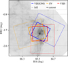 |
Fig. 1 Outlines of the SV, VHS, and VISIONS tiles covering the Flame Nebula, plotted over the Herschel Gould Belt Survey 350 μm emission map. The bold squares show the cutouts used in this study. The varying tile orientations result from the survey-specific observing strategies. |
2 Data
Calculating proper motions of embedded stars d ~ 400 pc requires observations in infrared passbands with a large temporal baseline and high positional accuracy. For reference, uncertainties in proper motion of 1 mas yr−1 correspond to physical uncertainties of around 2 km s−1 at this distance. For homogeneity of the results, using the same instrumental setup for all observations is ideal. Wide-field near-infrared surveys are well suited for obtaining spatially complete samples of embedded populations in nearby star-forming regions (e.g., Großschedl et al. 2019).
We use data from three ESO public surveys carried out with the VISTA/VIRCAM instrument: The Science Verification Galactic mini-survey of Orion (PI: Monika Petr-Gotzens, Arnaboldi et al. 2010; Petr-Gotzens et al. 2011, ESO program ID 60.A-9285), hereafter called SV, the Vista Hemisphere Survey (PI: Richard McMahon, McMahon et al. 2013, ESO program ID 179.A2010), hereafter called VHS, and the VISIONS survey (PI João Alves, Meingast et al. 2023a, ESO program ID 198.C-2009). The SV survey provides one epoch of observations in the J, H, and Ks bands from October 2009, while VHS contributes an epoch in the J and Ks bands from November 2014. VISIONS adds six H-band epochs between 2017 and 2020. Combined, the 11 datasets provide a temporal baseline of ≈10.3 years.
The Flame Nebula is located within a single ~1.5° × 1.0° “tile” (see Appendix C) in each survey. Figure 1 shows the tile locations plotted on the Herschel Gould Belt survey 350 μm map1 of Orion B (André et al. 2010; Arzoumanian et al. 2019; Könyves et al. 2020). For our study, we focused on 0.77° × 0.77° cutouts centered on the Flame Nebula, corresponding to an area of around 29 pc2 at d ~ 420 pc. The observing parameters for all datasets are listed in Table C.1.
2.1 Science Verification Galactic mini-survey
The SV galactic-mini survey (Arnaboldi et al. 2010; Petr-Gotzens et al. 2011) is a multi-wavelength, high-sensitivity survey of the Orion belt, Orion B, and σ Ori populations with a focus on studying the low-mass end of the initial mass function, searching protostellar disks, and investigating photometric variability in low-mass objects. The observations took place between October 15 and November 2, 2009, and consist of 20 tiles covering an area of about 30 deg2 around the belt stars.
The tiles were captured with a 15° tilt in position angle relative to North. The field was observed in the broadband filters ZYJHKs, split into two observation blocks that were carried out in immediate succession for each tile. As the main survey objective was to study low-mass objects, its exposure times are longer than those of VISIONS or the VHS, using 8-12 detector integrations of 2-4 s per readout. Two jitters were performed at each pawprint position. The 5σ sensitivity limits of the survey were reported as Z = 22.5 mag, Y = 21.2 mag, J = 20.4 mag, H = 19.4 mag, and Ks = 18.6 mag (Petr-Gotzens et al. 2011). Further details about the observing strategy are given in Arnaboldi et al. (2010). The Flame Nebula is located on tile 4 of the survey.
2.2 Vista Hemisphere Survey
The VHS (McMahon et al. 2013) is a Cycle 1 program of VISTA2, which mapped the entire southern hemisphere (Declination <0°) between 2010 and 2022. The observations were taken in the J and Ks passbands, with a reported median 5σ sensitivity limit of J = 20.2 mag and Ks = 18.1 mag. The most recent VHS data release, DR53, covers around 16 730 square degrees of the southern sky in at least one passband and covers the time frame between November 2009 and March 2017.
The VHS tiles have a rotator-sky angle of 180°, such that each tile covers about 1.5° in Right Ascension (RA, α) and 1° in Declination (DEC, δ). They were captured with an effective exposure time texp = 60 s, with long single exposure times and two jitter positions, similar to the SV survey. The Flame Nebula is located on tile 1_1_15 in the VHS Stripe 02. The tile was observed during ESO period 94 in November 2014, adding an intermittent data point for proper motion calculations between the SV and VISIONS observations.
2.3 VISIONS
VISIONS (Meingast et al. 2023a) is a VISTA Cycle 2 public survey (Arnaboldi et al. 2019) designed to produce highly accurate multi-epoch position measurements and proper motions for nearby (d < 500 pc) star-forming complexes. It primarily covers low-mass, embedded objects with no Gaia coverage. It includes the five nearby regions Chamaeleon, Corona Australis, Lupus, Ophiuchus, and Orion, comprising 650 deg2 of the night sky with roughly 50 h total exposure time. The observations of all regions were taken between April 2017 and March 2022.
VISIONS consists of a Wide, Deep, and Control field subsurvey. The Deep and Control sub-surveys cover only small areas and were observed in the J, H, and Ks filters with long exposure times. Instead, the Wide sub-survey was designed to complement the VHS and employed a shallower observing strategy using only the H-band over a much larger area. Due to its five jitter positions, a VISIONS tile consists of 30 stacked images, whereas a tile comprises 12 images for VHS and SV. The Flame Nebula is on the Orion wide tile 1_9_6.
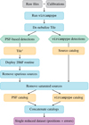 |
Fig. 2 Astrometric reduction workflow employed at the dataset level. |
3 Astrometric reduction and proper motion calculation
The data processing consisted of two workflows, shown in Figs. 2 and 3: first, each of the 11 input files was converted into a table of stellar positions and errors. Secondly, all reduced files were merged into a master catalog, and proper motions were computed.
3.1 Dataset level
The science and calibration frames for the VHS and SV tiles, respectively, were downloaded from the ESO Science Archive4. For VISIONS, we used the raw data from its second data release5.
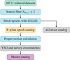 |
Fig. 3 Workflow depicting the creation of the master catalog. |
3.1.1 Reduction with vircampype
The first reduction step on the dataset level was performed with the vircampype data processing pipeline6 for VISTA data, which outperformed the Cambridge Astronomical Survey Unit (CASU) pipeline7 on VISIONS test fields (Meingast et al. 2023b). What distinguishes the vircampype procedure is that all input images are calibrated so that the epoch of source coordinates equals the observation date of an image.
The general pipeline workflow is shown in Meingast et al. (2023b), Fig. 1. In short, raw observations and calibrations are transformed into science-ready tiles and stacks, which are used to derive source catalogs containing stellar positions and magnitudes, their statistical errors, and quality flags from source extraction.
We followed the pipeline steps with two exceptions: Due to the excellent seeing conditions for most observations (Table C.1), the point sources in many datasets were close to the undersampling limit (<0.5″). Hence, we switched from a third- to a second-order Lanczos kernel for co-addition and resampling with SWarp (Bertin 2010; Gruen et al. 2014), as it performed better near the under-sampling limit on a test sample. Secondly, the extended nebulosity of the Flame Nebula was subtracted from each tile, using a custom artifact removal algorithm (Bertin et al., in prep.). The source catalog was derived from the de-nebulized image. It comprised only stars and is labeled Tile* in Fig. 2.
3.1.2 Source detection strategies
We adopted a two-pronged source detection approach using both the flux-calibrated Tiles* and their associated source catalogs from vircampype. The pipeline uses SExtractor (Bertin & Arnouts 1996) for centroid-based source extraction and aperture photometry, and calibrates the stellar positions against Gaia to ensure high accuracy. However, the central region of NGC 2024 is significantly more crowded than typical VISIONS fields, posing an edge case to the functionality of vircampype.
We found that vircampype failed to detect some sources in the dense cluster core, likely due to crowding. However, pointspread function (PSF) fitting allowed us to recover these sources, as it remains robust even in the presence of nearby or overlapping stars (e.g., Andersen et al. 2017). Using a custom IRAF/daophot pipeline, we applied PSF-fitting to the central region of each Tile*. We generated a PSF-based source list for each dataset to maximize the detection of potential cluster members. The procedure is detailed in Appendix D.
3.1.3 Saturated source removal
The saturation magnitude of the VIRCAM detectors depended on the observing conditions, selected passband, and exposure time. For the source catalog provided by vircampype, stars brighter than a limiting magnitude determined during the processing were automatically replaced with their 2MASS measurements. We removed those stars by setting the flag SURVEY==VISIONS.
For stars extracted via PSF-fitting, we manually determined the saturation magnitude for each Tile* from the radial stellar profile curves of bright stars using imexam and employed it as a filter criterion. The saturation magnitudes for each dataset, determined using both source extraction methods, are listed in Table C.2.
3.1.4 Concatenating the catalogs
On average, ~3800 sources appeared in both the vircampype catalog and the PSF-fitting source list. The former exhibited significantly higher positional accuracy when compared to the Gaia DR3 catalog for the available subset (n ~ 900, depending on the dataset). Across epochs, the standard deviation of the separation between the Gaia DR3 and the VISTA source positions ranged σα,psF ∈ [21.88,114.03] mas and σδ,PSF ∈ [20.91,110.72] mas for PSF-fitted sources, whereas vircampype positions were much better constrained, σα, vircampype ∈ [18.56,25.85] mas and σδ, vircampype ∈ [16.2,29.66] mas. Consequently, we adopted the vircampype positions for all sources present in both catalogs.
In each dataset, ~300 stars were detected exclusively with vircampype, and ~200 only via PSF-fitting (PSF-only). The former are generally faint (histogram peak at H ≈ 18.7 mag) and distributed randomly across the observed field, only sparsely populating the central region of the Flame Nebula. Their detection resulted from vircampype using a lower effective peak detection threshold than the 5σ used with daophot.
The pSF-only sources fall into two groups: (1) bright sources (H < 14 mag), likely beyond the brightness cutoff values of vircampype, that we retained with the manual cuts. They are distributed across the observed field, albeit preferentially toward the cluster center. (2) Fainter sources (H > 14) which are either close visual double stars or located in the halos of bright stars. They were likely missed in the centroid-based source extraction due to crowding or blending. Both groups contribute substantially to the cluster member census and were therefore included in the catalog, despite their lower measurement accuracy.
3.2 Master catalog level
In the second workflow (Fig. 3), the 11 processed datasets were merged into one master catalog. It comprises information on each observation, stellar positions and proper motions, auxiliary data such as YSO class, and crossmatches to other surveys.
3.2.1 Catalog cleaning and multi-epoch source matching
Having multi-epoch data available in all three passbands (pb) permitted an efficient removal of spurious detections from the source list using the source occurrence requirement Nocc, pb ≥ 2. This approach helped eliminate spurious detections, such as peaks in the variable sky background or nebulosity that were not entirely removed during de-nebulization, since these features were not detected at the exact same location in different epochs. Only two epochs were available for the J and KS filters, respectively. We used the tmatch2 function of STILTS (Taylor 2006) with a match radius of r — 0.5"to match the source coordinates between these datasets. The seven H-band epochs were cleaned using the tmatchn function and iteratively treating one epoch as a reference and identifying matches in all remaining epochs.
The purpose of the master catalog was to construct a time series of position measurements, x(t), for each star, which could be used for the proper motion calculation. All cleaned datasets were crossmatched using tmatchn (r — 0.5″), yielding the number of occurrences Nocc of each source in all datasets. Two catalogs were produced: The allstar catalog, meaning the union of all sources with Nocc ≥ 2, and the 9-plus epoch catalog containing all sources with Nocc ≥ 9. The latter was used for the proper motion calculation. The occurrence threshold was chosen as a compromise: Restricting the calculation to stars detected in all datasets (81%) would guarantee a complete sampling of the temporal baseline for each source, but ignored the fact that many likely young stars near the cluster center were detected in the H and Ks filters appear to be below the detection sensitivity in the J-band. Moreover, even with this lower threshold, the full temporal baseline was sampled for 99.89% of the sources.
 |
Fig. 4 Schematic overview of the contents of the master catalog. The full table is available online at the CDS. |
3.2.2 Proper motion calculation
Stellar proper motions along α and δ were measured using a position-error-weighted linear regression. Their uncertainties were estimated with the jackknife technique, meaning the regression model was iteratively fitted to N - 1 of the available data points N, and the slope was determined for all possible permutations. The final value of the proper motion along a given position coordinate was defined as the median of all calculated slopes. For the measurement uncertainty, we used the standard deviation estimator  , where MAD is the median absolute deviation, assuming an underlying normal distribution (Ruppert 2010). We used the standard correction
  .
.
We compared the jackknife method with classical bootstrapping and found that, while the Gaia comparisons were similarly good for both methods, the proper motion errors in both μα* and μδ from bootstrapping were substantially larger: Their standard deviations were roughly three times higher than the standard deviations for the errors estimated via jackknife, indicating that bootstrap errors were dispersed over a much broader range. While the jackknife procedure uses (N - 1)/N ∙ 100% of the data per iteration, which in our case is ≃88-99%, each bootstrap sample contains on average only ≃63.2% of the data. Because jackknife incorporates a larger fraction of the data in each iteration, it provides more stable and reliable error estimates, particularly for datasets with a limited number of observations. Therefore, using the jackknife method for the final catalog is justified.
For the vircampype catalog, where the pipeline provides correlation coefficients between the α and δ coordinates, we also tested the proper motion method intended for future VISIONS data releases (Meingast et al., in prep.). Including the coordinate correlations and fitting the full covariance matrix in the linear regression had no statistically significant impact on our calculated proper motion values (maximum deviation <0.25 mas yr−1), their uncertainties, or the results presented in Sect. 4. Since correlation coefficients are unavailable for the PSF-only sources and the results remain unaffected, we retained our original method, ensuring a homogeneous treatment of all sources.
4 The master catalog of IR proper motions
The workflows outlined in the previous section produced a master catalog of infrared proper motions for 6769 sources (Fig. 4). Of these, 194 were detected and characterized via PSF-fitting, while 6575 were taken from the vircampype source catalogs.
4.1 Core and epoch columns
The core columns of the master catalog contain the mean stellar positions, averaged over the observation epochs, the calculated proper motions, and the respective errors. For sources observed with Gaia, they also list the difference between the Gaia and infrared proper motions. The core columns further include information about the source detection method, the mean radial velocity (vLOS), if measurements were available, and various subset flags, such as YSO candidate, Gaia source, or binary candidate.
After the core columns, eleven sets of epoch columns provide information on stellar positions and magnitudes, along with their uncertainties, observation dates, and detection methodspecific details. For stars detected with vircampype, these are the exposure time, full-width half maximum (FWHM) values, and a quality flag regarding the source extraction. For sources extracted with PSF-fitting, the columns include pixel positions, their estimated errors, and the recovery fraction of cloned sources (Appendix D).
4.2 Crossmatches and YSO identification
The last part of the master catalog contains details about YSO classification, radial velocities, and photometric data from the literature. For all crossmatches, we used α and δ positions averaged over all epochs and a matching radius of r = 2″.
First, we matched the catalog with Gaia DR3, yielding 1018 total matches, 899 with 5D astrometry (α, δ, m, μα*, μδ)8. For all sources in both catalogs we calculated ∆(Gaiappm - IRppm) in the core columns. Lastly, we crossmatched with the Spitzer Legacy catalog SESNA (Gutermuth et al. 2019) to gain information in the longer wavelength ranges.
To identify young stars, we consulted the most complete YSO catalog of the region to date (Roquette et al. 2025). In particular, we used their homogeneously calculated infrared excess index αIR and their collated data on binarity, radial velocity, and possible contaminants. From the αIR classification, we identified 420 YSO candidates. After removing unclassified sources and stars flagged as main-sequence, giant, or extragalactic contaminants, we defined a bona fide sample of 362 YSOs, from Class I9 to Class III. Radial velocity information was available for 76 of these sources. When multiple measurements were present for a source, we adopted the median value and combined the associated uncertainties using inverse-variance weighting.
We investigated the 108 sources detected via PSF-fitting that were not in the YSO crossmatch. Crossmatching those sources with Spitzer and allWISE yielded 29 matches, and only two of those might be YSOs (4.5-8) μm >0.5 (Koenig & Leisawitz 2014; Spezzi et al. 2015). All other stars, only eleven of which are located in the cluster region, were not detected by those two surveys. We conclude that our YSO sample is representative and includes most young cluster members.
We also crossmatched to the photometric survey of NGC 2024 by Meyer (1996) and a disk population study based on this survey (van Terwisga et al. 2020). We discuss the YSO fraction of their surveys and the disk population of the cluster in Appendix A.
4.3 Comparison to Gaia
The proper motion histograms for all sources in the master catalog are shown in the top row of Fig. 5. The catalog includes sources with proper motions up to ±20 mas yr−1, which likely are foreground stars. Color-color and color-magnitude diagrams show that the bulk of stars in the catalog appear to be galactic background objects, with extinctions up to AV ~ 10 mag.
The bottom row of Fig. 5 shows the difference between the proper motions measured by Gaia DR3 and those determined from infrared data. The difference distributions are centered almost at zero, with very narrow FWHM values of around 1.5 mas yr−1. This indicates an excellent agreement between the Gaia and infrared measurements, with no prominent systematic offsets present for the catalog on the whole.
We note that for a shared subset between Gaia and the 98 sources determined only with PSF-fitting, we see a broader scatter of FWHM(μα*) ≈ 2.327 mas yr−1 and FWHM(μδ) ≈ 2.483 mas yr−1. The broadening is likely a direct result of the poorer positional accuracy of the PSF-fitting versus the performance of vircampype source extraction, which we observed during the direct comparison with the available Gaia data. Additionally, the median of the difference distributions in both variables is offset by about 0.2 mas yr−1. We suspect this shift originates from one or two observation epochs, where the PSF-fitting yielded the worst positional accuracy relative to Gaia (see upper limits in Sect. 3.1.4). We stress that this shift equals a velocity of 0.38 km s−1 at d ~ 400 pc, which is significantly smaller than the differences discussed later.
We examine whether the deviation between the Gaia proper motions and those derived in this work varies systematically with distance from the 2D projected cluster center in Fig. 6. Such a dependence could indicate, for instance, less accurate Gaia measurements in the cluster center due to the high optical extinction. We find no linear trend between the deviations in proper motion and radial distance. This also holds when applying different binning schemes (equal radii, equal area, or equal source number). The log-scale in Fig. 6 highlights the lack of Gaia measurements near the cluster center and the increasing source number toward the outskirts of the nebula.
In Fig. 7, we compare the measurement errors of Gaia DR3 with our results. It is evident from the significant overlap of the two distributions that the errors are on the same order of magnitude. We conclude that our proper motions are of a similar quality to the ones produced by Gaia for this region.
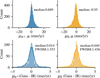 |
Fig. 5 Infrared proper motion histograms for all 6769 sources (top) and deviation from Gaia proper motions for 899 shared sources (bottom). |
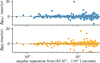 |
Fig. 6 Difference between Gaia and infrared proper motions vs. angular distance from the projected cluster center. The log-scale of the x-axis highlights the lack of Gaia sources near the center. |
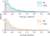 |
Fig. 7 Comparison between Gaia and IR proper motion errors. The gray shaded area indicates the overlap between the two distributions. |
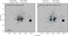 |
Fig. 8 Positions of the 362 identified bona fide YSO candidates overplotted on the inverted VHS J-band cutout. The stars are divided into still-embedded sources detected in the NIR, but not by Gaia, and optically revealed YSOs. The scale bar shows the angular scale of 1 pc at a distance of 420 pc. |
4.4 Embedded versus optically revealed YSOs
We show the positions of the YSO candidates plotted on top of an inverted VHS J-band cutout in Fig. 8. Of our 362 bona fide YSO sample, 203 appear only in our infrared catalog, which strongly suggests they are embedded sources. The other 159 stars are already optically revealed as they were detected with Gaia. This means that with our catalog, we gain proper motions for more than half (~56%) of the YSO candidates identified in the direction of NGC 2024. Moreover, the embedded population includes 58 out of 60 Class I objects, along with 89% of the Class flat YSOs, marking a > 13-fold increase in kinematic information on the youngest two YSO classes. Class II objects are almost evenly distributed between the embedded and optically revealed groups, and about 78% of Class III stars are optically revealed. The covariance matrices of the groups show that the embedded group is more centrally concentrated, with 1σ positional spreads of ~4.8′× 5.0′, compared to a larger and more elongated ~5.9′ × 7.1′for the group detected by Gaia.
5 Discussion
The positions and stellar kinematics of YSOs encode the combined influence of both their coupling to their gaseous environment and their cluster assembly history. According to recent simulations (e.g., Laverde-Villarreal et al. 2025), the way in which a cluster forms - whether through the hierarchical subcluster mergers or more monolithic growth - imprints distinct spatial and dynamical signatures on its stellar population. Similarly, the timescale over which stars decouple from their natal gas may be reflected in observed differences in the kinematic profiles of different YSO classes (e.g., Proszkow et al. 2009; Sills et al. 2018). It is worth comparing the stellar velocities to those of the surrounding gas to pin down the gas-star coupling duration. In the following, we analyze NGC 2024 concerning these questions, using the newly gained and collected information on its stellar kinematics. For this discussion, we assume that the identified YSO candidates (Roquette et al. 2025) are members of NGC 2024. We support this assumption using Fig. 8, and the calculated covariance matrices, which show that the YSO candidates - particularly the youngest - are concentrated toward the 2D projected cluster center. While some contamination cannot be ruled out, most sources are likely genuine cluster members.
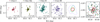 |
Fig. 9 Panels 1-4: positions of the identified YSO candidates, separated by evolutionary class. Panel 5: kernel density estimates (KDEs) at the 25% contour level. Panel 6: zoomed-in image of the cluster center. The contour linewidths decrease with increasing evolutionary stage, reflecting the YSO classes ordered by age. The scale bars are given for a distance d ~ 420 pc. |
5.1 Probing the assembly history of NGC 2024
Previous studies (Getman et al. 2014a, 2018) identified an age gradient within the central ~ 1 pc of NGC 2024, with younger sources near the cluster center and older sources toward the outskirts, based on 121 identified members. The discovery paper also lists eight scenarios for the appearance of such intra-cluster age gradients. They can be broadly grouped into:
More recent star formation in the cluster center (more dense material; accelerated star formation rate; late, central formation of massive stars and companions);
Outward movement of older stars (radial drift; dynamical heating; expansion of older subclusters);
Inward movement of young stars (late infall of filaments with already formed stars; subcluster mergers).
No scenario was favored in their study, likely in part because kinematic data for the cluster members were not previously available to evaluate the dynamical aspects of these formation pathways. As noted by Bate et al. (2003), the typical stellar velocity dispersion in young clusters (~1-5 kms−1), found in simulations and observations, allows stars to traverse distances comparable to the initial cloud radius (~0.1-0.2 pc) over typical star formation timescales of ~105 yr. Thus, positions are insufficient to evaluate cluster assembly histories.
Some formation scenarios of Getman et al. (2014a) involve subclusters, whereas others fit a more monolithic assembly. The question of monolithic versus hierarchical cluster formation is also central in simulations. They agree on an early hierarchical assembly, but diverge on how long remnants of such substructures remain observable. For instance, Laverde-Villarreal et al. (2025) reported a low-level kinematic substructure reminiscent of subcluster merger events still present after 2.5 freefall times of a cluster, even though spatial substructures have already disappeared by then. For cloud masses on the order of 104 M⊙, this would correspond to ~2.5 Myr.
In contrast, simulations by Sills et al. (2018), motivated by observed initial conditions (Getman et al. 2014b), showed a collapse of a cluster from an initially substructured state into a spherical, centrally dominated cluster already within 0.51 Myr. This collapse could also cause a variation in the velocity dispersions as a function of YSO age (Fig. 12, Sills et al. 2018).
With our homogeneous proper motion information across most YSO evolutionary classes that appear in the cluster, we revisit and discuss possible formation scenarios of NGC 2024. We do not focus on the first group of scenarios listed in Getman et al. (2014a), as they cannot be directly addressed using the kinematic information for the young stars we inferred in this study.
5.1.1 Position-age gradient and internal motion
We first investigated whether the previously reported age gradient from younger, central stars to older stars at larger radii is present in our dataset. Since we did not measure absolute stellar ages, we used YSO classes as proxies. Of the 121 sources reported in Getman et al. (2014a), 106 are included in our catalog; the 15 nonrecovered sources have 2MASS H-band magnitudes brighter than 12 mag, exceeding our saturation limit. Additionally, three sources are classified as nonmembers, and nine are flagged as main-sequence contaminants in Roquette et al. (2025).
In Fig. 9, we show the position of the cluster members divided by YSO class. Their corresponding covariance and spatial dispersion parameters are listed in Table B.1. Most Class I and flat objects are located near the central nebulosity. Class II objects occupy a larger range along the declination axis, but are still packed densely. Class III objects generally display a more scattered behavior. The covariance analysis of the YSO classes shows a clear trend from younger, more tightly clustered YSOs to older, more spatially dispersed YSOs.
The KDE is elongated in the N-S direction for the Class II and flat sources, also when considering different density thresholds. Likewise, the 1σ ellipses of Classes flat and II are elongated in the N-S direction (σδ∕σα > 1.2), while those of Class 1 stars are elongated E-W instead (σδ∕σα < 0.7). The dispersion of Class III is nearly isotropic with only a slight N-S elongation. The dominant N-S elongation of the Class II and flat-spectrum population (62% of YSOs) agrees with previous findings (Meyer et al. 2008) and suggests that stellar positions reflect the shape of the dense central nebulosity of the Flame Nebula, which itself follows the large-scale structure of the parent cloud (Hacar et al. 2024). This alignment may reflect the coupling of these YSOs to the gas, while the more evolved Class III objects are already dispersed. If the “wick” of the Flame Nebula is approximately cylindrical, the distribution of Class II and flat-spectrum sources may also trace a cylindrical three-dimensional cluster structure.
The absence of the N-S elongation trend in Class I objects could be due to their young age, extinction limiting our sample, or them experiencing different dynamical or environmental conditions than the older classes.
The spatial distribution of the different YSO classes suggests a mild age segregation between younger sources in the cluster center and older sources that populate the outskirts and parts of the center, similar to the age gradient reported by Getman et al. (2014a). While they found this gradient within the central parsec, our ~3 times bigger sample reveals differences in YSO distributions beginning within 1 pc and extending to at least 2 pc from the cluster center. However, our sample appears somewhat mixed in the cluster center, with different populations overlapping. Only in the central ~0.25 pc, seen in the right panel of Fig. 9, do we definitely see Class I objects occupying a tight space surrounded by older Class flats and a few older sources.
We transformed the proper motions into the Local Standard of Rest (LSR) and corrected them for the cluster’s bulk motion to connect the YSO positions and motions. The resulting internal kinematics of the YSO classes are displayed as vector diagrams in Fig. B.1. They show that Class I and flat sources seem to expand isotropically. Higher proper motion Class II stars show possible preferential motion along the N-S axis of the Flame Nebula’s dark lane, suggesting an influence from the gas reservoir not seen in younger populations. Class III sources show no preferred expansion trend. We observe no indications of subclusters or their remnants in our YSO sample.
We tested whether the YSOs follow a Larson-type velocity-size relation (Larson 1981; Solomon et al. 1987), but we do not find clear evidence for such a behavior in our sample (see Appendix B.3 for details). The finding is consistent with indications that the Larson relations may not hold for small spatial scales, where molecular cloud column densities can no longer be described as constant (Lombardi et al. 2010).
5.1.2 Kinematic properties across YSO classes
With the added proper motions of the optically embedded objects, we can create a more complete picture of the velocity space that the cluster occupies than previous, Gaia-based studies. Figure 10 presents 2D velocity histograms for the different YSO classes, where each source is weighted by its proper motion errors  . The weights are summed within each bin, and the binning and smoothing parameters were determined empirically to balance the resolution of velocity structures against noise from sparse sampling.
As can be seen, there is generally a large scatter of the YSO proper motions across the parameter space, regardless of evolutionary class. This finding is in agreement with previous studies. For example, Zerjal et al. (2024) identified 62 cluster members, which are difficult to discern as an overdensity in proper motion space while appearing much more concentrated in positional space. Despite containing hundreds of members, the cluster is absent from most large-scale cluster catalogs (Perren et al. 2023), likely due to the large velocity dispersion of its members and the fact that its embedded core is not detected by Gaia.
Still, the highest density peaks in the distributions of the Class flat, II, and III populations are near the mean cluster velocity marker at (0.26,-1.01) masyr−1. The same is not true for the Class I objects, where the peak is around (−0.67, −1.16) mas yr−1. The one-dimensional shift between the Class I peak and the mean cluster proper motion corresponds to ∆μα* = 0.93 mas yr−1, or around 1.85 km s−1. We note that the reported systematic shift of ca. 0.2 mas yr−1 we found between Gaia and PSF-only proper motions cannot produce this difference. It also appears when only using sources in the vircampype source catalog. However, we could not find any spatial correlation between the Class I stars producing the velocity overdensity. We also investigated the secondary peaks in the velocity distribution of Class flat and Class II, toward (−0.35, −0.35) mas yr−1, but found no spatial correlations.
To test whether the Class I proper motion is statistically different from that of the rest of the cluster, we applied meanbased permutation tests, 2D Kolmogorov-Smirnov (KS), and energy-distance tests to the (μα*, μδ) distributions of different YSO classes. The permutation test did not detect significant differences in mean velocities (p-values > 0.17). The 2D KS-test p-values were all larger than the corrected threshold of 0.05/Ntests = 0.009. The Class I versus Class III 2D KS test had the lowest value (p = 0.04). The energy-distance test, which is sensitive to differences in distribution shape as well as mean, identified only one pair (Class III vs. flat) as marginally distinct (p = 0.033), with Class III versus Class I close to the 0.05 threshold (p = 0.062). All other pairs were consistent with sharing the same distribution. Overall, we found that the kinematic distributions of YSO classes in NGC 2024 are statistically indistinguishable, even though the distribution of Fig. 10 seems to suggest substructures at first glance. The marginal difference between Class III and I/flat sources found in different statistical tests suggests that the oldest population is more dynamically dispersed than the embedded stars, but this is not a dominant effect. We conclude that all classes share a common velocity distribution within ≤2 km s−1, indicating rapid dynamical mixing or formation in a relatively coherent structure. The lack of spatial correlation for all investigated density peaks also supports this scenario.
To gain further insight into the cluster dynamics, we investigated the 1D, 2D, and 3D velocity dispersions as a function of YSO class. To determine the intrinsic velocity dispersion, we modeled the underlying velocity distribution of each YSO class. Given the limited number of observations per class, we adopted a Bayesian framework that allows for a principled treatment of uncertainty. Details about the full methodology are given in Appendix E. In brief, the velocity distribution of young stellar populations is typically well described by a multivariate normal distribution N with the covariance matrix S representing the intrinsic dispersion. Accounting for heteroscedastic Gaussian measurement uncertainties Ci of each star i, the observed velocities can be modeled as the convolution of the intrinsic multivariate normal distribution with the observational error distribution, resulting in a likelihood of the form

We used uninformative priors so that the data dominate the posterior and the inferred dispersions reflect the observed kinematics. We sampled the posterior distribution of the intrinsic 1D-3D velocity dispersions for each group using an MCMC sampler (Homan & Gelman 2014). Figure 11 shows the resulting median velocity dispersions along with their 95% credible intervals, based on 10000 posterior samples. Tangential velocities were calculated as vt(km s−1) = 4.74057 ∙ μ (mas yr−1) ∙ d (kpc), assuming d = 420 pc for stars without Gaia distances. Radial velocities are available for 76 of the 362 YSOs, resulting in smaller samples for the calculations of the two rightmost panels in the figure. Since only two radial velocity measurements are available for Class I objects, this class is excluded from the analysis of σv,LOS and σv,3D.
The velocity dispersions for Class I and Class flat range between 2.4-4.5 km s−1, overlapping but slightly higher than the 1-3 km s−1 range reported for 1-5 Myr old star-forming regions (Kuhn et al. 2019) and from simulations (e.g., Bate et al. 2003). The only deviation is the low dispersion of  kms−1. Only seven RV sources are available for this measurement, resulting in a broad credible interval that reflects its high uncertainty. The velocity dispersions of Class II are slightly higher, between 4-7.4 kms−1, while the most evolved YSOs, Class III, show considerably higher dispersions, indicating either more dynamical evolution or possible outliers in this population.
Across all velocity dimensions D, we observe the general trend of increasing velocity dispersion with evolutionary class, from Class flat to Class III. However, Class I sources depart from this trend, with velocity dispersions either equal to or exceeding those of Class flat. In 1D, Class I has a significantly higher velocity dispersion  km s−1 compared to
  km s−1, with their credible intervals directly abutting. The same trend is observed in 2D, although less pronounced. The dispersion ranges are
  km s−1 and
  km s−1, with a slight overlap of the credible intervals.
To assess the influence of potential outliers, we repeated the inference using a multivariate Student-t likelihood function with degrees of freedom ν ∈ [1,30] (see Fig. E.1). Smaller ν values correspond to heavier tails and greater robustness against outliers, while ν → ∞ recovers the Gaussian likelihood. We find that the trends of the velocity dispersions shown in Fig. 11 are preserved for all ν > D of the respective velocity variable. Further details are given in Appendix E.
This result is notable because the otherwise approximately linear increase in velocity dispersion with YSO evolutionary stage from Class flat to Class III is interrupted by the higher dispersions of Class I sources in all velocity dimensions where measurements are available. Regarding higher velocity dispersions of younger YSO classes, Sullivan et al. (2019) investigated YSO velocities in the L1688 cluster in Ophiuchus. They saw a trend for higher 1D velocity dispersion in proper motion and radial velocity for Class I/flat YSOs in the cloud core, compared to Class II/III dominated samples in the lower extinction periphery. In radial velocity, the difference between 32 embedded Class I or flat-spectrum sources was higher than that of optical surveys at the 2σ level. In our data, we only observe qualitative differences between Class I and Class flat, but we do not find the same trend they reported when comparing Class flat with Class III sources in the 2D, vLOS, and 3D velocity distributions. More radial velocity measurements for Class I objects are needed to thoroughly compare the findings in NGC 2024 to those in L1688.
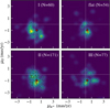 |
Fig. 10 2D proper motion histograms of the YSO classes, created with 500 bins and smoothed with a Gaussian with σ = 2 bins/pixel. The black circles show the actual proper motions, and the marker size corresponds to the weight w of a data point. The red star marks the mean YSO proper motion (0.26, −1.01) mas yr−1. |
 |
Fig. 11 Evolution of the velocity dispersions of the different YSO classes. The blue markers show the posterior median velocity dispersion alongside the 95% credible intervals. We note that insufficient Class I data are available for the two rightmost panels. |
5.1.3 Comparison of different formation theories
Connecting our analysis to the proposed star formation scenarios for NGC 2024, the findings of Sect. 5.1.1 agree with an outward drift of older stars, which can be directly seen from the stellar positions and directions of the proper motion vectors (Figs. 9 and B.1). Considering the higher 3D velocity dispersions reported for Class II and III objects, the outward movement of the older stars could be at least in part driven by N-body interactions, in accordance with simulations (Bate et al. 2003).
There is no evidence from our analysis that young stars are currently moving toward the core of NGC 2024 due to the infall of filaments with already formed stars. Furthermore, we find no statistically significant spatio-kinematic subclusters in NGC 2024. This result contradicts the suggestion of prolonged (~2 Myr) subcluster expansion or hierarchical mergers causing the age gradient (Getman et al. 2014a). It also disagrees with the simulations by Laverde-Villarreal et al. (2025) as no statistically significant kinematic imprint of subcluster mergers seems to appear in our analysis despite the young cluster age (Sect. 5.1.2).
Instead, our results align with the findings of Kuhn et al. (2019), who showed that evidence of hierarchical formation is no longer detectable in star-forming regions aged 1-5 Myr. Our analysis even strengthens their conclusion, as it also incorporates the kinematics of the embedded cluster population, whereas their study was limited to Gaia proper motions of more evolved objects. Our findings would therefore support either a relatively coherent, monolithic formation of NGC 2024, or a rapid and complete dynamical mixing of any initial substructure on timescales <1 Myr, as proposed by Sills et al. (2018) and also detailed in Kuhn et al. (2019). Their simulation matches our science case for various reasons: First, the filament structure of the Flame Nebula would be well-represented, as they modeled their initial structure as a chain of subclusters. However, the simulation is considerably more massive (3000 M⊙) than our cluster. Secondly, their simulations can produce rising velocity dispersions for younger YSOs, which also depend on the gas mass of the cluster. While our 1D and 2D velocity profiles as a function of relative YSO age differ from theirs in terms of absolute numbers, the qualitative trend of changing velocity dispersion across YSO classes is visible in our sample (e.g., Kuhn et al. 2019, Fig. 19). The rapid collapse and rebound of the cluster could account for a higher velocity dispersion of the Class I population, while remaining consistent with the finding that all proper motions originate from the same distribution. We note, however, that our Class III objects deviate from the flattened velocity dispersion trend seen in their simulations. Lastly, Sills et al. (2018) state that intra-cluster age gradients (Getman et al. 2014a) could be preserved for up to 2 Myr in their simulations, accompanied by gradual inward mixing of older stars. This agrees with the results presented in Fig. 9 and the estimated age of NGC 2024 of <2 Myr.
We note that the kinematic structure we observe in Fig. 11 could also be a projection effect arising from the viewing angle and the elongated shape of the cluster, as suggested by Proszkow et al. (2009). If it is real, however, it could indicate a super-virial state of less evolved objects in the cloud core reported by Sullivan et al. (2019). In our data, only the youngest sources (Class I) show an elevated velocity dispersion, while the Class flats produce a local minimum. This could mean that the cluster had just rebounded following its initial collapse when the youngest YSOs in our sample were formed (Kuhn et al. 2019; Sills et al. 2018).
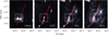 |
Fig. 12 Location of the center of NGC 2024 (white square) and the PV diagram path (red line) for Figs. 13 and 14. The panels show a cutout of the VHS Ks-band observation, and the maximum gas temperature for the (1 - 0) molecular transitions of N2H+, HNC, and HCN. |
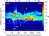 |
Fig. 13 PV diagram of 12CO(3 - 2) from the ALCOHOLS survey, with YSOs from our radial velocity sample overlaid. The gas diagram was taken from Stanke et al. (2022), Fig. 25, with the authors’ permission. |
5.2 Connection to gas velocity
To assess the star-gas coupling of NGC 2024, we compared the radial velocity subset of 76 bona fide YSOs with gas velocities of the Flame Nebula region using position-velocity (PV) diagrams along the path shown in Fig. 12. We used the gas tracers N2H+, HNC, and HCN, measured in the IRAM 30m ORION-B Large Program (Pety et al. 2017, PIs: M. Gerin and J. Pety), and 12CO(3 - 2) measurements of the ALCOHOLS survey (Stanke et al. 2022). The ORION-B data have an angular resolution of 31″ and a velocity resolution of 0.5 km s−1, while the ALCOHOLS data provide 19″ and 0.25 km s−1, respectively.
We observe a good agreement between Class I, Class flat, and most Class II and Class III sources and the 12CO gas in Fig. 13. Class III objects seem more scattered than their younger counterparts. Interestingly, some Class flat objects correlate well with high-temperature gas between 350-500″ separation, while many older sources appear in regions of lower gas temperature.
However, 12CO(3 - 2) is optically thick and predominantly traces warm gas near low-density H II regions. Therefore, we also looked at the (1 - 0) transitions of the commonly used dense gas tracers N2H+, HCN, and the more diffuse tracer HCN (Pety et al. 2017), for which the temperature can be linearly related to the gas density (Tafalla et al. 2023). As seen in Fig. 14, the agreement between stars and gas components is generally good for HNC and HCN. Class flat aligns best with regions of densest gas. While some Class II and III YSOs are already quite dispersed from the gas velocities, others still show a tight correlation in radial velocity. The two Class I objects are less in agreement with the gas velocities, but have significant error bars and low number statistics.
There is little N2H+ emission, and the gas velocity seems slightly shifted compared to the velocities of the stars. These observations agree with analyses by Hacar et al. (2024); Socci et al. (2024), who find that protostars in the Flame Nebula have a weaker positional correlation to N2H+ than other nearby regions, suggesting a rapid dispersal and photo-dissociation of dense gas by feedback from nearby massive stars like IRS 2b. As the ORION-B survey has a lower resolution than the ALCOHOLS survey, interpretations of the agreements are generally more difficult.
We find an overall good agreement between the gas and radial velocities of the young stars in our sample. While Class III and some Class II YSOs show a larger scatter, suggesting they may have started decoupling from the gas, Class flat stars clearly maintain a connection to the gas in radial velocity. We can extrapolate that if the coupling in radial velocity remains intact for those YSOs, it should also be true for the transversal (proper) motions. This means that approximating the 3D motions of the Flame Nebula using, for instance, Class II YSOs, of which many are visible in Gaia, would be a reasonable assumption and should yield good estimates. Regarding the formation scenarios discussed in Sect. 5.1.3, the good agreement between gas and stellar velocities indicates that the theorized outward motion of older stars so far seems to be a mix between radial drift and dynamical heating, with Class II and III objects likely transitioning toward the dynamical heating-dominated regime.
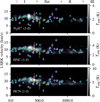 |
Fig. 14 PV diagrams of the (1 - 0) molecular transitions of N2H+, HNC, and HCN (Pety et al. 2017), overlaid with the stars in our radial velocity sample. |
6 Conclusions
In this study, we carried out the first homogeneous infrared proper motion calculation for stars in the direction of the Flame Nebula. Despite the challenge of deriving proper motions from ground-based data for sources at the cluster distance of ~420 pc in the direction of the galactic anti-center, our results are of comparable quality to the Gaia measurements for the region. This enabled us to perform the first homogeneous spatio-kinematic study of both its optically visible YSOs and the comparatively younger, still embedded stars.
We present an infrared-based proper motion catalog for 6769 stars in the direction of NGC 2024, among which we identified 362 YSO candidates. We confirmed the appearance of an age segregation and a mild gradient from young sources in the cluster center to older ones in the outskirts (Getman et al. 2014a).
Regarding the formation history of NGC 2024, our findings support an outward motion of older stars, driven partly by N-body interactions and consistent with the higher velocity dispersions of Class II and III objects, but constrained by the fact that many YSOs seem to be still kinematically coupled to their surrounding gas. We find no evidence for inward motions associated with filamentary infall or remnants of hierarchical cluster assembly. All classes statistically share a common velocity distribution, with no trace of substructure detectable to date. This observation is consistent with a formation scenario involving either the rapid collapse of a string of subclusters into a monolithic structure or formation within a relatively coherent structure. The transversal velocity dispersions of Class I YSOs are slightly higher than those of Class flat, suggesting they may have formed during the rebound phase following the initial collapse.
We report a good agreement between the gas velocity and the radial velocities of our YSO sample. Some Class II and III YSOs might be decoupling from the gas due to their larger scatter, while others retain a close connection. We extrapolate that, at least for the Flame Nebula, inferring 3D motions using proper motions of YSOs up to Class II would be justified.
With access to precise positional and velocity data of the youngest stars of a cluster, we are now at the precipice of resolving its star formation history for the first time. However, the surprising findings of a higher velocity dispersion of very young YSOs in L1688 and a hint of it in Orion highlight our knowledge gaps in the early stages of star formation. It also presents a pressing need for more radial velocity measurements of Class I objects in NGC 2024, to be able to extrapolate the tentative trend seen in the proper motion dispersion toward the third velocity dimension and assess their coupling to the gas.
Data availability
The full master catalog described in Sect. 4 will be available at the CDS via https://cdsarc.cds.unistra.fr/viz-bin/cat/J/A+A/706/A210
Acknowledgements
We thank the anonymous referee for the useful comments that helped to improve this publication. Co-Funded by the European Union (ERC, ISM-FLOW, 101055318). Views and opinions expressed are, however, those of the author(s) only and do not necessarily reflect those of the European Union or the European Research Council Executive Agency. Neither the European Union nor the granting authority can be held responsible for them. AS acknowledges funding from the European Research Council (ERC) under the European Union’s Horizon 2020 research and innovation programme (Grant agreement No. 851435). This work is based on observations collected at the European Southern Observatory under ESO programme(s) 60.A-9285, 179.A2010, and 198.C-2009. This work has made use of data from the European Space Agency (ESA) mission Gaia (https://www.cosmos.esa.int/gaia), processed by the Gaia Data Processing and Analysis Consortium (DPAC, https://www.cosmos.esa.int/web/gaia/dpac/consortium).
References
- Alves, J., Zucker, C., Goodman, A. A., et al. 2020, Nature, 578, 237 [NASA ADS] [CrossRef] [Google Scholar]
- Andersen, M., Zinnecker, H., Moneti, A., et al. 2009, ApJ, 707, 1347 [Google Scholar]
- Andersen, M., Gennaro, M., Brandner, W., et al. 2017, A&A, 602, A22 [NASA ADS] [CrossRef] [EDP Sciences] [Google Scholar]
- André, P., Men’shchikov, A., Bontemps, S., et al. 2010, A&A, 518, L102 [NASA ADS] [CrossRef] [EDP Sciences] [Google Scholar]
- Arnaboldi, M., Petr-Gotzens, M., Rejkuba, M., et al. 2010, The Messenger, 139, 6 [NASA ADS] [Google Scholar]
- Arnaboldi, M., Delmotte, N., Gadotti, D., et al. 2019, The Messenger, 178, 10 [NASA ADS] [Google Scholar]
- Arzoumanian, D., André, P., Könyves, V., et al. 2019, A&A, 621, A42 [NASA ADS] [CrossRef] [EDP Sciences] [Google Scholar]
- Bate, M. R., Bonnell, I. A., & Bromm, V. 2003, MNRAS, 339, 577 [NASA ADS] [CrossRef] [Google Scholar]
- Bertin, E. 2010, SWarp: Resampling and Co-adding FITS Images Together, Astrophysics Source Code Library [record ascl:1010.068] [Google Scholar]
- Bertin, E., & Arnouts, S. 1996, A&AS, 117, 393 [Google Scholar]
- Bolatto, A. D., Leroy, A. K., Rosolowsky, E., Walter, F., & Blitz, L. 2008, ApJ, 686, 948 [NASA ADS] [CrossRef] [Google Scholar]
- Cabezas, A., Corenflos, A., Lao, J., et al. 2024, arXiv e-prints [arXiv:2402.10797] [Google Scholar]
- Cao, Z., Jiang, B., Zhao, H., & Sun, M. 2023, ApJ, 945, 132 [NASA ADS] [CrossRef] [Google Scholar]
- Dai, Y.-Z., Liu, H.-G., Yang, J.-Y., & Zhou, J.-L. 2023, AJ, 166, 219 [Google Scholar]
- Dalton, G. B., Caldwell, M., Ward, A. K., et al. 2006, SPIE Conf. Ser., 6269, 62690X [Google Scholar]
- Emerson, J. P., Sutherland, W. J., McPherson, A. M., et al. 2004, The Messenger, 117, 27 [NASA ADS] [Google Scholar]
- Emerson, J., McPherson, A., & Sutherland, W. 2006, The Messenger, 126, 41 [NASA ADS] [Google Scholar]
- Getman, K. V., Feigelson, E. D., & Kuhn, M. A. 2014a, ApJ, 787, 109 [NASA ADS] [CrossRef] [Google Scholar]
- Getman, K. V., Feigelson, E. D., Kuhn, M. A., et al. 2014b, ApJ, 787, 108 [Google Scholar]
- Getman, K. V., Feigelson, E. D., Kuhn, M. A., et al. 2018, MNRAS, 476, 1213 [NASA ADS] [CrossRef] [Google Scholar]
- Großschedl, J. E., Alves, J., Teixeira, P. S., et al. 2019, A&A, 622, A149 [NASA ADS] [CrossRef] [EDP Sciences] [Google Scholar]
- Großschedl, J. E., Alves, J., Ratzenböck, S., et al. 2025, A&A, submitted [Google Scholar]
- Gruen, D., Seitz, S., & Bernstein, G. M. 2014, PASP, 126, 158 [CrossRef] [Google Scholar]
- Gutermuth, R., Dunham, M., & Offner, S. 2019, in American Astronomical Society Meeting Abstracts, 233, 367.10 [Google Scholar]
- Hacar, A., Alves, J., Forbrich, J., et al. 2016, A&A, 589, A80 [NASA ADS] [CrossRef] [EDP Sciences] [Google Scholar]
- Hacar, A., Socci, A., Bonanomi, F., et al. 2024, A&A, 687, A140 [NASA ADS] [CrossRef] [EDP Sciences] [Google Scholar]
- Heyer, M., Krawczyk, C., Duval, J., & Jackson, J. M. 2009, ApJ, 699, 1092 [Google Scholar]
- Homan, M. D., & Gelman, A. 2014, J. Mach. Learn. Res., 15, 1593 [Google Scholar]
- Koenig, X. P., & Leisawitz, D. T. 2014, ApJ, 791, 131 [Google Scholar]
- Könyves, V., André, P., Arzoumanian, D., et al. 2020, A&A, 635, A34 [Google Scholar]
- Kounkel, M., Hartmann, L., Loinard, L., et al. 2017a, ApJ, 834, 142 [Google Scholar]
- Kounkel, M., Hartmann, L., Mateo, M., & Bailey, III, J. I. 2017b, ApJ, 844, 138 [NASA ADS] [CrossRef] [Google Scholar]
- Kuhn, M. A., Hillenbrand, L. A., Sills, A., Feigelson, E. D., & Getman, K. V. 2019, ApJ, 870, 32 [CrossRef] [Google Scholar]
- Kumar, M. S. N., Palmeirim, P., Arzoumanian, D., & Inutsuka, S. I. 2020, A&A, 642, A87 [EDP Sciences] [Google Scholar]
- Lada, C. J., & Lada, E. A. 2003, ARA&A, 41, 57 [Google Scholar]
- Larson, R. B. 1981, MNRAS, 194, 809 [Google Scholar]
- Laverde-Villarreal, E., Sills, A., Cournoyer-Cloutier, C., & Arias Callejas, V. 2025, ApJ, 989, 22 [Google Scholar]
- Levine, J. L., Steinhauer, A., Elston, R. J., & Lada, E. A. 2006, ApJ, 646, 1215 [NASA ADS] [CrossRef] [Google Scholar]
- Lombardi, M., Alves, J., & Lada, C. J. 2010, A&A, 519, L7 [NASA ADS] [CrossRef] [EDP Sciences] [Google Scholar]
- McMahon, R. G., Banerji, M., Gonzalez, E., et al. 2013, The Messenger, 154, 35 [NASA ADS] [Google Scholar]
- Meingast, S., Alves, J., Bouy, H., et al. 2023a, A&A, 673, A58 [NASA ADS] [CrossRef] [EDP Sciences] [Google Scholar]
- Meingast, S., Bouy, H., Fürnkranz, V., et al. 2023b, A&A, 673, A59 [NASA ADS] [CrossRef] [EDP Sciences] [Google Scholar]
- Meyer, M. R. 1996, PhD thesis, Max-Planck-Institute for Astronomy, Heidelberg [Google Scholar]
- Myers, P. C. 2009, ApJ, 700, 1609 [Google Scholar]
- Meyer, M. R., Flaherty, K., Levine, J. L., et al. 2008, in Handbook of Star Forming Regions, Volume I, 4, ed. B. Reipurth (Astronomical Society of the Pacific), 662 [Google Scholar]
- Perren, G. I., Pera, M. S., Navone, H. D., & Vázquez, R. A. 2023, MNRAS, 526, 4107 [NASA ADS] [CrossRef] [Google Scholar]
- Petr-Gotzens, M., Alcalá, J. M., Briceño, C., et al. 2011, The Messenger, 145, 29 [NASA ADS] [Google Scholar]
- Pety, J., Guzmán, V. V., Orkisz, J. H., et al. 2017, A&A, 599, A98 [NASA ADS] [CrossRef] [EDP Sciences] [Google Scholar]
- Posch, L., Miret-Roig, N., Alves, J., et al. 2023, A&A, 679, L10 [NASA ADS] [CrossRef] [EDP Sciences] [Google Scholar]
- Posch, L., Alves, J., Miret-Roig, N., et al. 2025, A&A, 693, A175 [NASA ADS] [CrossRef] [EDP Sciences] [Google Scholar]
- Proszkow, E.-M., Adams, F. C., Hartmann, L. W., & Tobin, J. J. 2009, ApJ, 697, 1020 [NASA ADS] [CrossRef] [Google Scholar]
- Prusti, T., Bruijne, J. H. D., Brown, A. G., et al. 2016, A&A, 595 [Google Scholar]
- Ratzenböck, S., Großschedl, J. E., Alves, J., et al. 2023, A&A, 678, A71 [NASA ADS] [CrossRef] [EDP Sciences] [Google Scholar]
- Roquette, J., Audard, M., Hernandez, D., et al. 2025, A&A, 702, A63 [NASA ADS] [CrossRef] [EDP Sciences] [Google Scholar]
- Ruppert, D. 2010, Statistics and Data Analysis for Financial Engineering, Springer Texts in Statistics (Springer New York) [Google Scholar]
- Sills, A., Rieder, S., Scora, J., McCloskey, J., & Jaffa, S. 2018, MNRAS, 477, 1903 [Google Scholar]
- Skinner, S., Gagné, M., & Belzer, E. 2003, ApJ, 598, 375 [NASA ADS] [CrossRef] [Google Scholar]
- Socci, A., Hacar, A., Bonanomi, F., Tafalla, M., & Suri, S. 2024, A&A, 690, A376 [NASA ADS] [CrossRef] [EDP Sciences] [Google Scholar]
- Solomon, P. M., Rivolo, A. R., Barrett, J., & Yahil, A. 1987, ApJ, 319, 730 [Google Scholar]
- Spezzi, L., Petr-Gotzens, M. G., Alcalá, J. M., et al. 2015, A&A, 581, A140 [NASA ADS] [CrossRef] [EDP Sciences] [Google Scholar]
- Stanke, T., Arce, H. G., Bally, J., et al. 2022, A&A, 658, A178 [NASA ADS] [CrossRef] [EDP Sciences] [Google Scholar]
- Sullivan, T., Wilking, B. A., Greene, T. P., et al. 2019, ApJ, 158, 41 [Google Scholar]
- Swiggum, C., Alves, J., Benjamin, R., et al. 2024, Nature, 631, 49 [NASA ADS] [CrossRef] [Google Scholar]
- Tafalla, M., Usero, A., & Hacar, A. 2023, A&A, 679, A112 [NASA ADS] [CrossRef] [EDP Sciences] [Google Scholar]
- Taylor, M. B. 2006, in Astronomical Society of the Pacific Conference Series, 351, Astronomical Data Analysis Software and Systems XV, eds. C. Gabriel, C. Arviset, D. Ponz, & S. Enrique, 666 [Google Scholar]
- Vallenari, A., Brown, A. G., Prusti, T., et al. 2023, A&A, 674 [Google Scholar]
- van Terwisga, S. E., van Dishoeck, E. F., Mann, R. K., et al. 2020, A&A, 640, A27 [NASA ADS] [CrossRef] [EDP Sciences] [Google Scholar]
- Zerjal, M., Martín, E. L., & Pérez-Garrido, A. 2024, A&A, 686, A161 [NASA ADS] [CrossRef] [EDP Sciences] [Google Scholar]
- Zucker, C., Speagle, J. S., Schlafly, E. F., et al. 2019, ApJ, 879, 125 [NASA ADS] [CrossRef] [Google Scholar]
Only 808 sources have ϖ ≥ 0.
Roquette et al. (2025) do not separate Class 0 from Class I objects. Because our dataset is NIR-based and visual inspection shows no evidence for genuine Class 0 sources, we adopt their Class 0/I category as equivalent to Class I.
Appendix A Sample comparison and protostellar disk populations
One of the earliest NIR surveys on the embedded center of NGC 2024, which remains an actively used member catalog, was conducted by Meyer (1996). Their original table of observed sources encompasses 233 objects, of which 216 were measured in at least one of the JHKs passbands. No membership indicators are included in this photometric observation list. Recently, using a spatially defined subset of 179 of the initially identified sources, van Terwisga et al. (2020) observed protostellar disks in NGC 2024 with ALMA and presented evidence of two disk populations. They assumed each target was a disk-bearing source, but they only detected disks for 57 (~32%) of their targets. However, they inferred disk masses for detected disks, and mass limits using stacked observations for nondetections, and analyzed both under the assumption that all sources are disk-bearing. They presented two distinct disk populations, separated into a more eastern population with a higher detection rate of 45% and generally more massive disks, and a second smaller population of less massive disks with a detection rate of only ~15% toward the west of the nebula.
Given the continued usage of the Meyer (1996) catalog, we compared it to our observations and determine how many objects in their list are classified as YSOs in the (Roquette et al. 2025) literature catalog. Using r = 2″, we crossmatched 146 objects from the input catalog, including seven duplicated sources (seven pairs; identical or almost identical position coordinates). Of the uniquely matched sources, 89 are in the Roquette et al. (2025) catalog (78 bona fide), and 16 have Gaia measurements. Almost half of the bona fide matches (34) are Class I, followed by 22 Class flat, 19 Class II, and only three Class III (thin-disk) objects. This means that we can only assign a YSO class to about 35% of the objects of Meyer (1996) as YSOs from today’s point of view.
For 71 stars with photometric measurements, we report no crossmatch. An investigation of the available magnitude values indicated that around 50 could plausibly fall within the brightness range our study is sensitive to. A possible explanation of why they are missing in the catalog could be, for example, the characteristic variability in the brightness of young stars, which could prevent them from being detected in at least 9 of our epochs, or the positional accuracy of the Meyer (1996) measurements to within 2″.
Next, we compared our catalog to the catalog of detected and undetected disks published by van Terwisga et al. (2020): A crossmatch (r = 2″) between our catalog and theirs yielded an overlap between 69 of 122 undetected disks and 44 of 58 detected disks. It should be noted that 13 of the sources that were both detected disks and in our catalog are not marked as YSOs by (Roquette et al. 2025). This points to a possible misclassification based on the IR excess. Of the undetected disks, 24 are not classified as YSOs, but since no disks could be detected in the ALMA observations, a misclassification in their case is not as likely as for the detected disks. In total, our NIR catalog encompasses 113/180 ≈ 63% of theirs. Of the nonmatches, 16 are listed as YSO candidates in the NEMESIS catalog, but are missing from our sample.
Figure A.1 shows the positions of the crossmatched sample, color-coded and sized according to the respective disk masses, using a logarithmic scale. Circles in the left panel represent the YSOs where disks were detected with ALMA, while triangles in the right plot denote the sample where no disks were detected. This display aims to assess whether the previously described results of van Terwisga et al. (2020) of two disk populations can be reproduced using only our bona fide YSO sample.
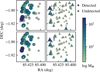 |
Fig. A.1 Positions and estimated disk masses for the subset of 144 diskbearing stars identified by (van Terwisga et al. 2020) that are also in our catalog. The sources that are not classified as YSO candidates in Roquette et al. (2025) are indicated in gray in the top row and omitted in the bottom row. The source sizes and colors correspond to their estimated masses, in units of Earth masses. The left column shows sources for which disks were detected with ALMA, while the right plot displays stars with no detected disks, where a minimum mass was derived from flux measurements. |
We concur that disk masses are generally higher toward the east of the Nebula. This is not surprising as the dense molecular ridge of the Nebula is located there (Meyer et al. 2008; van Terwisga et al. 2020). However, there are also some high mass limits for the sample of nondetections in the west, while a lot of YSOs with undetected disks and small mass limit estimates fill the space between the two extremes. We show that the previously reported mass trend also appears in our reduced sample of ~60% of the original sample size. We can not tell whether it truly indicates the presence of two distinct disk populations or simply because more dense molecular gas is available toward the east of the Flame Nebula. When only looking at the detections versus the nondetections, using the bona fide sources, we find that the median proper motion for the first group (0.39, −0.89) mas yr−1, and for the second it is slightly different, at (−0.14, −1.13) mas yr−1. A more in-depth study is needed to determine whether this shift is statistically significant and corresponds to an actual physical effect.
Appendix B Spatial dispersion, internal motion and size-velocity relation of the NGC 2024 YSOs
B.1 Spatial dispersion
Tab. B.1 lists the spatial dispersions and 95% confidence ellipse parameters for the four YSO classes shown in Fig. 9. The 1σ uncertainties in α and δ, along with their covariance, quantify the spread of each class, while the semi-major (a95) and semiminor (b95) axes describe the overall 95% confidence ellipse. Younger YSOs are more tightly clustered, whereas older YSOs show larger dispersions and more elongated distributions, indicating progressive dispersal from their birth sites consistent with cluster dynamical evolution.
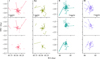 |
Fig. B.1 Position-vector diagrams of the internal motions of the NGC 2024 YSOs, divided by YSO class. For better visual differentiation, the second row shows only sources with positive motion in declination, and the third row shows stars with negative motion in declination. We note that the axis scale differs between Class I/flat and Class II/III objects. |
Spatial dispersions and 95% confidence ellipse parameters for the YSO classes. The covariance is given in arcmin2, all other values in arcmin.
B.2 Internal cluster motion
To analyze the internal cluster motions and relate them to the stellar positions, we transformed the proper motions we calculated to the Local Standard of Rest (LSR), assuming a cluster distance of d ~ 420 pc of the cluster (Zucker et al. 2019) for stars without Gaia parallax measurements. We subtracted the mean proper motion of all 362 bona fide members from each proper motion measurement. The bulk-motion corrected proper motions in the LSR are shown as vectors in Fig. B.1. The panels for Class I/flat sources are zoomed in due to the more centralized positions of those stars.
Except for Class III sources, most stars expand roughly isotropically from a central region. Class I and flat-spectrum objects show smaller proper motions than Class II sources, while Class III stars are more dispersed and no longer exhibit a clear expansion pattern. Class II sources are hard to analyze due to the crowding of many sources with small proper motions in the center. Still, the stars with larger proper motions preferentially move along the N-S axis, corresponding to the “wick” or central dark lane of the Flame Nebula. This could mean that the presence of the gas reservoir along this axis influenced the Class II motions, but the younger YSO generations no longer feel the effect.
The spatio-kinematic distribution of the YSO classes shows no clear evidence for subclusters or their remnants within our sample.
We note that three Class I stars and one flat-spectrum object exhibit unusually high proper motions for their young ages compared to the rest of their respective populations. These sources could either be runaway star candidates or contaminants in our sample. A more detailed investigation could be the subject of a future follow-up study.
B.3 Velocity-size relation
Pioneering work by Larson (1981) on the physical properties of molecular clouds showed that they obey three empirical scaling relations involving their characteristic size L (pc), mass M (M⊙), velocity dispersion σv (km s−1), and density n (cm−3):
 (B.1)
(B.1)
 (B.2)
(B.2)
 (B.3)
(B.3)
These relations were repeatedly confirmed in subsequent studies, both within the Milky Way and in external galaxies (e.g., Solomon et al. 1987; Bolatto et al. 2008; Heyer et al. 2009), although with minor variations. For instance, the exponent in Eq. (B.1), commonly denoted as α, was found to be steeper (α ≈ 0.5) in later work (Solomon et al. 1987). However, more recent studies using stars as proxies for molecular clouds in the Scorpius-Centaurus OB association reported an even steeper relation (α = 0.66) and highlight the difficulties in interpreting Eq. (B.1), given the heterogeneous methods used to derive α throughout the literature (Großschedl et al. 2025).
Because star formation is intrinsically connected to molecular clouds, and because we are studying very young objects, it is reasonable to investigate whether the scaling relations attributed to molecular clouds are also reflected in our YSO sample. Since our analysis is based on stellar astrometry, we focused on the velocity-size relation (Eq. (B.1)).
Our measurements provide only first-order approximations, as we used the two-dimensional velocity dispersion of the YSOs, σv,2D, instead of the commonly assumed three-dimensional velocity dispersion. We chose this approach because otherwise the sample would be strongly biased against the youngest objects, for which radial velocities are available only for two Class I and seven Class flat objects. Furthermore, as noted in Großschedl et al. (2025), different methods for computing the cumulative velocity dispersions and cloud sizes in the literature can affect the derived α values. As described in the main text, we computed the two-dimensional velocity dispersion as the square root of the trace of the velocity covariance matrix  . To mitigate methodological effects in the cluster size estimates, we approximated the cluster size (1) using the root-mean-square (rms) radius rrms assuming spherical geometry, and (2) using the effective radius rarea of the convex hull enclosing the stellar positions.
We grouped all YSOs into cumulative radial bins centered on the two-dimensional cluster center. We tested two definitions of the cluster center, (85.429, −1.912)10 and the mean of the YSO coordinates (85.432,-1.893), which yielded consistent results. Three binning strategies were employed: two linearly spaced schemes with 15 and seven bins, and one equal-number binning scheme with seven bins. The results are shown in Fig. B.2 for both radius calculations.
The plots show that the data do not support the expected power-law relation, as indicated by consistently low R2 values across all binning strategies. The R2 indicates how much of the variance in the data is explained by the fit, with R2 = 1 corresponding to a perfect fit. The quality of the fit degrades substantially when using more than seven bins or when adopting the equal-number binning scheme. Although the latter strategy formally yields α values in the canonical range of 0.38-0.5, these values are unreliable because the power-law fit explains little of the variance in the measured velocity dispersions. For the linearly spaced bin fits for the full range (dashed lines), the fits have higher R2 values, but the resulting α values are generally higher than the canonical range. The area-based radius estimate produces slightly lower α values than rrms, but the R2 values, i.e., the fit quality, are nearly identical between the two radius estimates.
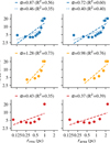 |
Fig. B.2 Two-dimensional velocity-size distributions of the YSO candidates for three binning strategies, shown with the associated powerlaw fits (dashed line). Top: 15 linear radial bins, with an additional fit to the inner 10 bins (dotted line) to test sensitivity to outer outliers; Middle: 7 linear radial bins; Bottom: 7 bins with equal star counts. |
We also considered that velocity dispersions in the outer regions could be influenced by outliers. Therefore, we repeated the fit using only the innermost 10 of the 15 linearly spaced bins (dotted line) in the top row of Fig. B.2. However, the derived α values remain unreliable because of the poor quality of the fit. Additionally, the slopes and fit quality are highly sensitive to the choice of center coordinates; however, better fits (R2 > 0.8) were only obtained for implausible center positions. Depending on the binning strategy and center coordinate choice, these fits yielded inconsistent α values, ranging from 0.5 to 1.43. Performing the same analysis per evolutionary class likewise reveals no evidence for a consistent scaling relation analogous to Eq. B.1.
We therefore conclude that our stellar sample does not follow the velocity-size relation σv ∝ Lα, with α = 0.38-0.5. The NGC 2024 cluster and the Flame Nebula are relatively small systems, and similar deviations from the classical Larson relations have already been reported on such scales. In particular, Lombardi et al. (2010) showed that Eq. B.3 does not hold for individual cores and molecular clouds because their column densities cannot be described as constant. Since n and σv are directly linked through Eqs. B.1 and B.3, a breakdown of the velocity-size relation on these small scales is therefore expected, consistent with our findings.
Observing parameters for the 11 datasets.
Appendix C Instrumentation and observing parameters
C.1 Instrumentation
All data were collected with the 4.1m Visible and Infrared Survey Telescope for Astronomy (VISTA) on the NTT peak at Cerro Paranal in Chile (Emerson et al. 2006). It hosted the VISTA InfraRed CAMera (VIRCAM) (Dalton et al. 2006), a wide-field near-infrared camera facility (0.8-2.3 μm) mounted on the telescope from 2008 until its decommissioning in early 2022. The camera consisted of a sparse 4×4 matrix of 16 detectors with a pixel size of ~0.34″. The detectors were characterized by a 1-10% deviation from linearity and saturation limit between 24,000 and 37,000 ADU (Arnaboldi et al. 2010). The camera had a seeing-limited spatial resolution, and the best achievable image quality after considering the effects of seeing, optics, and sampling was around 0.6″. Its JHKs passbands are characterized as follows: J (λc = 1.25 μm, FWHM = 0.18 μm), H (λc = 1.65 μm, FWHM = 0.3 μm), and Ks (λc = 2.15 μm, FWHM = 0.3 μm).
Further specifications of the observing instrument can be found in Emerson et al. (2004); Dalton et al. (2006); Emerson et al. (2006), on the ESO website11, or in the VIRCAM user manuals.12
C.2 Observing scheme
An observation with VIRCAM worked as follows: To create a contiguous ~1.5° × 1.0° “tile” (see Fig. 1), the smallest regular observational field, a stack of six individual images, called “pawprints”, was captured. The pawprints were taken with pre-determined offsets, ensuring that the majority of each sky position within a tile was imaged at least twice. As detailed in Emerson et al. (2004), a small, unspecified margin at the Y-axis limits of a tile remained covered only once in six pawprints. Furthermore, a pattern of smaller offsets, called jitters, was executed at each pawprint position to support the rejection of bad pixels during the co-addition process of a tile. Thus, the specific coverage of different sky positions varies across the tile (see, e.g., Meingast et al. 2023b, Fig. 4).
The typical effective exposure time across a tile is texp (s) = 2 × DIT × NDIT × NJITTER, where NDIT refers to the number of single detector integration times (DITs) that are added for one readout of the detector, and NJITTER indicates the number of jittered positions at each pawprint location.
C.3 Tables of observing parameters and saturation limits
The observing parameters for the 11 datasets used in this study are listed in Tab. C.1. The saturation limits used for source list cleaning (Fig. 2) are listed in Tab. C.2. For the PSF-fitting method, the saturation limit of each dataset was determined via imexam. For the vircampype method, they were determined during the routine (Meingast et al. 2023b).
Saturation magnitude thresholds for the 11 datasets for sources detected with vircampype (centroiding) and PSF-fitting.
Appendix D IRAF pipeline
The vircampype astrometric pipeline was specifically developed to meet the requirements of the VISIONS survey (Meingast et al. 2023b). It outperformed the CASU pipeline in various tests, but its efficiency in crowded environments, such as star clusters, which could impede the centroiding procedure used for position determinations, has not previously been tested.
To benchmark pipeline performance in these environments, we carried out an independent astrometric reduction of the Tile* images for all 11 datasets using PSF-fitting. This produced a second source catalog for each region, which we then compared to the corresponding vircampype catalog.
We used the daophot routine implemented in the large, general-purpose astronomical software Image Reduction and Analysis Facility (IRAF) Version 2.17.13 We note that this implementation is freely available as a docker image.14
D.1 Source catalog generation
The extraction of stellar positions happened in six steps, each corresponding to a daophot subroutine:
Image parameter determination - imexam
Source selection - daofind
Aperture photometry - phot
Selection of stars for PSF model - pstselect
Creation of a model PSF - psf
Positions and magnitudes for all sources - allstar
We first measured the stars’ typical full-width half-maximum (FWHM), the mean background deviation, and the minimum and maximum pixel values with imexam. Next, we performed the daofind routine with a 5σ peak detection threshold and a center box cbox = 2 × FWHM to generate a source list. We performed aperture photometry on the extracted sources using the phot routine with five different aperture sizes (1 - 5× FWHM), and sky annulus sizes according to the recommendation in the IRAF user manual for CCD photometry.15 Next, we selected candidate stars for the PSF model with the pstselect routine. This routine automatically provides the chosen number n brightest stars in the source list. However, this also includes saturated stars and is not wholly representative of the stellar content in the image. Therefore, we set n = 4000 and randomly sampled 100 sources from the provided list. We used the randomly sampled stars as input for the psf routine, adapting the PSF radius and fitting scale radius from the user manual. We inspected the surface plots of the 100 samples and retained them if the peak was well-defined and isolated, or rejected them if not. Due to the excellent seeing conditions, many observation epochs were nearly undersampled with very narrow FWHM values. Thus, we allowed for a slight asymmetry in the shapes of the peaks. A model PSF was built from fitting the retained sources, typically between 40 and 60% of the initial sample, with an analytical function. We used all five pre-defined analytical functions implemented in IRAF/daophot to generate model PSFs, which were subtracted from a given tile using the allstar command. The performance of the various models was compared based on their norm scatter values, and the best fit was used. Lastly, the subtracted image was inspected visually to determine the quality of the astrometric results.
D.2 Spurious source removal
Before running daofind, we defined a saturation threshold for each image using imexam. This ensured that the centers of the saturated sources were not in our source list, but we discovered many spurious detections appearing in their halos, likely caused by bleeding across pixels. Unlike other kinds of spurious sources, such as variations in the sky background or remnants of nebulosity, these measurements were not always removed by the filter criterion Nocc ≥ 2. To remove these misdetections, we inferred the positions of all sources brighter than the saturation limits (Tab. C.2) using the vircampype source catalog, in which bright sources are replaced with 2MASS measurements. We then empirically defined a magnitude-dependent radius around each of the 2MASS sources in our field of view brighter than 14 mag and removed multiple source detections within this area.
D.3 Positional uncertainties
The allstar routine did not provide error estimates for the extracted stellar positions, which would lead to significantly underestimated errors in proper motion for the PSF-fitted sources. So we expanded on a concept described in Andersen et al. (2009, 2017), where the authors performed completeness corrections and estimated statistical photometric errors by adding clones of their sources to their images, and re-extracting them.
Similarly, we randomly split our sample into seven subsets and added n = 100 clones of each star in a subgroup to a Tile* at random locations using addstar. The subsets ensured that we added no more than 30% of the original source list size to the image, thereby artificially inducing crowding. We then performed the daofind, phot and allstar routines again. We calculated the statistical measurement uncertainty estat from the standard deviation between input and output locations of the clones. We could also determine a recovery fraction for each star from this procedure. An example of estat,x and recovery fraction as functions of source brightness is given in Fig. D.1 for the SV H-band.
This uncertainty cannot account for all systematic effects and error contributions outside the method. However, these effects are addressed in the vircampype workflow. We added a systematic error floor esys to each statistical uncertainty to get a better overall error estimate on the positions. Its value was determined as the minimum positional errors in α and δ for each dataset using the vircampype source catalog. The final errors were computed as  . The same procedure was used to calculate the magnitude errors for PSF-only sources.
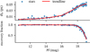 |
Fig. D.1 Statistical position error in the x pixel coordinate (top) and recovery fraction (bottom) as a function of source brightness.. |
 |
Fig. E.1 Evolution of the velocity dispersions of the different YSO classes, assuming a Student-t likelihood in the Bayesian inference model. The colored markers and shaded areas indicate the posterior median velocity dispersion, along with the 95% credible intervals for various settings of the degrees of freedom parameter ν. Insufficient Class I data are available for the two rightmost panels. |
Appendix E Bayesian inference model
We aimed to model the underlying three-dimensional velocity distribution of the stars in our bona fide YSO sample to determine the intrinsic velocity dispersion of each evolutionary class. Each class contained a limited number of stars: 54 - 171 for tangential and 2D velocities, and 7-42 for radial velocities and the full 3D velocity sample, due to the limited available radial velocities (Roquette et al. 2025). A Bayesian framework is ideal for such an analysis, as it allows for a principled treatment of uncertainty. The velocity distribution of young stellar populations can be described by a multivariate normal distribution N, with the covariance matrix S representing the intrinsic dispersion. The observed velocities can then be modeled as the convolution of this intrinsic normal distribution with the observational het-eroscedastic error distribution, meaning each source has its own measurement error Ci. The resulting likelihood can be written as vi ~ N(μ, S + Ci).
Our goal was to infer the unknown mean and covariance matrix of the error-deconvolved velocity distribution for each dimension. The posterior space included up to three dimensions from the mean and six unique dimensions from the covariance matrix. Since the covariance matrix must be symmetric and positive semi-definite, we used the Cholesky decomposition for numerical stability. By parameterizing the covariance matrix Σ via its lower triangular Cholesky matrix L, we ensured positive definiteness and allowed for correlations among the velocity components. For each dimension D = 1,..., 3, we constructed L from the parameters {lij, rij} such that Σ = LLT. This transformation mapped real-valued parameters to valid covariance and correlation structures. We used a multivariate normal distribution as our primary likelihood function, but also tested a multivariate Student-t likelihood to assess the robustness of the results against possible outliers.
We assigned Gaussian priors to the model parameters as follows: For each velocity component i = 1,...,d, the location parameters had priors μi ~ N(0,102), and the diagonal elements of the Cholesky factor were defined as lii ~ N(0,22). For dimensions D > 1, the off-diagonal correlation parameters rij (i < j) were assigned Fisher-z priors rij ~ N(0,1.52). The Fisher-z transform is a monotonic transformation that maps a correlation coefficient r, which is bounded in [−1,1], to (-∞, ∞), making inference numerically stable. The prior was defined on the transformed space, effectively covering the full back-transformed r interval.
Posterior sampling was carried out using the No-U-Turn Sampler (NUTS) (Homan & Gelman 2014) implemented in blackjax (Cabezas et al. 2024), with a warm-up phase to adapt the step size and the number of leapfrog steps. The sampler then generated 10,000 samples from the posterior distribution. For each sample, the velocity dispersion was calculated as the square root of the trace of the modeled covariance matrix. The final velocity dispersion for each parameter and YSO class was taken as the posterior median, with a 95% credible interval determined from the 2.5th and 97.5th percentiles.
The results using the multivariate normal likelihood are shown in Fig. 11 in the main text. However, due to the high velocity dispersions of Class III objects in this model, we tested the robustness of the results derived using the Gaussian model against potential outliers by also modeling the underlying velocity distribution with a multivariate Student-t likelihood. The Student-t distribution introduces an additional parameter, the degrees of freedom ν, which controls the heaviness of the distribution’s tails. As ν → ∞, it converges to a Gaussian distribution. As ν decreases, the model accommodates more points as outliers, effectively increasing the weight of central data points. We repeated the inference procedure over a range of ν ∈ [1,30] and show the results for four fixed values in Fig. E.1.
For all ν > D, where D is the dimension of the investigated velocity parameter, respectively, we qualitatively recover the same trends as for the Gaussian model. The inferred velocity dispersions become slightly smaller if more outliers are accommodated, but the overall kinematic trends remain consistent across different YSO classes and velocity parameters. In particular, Class I sources consistently have higher velocity dispersions than Class flat sources for all ν values. However, the significance of the difference between the two values decreases for smaller ν. Nevertheless, the dispersions are at least comparable, deviating from the general trend of increasing dispersion with more evolved YSO classes between Class flat and Class III. For Class II and Class III, increasing ν slightly increases the reported velocity dispersions. In 1D, the velocity dispersion of Class II is even lower than that of Class I for ν < 8 (σv,δ) and ν < 20 (σv,α*). Overall, Class I and Class II velocity dispersions are generally comparable in 1D and 2D, when the model allows for more outliers.
Because the presence of velocity outliers in the dataset is uncertain, and likely minimal for the Class I and Class flat populations, which are located in the central nebulosity of the Flame Nebula, we cannot definitely rank Class I and Class II velocity dispersions. Nevertheless, the consistency of inferred dispersion trends across the full ν range with the trends shown in Fig. 11 demonstrates that our results are robust against deviations from Gaussian velocity distributions.
All Tables
Spatial dispersions and 95% confidence ellipse parameters for the YSO classes. The covariance is given in arcmin2, all other values in arcmin.
Saturation magnitude thresholds for the 11 datasets for sources detected with vircampype (centroiding) and PSF-fitting.
All Figures
|
Fig. 1 Outlines of the SV, VHS, and VISIONS tiles covering the Flame Nebula, plotted over the Herschel Gould Belt Survey 350 μm emission map. The bold squares show the cutouts used in this study. The varying tile orientations result from the survey-specific observing strategies. |
| In the text | |
|
Fig. 2 Astrometric reduction workflow employed at the dataset level. |
| In the text | |
|
Fig. 3 Workflow depicting the creation of the master catalog. |
| In the text | |
|
Fig. 4 Schematic overview of the contents of the master catalog. The full table is available online at the CDS. |
| In the text | |
|
Fig. 5 Infrared proper motion histograms for all 6769 sources (top) and deviation from Gaia proper motions for 899 shared sources (bottom). |
| In the text | |
|
Fig. 6 Difference between Gaia and infrared proper motions vs. angular distance from the projected cluster center. The log-scale of the x-axis highlights the lack of Gaia sources near the center. |
| In the text | |
|
Fig. 7 Comparison between Gaia and IR proper motion errors. The gray shaded area indicates the overlap between the two distributions. |
| In the text | |
|
Fig. 8 Positions of the 362 identified bona fide YSO candidates overplotted on the inverted VHS J-band cutout. The stars are divided into still-embedded sources detected in the NIR, but not by Gaia, and optically revealed YSOs. The scale bar shows the angular scale of 1 pc at a distance of 420 pc. |
| In the text | |
|
Fig. 9 Panels 1-4: positions of the identified YSO candidates, separated by evolutionary class. Panel 5: kernel density estimates (KDEs) at the 25% contour level. Panel 6: zoomed-in image of the cluster center. The contour linewidths decrease with increasing evolutionary stage, reflecting the YSO classes ordered by age. The scale bars are given for a distance d ~ 420 pc. |
| In the text | |
|
Fig. 10 2D proper motion histograms of the YSO classes, created with 500 bins and smoothed with a Gaussian with σ = 2 bins/pixel. The black circles show the actual proper motions, and the marker size corresponds to the weight w of a data point. The red star marks the mean YSO proper motion (0.26, −1.01) mas yr−1. |
| In the text | |
|
Fig. 11 Evolution of the velocity dispersions of the different YSO classes. The blue markers show the posterior median velocity dispersion alongside the 95% credible intervals. We note that insufficient Class I data are available for the two rightmost panels. |
| In the text | |
|
Fig. 12 Location of the center of NGC 2024 (white square) and the PV diagram path (red line) for Figs. 13 and 14. The panels show a cutout of the VHS Ks-band observation, and the maximum gas temperature for the (1 - 0) molecular transitions of N2H+, HNC, and HCN. |
| In the text | |
|
Fig. 13 PV diagram of 12CO(3 - 2) from the ALCOHOLS survey, with YSOs from our radial velocity sample overlaid. The gas diagram was taken from Stanke et al. (2022), Fig. 25, with the authors’ permission. |
| In the text | |
|
Fig. 14 PV diagrams of the (1 - 0) molecular transitions of N2H+, HNC, and HCN (Pety et al. 2017), overlaid with the stars in our radial velocity sample. |
| In the text | |
|
Fig. A.1 Positions and estimated disk masses for the subset of 144 diskbearing stars identified by (van Terwisga et al. 2020) that are also in our catalog. The sources that are not classified as YSO candidates in Roquette et al. (2025) are indicated in gray in the top row and omitted in the bottom row. The source sizes and colors correspond to their estimated masses, in units of Earth masses. The left column shows sources for which disks were detected with ALMA, while the right plot displays stars with no detected disks, where a minimum mass was derived from flux measurements. |
| In the text | |
|
Fig. B.1 Position-vector diagrams of the internal motions of the NGC 2024 YSOs, divided by YSO class. For better visual differentiation, the second row shows only sources with positive motion in declination, and the third row shows stars with negative motion in declination. We note that the axis scale differs between Class I/flat and Class II/III objects. |
| In the text | |
|
Fig. B.2 Two-dimensional velocity-size distributions of the YSO candidates for three binning strategies, shown with the associated powerlaw fits (dashed line). Top: 15 linear radial bins, with an additional fit to the inner 10 bins (dotted line) to test sensitivity to outer outliers; Middle: 7 linear radial bins; Bottom: 7 bins with equal star counts. |
| In the text | |
|
Fig. D.1 Statistical position error in the x pixel coordinate (top) and recovery fraction (bottom) as a function of source brightness.. |
| In the text | |
|
Fig. E.1 Evolution of the velocity dispersions of the different YSO classes, assuming a Student-t likelihood in the Bayesian inference model. The colored markers and shaded areas indicate the posterior median velocity dispersion, along with the 95% credible intervals for various settings of the degrees of freedom parameter ν. Insufficient Class I data are available for the two rightmost panels. |
| In the text | |
Current usage metrics show cumulative count of Article Views (full-text article views including HTML views, PDF and ePub downloads, according to the available data) and Abstracts Views on Vision4Press platform.
Data correspond to usage on the plateform after 2015. The current usage metrics is available 48-96 hours after online publication and is updated daily on week days.
Initial download of the metrics may take a while.