| Issue |
A&A
Volume 706, February 2026
|
|
|---|---|---|
| Article Number | A177 | |
| Number of page(s) | 18 | |
| Section | Stellar structure and evolution | |
| DOI | https://doi.org/10.1051/0004-6361/202557534 | |
| Published online | 10 February 2026 | |
Mass-luminosity anomalies: Plausible evidence of recent stellar interaction in the extraordinary blue straggler S1082
1
Departamento de Astronomía, Facultad de Ciencias Físicas y Matemáticas, Universidad de Concepción 403000 Concepción, Chile
2
Department of Astrophysics, American Museum of Natural History Central Park West and 79th Street New York NY 10024, USA
3
Department of Astronomy, University of Wisconsin–Madison 475 N Charter St Madison WI 53706, USA
4
Center for Astrophysics Harvard & Smithsonian 60 Garden Street Cambridge MA 02138, USA
5
Department of Astronomy, San Diego State University San Diego CA 92182, USA
6
Department of Physics, Southern Connecticut State University New Haven CT 06515, USA
7
Adjunct Astronomer, Lowell Observatory 1400 West Mars Hill Road Flagstaff AZ 86001, USA
★ Corresponding author: This email address is being protected from spambots. You need JavaScript enabled to view it.
Received:
2
October
2025
Accepted:
10
December
2025
Abstract
Context. We present an observational and theoretical study of the complex stellar system S1082 in the open cluster M67. This system consists of at least four stars: a blue straggler in a 1.07-day eclipsing binary with a main sequence star (binary A) and another blue straggler in a 1185-day orbit with an unknown companion (binary B).
Aims. We analyzed observational data to obtain the orbital and stellar parameters of the components of the eclipsing system. We then explored mass transfer and dynamical encounter scenarios that could explain the derived properties of all of the components of S1082.
Methods. We combined high-precision photometry from K2 and TESS with archival light curves, new radial-velocity measurements, and speckle imaging to refine the orbital and physical parameters of the system. To explore the formation pathways, we conducted binary evolution simulations with MESA and dynamical scattering experiments with FEWBODY, followed by a tidal evolution modeling procedure.
Results. Our revised radial-velocity solutions yield significantly changed dynamical masses for binary A, reducing the tension with the cluster turnoff mass compared to previous studies. Speckle imaging shows two resolved components separated by 390 AU in projection and, in combination with the two spectroscopic orbits, this is suggestive of a hierarchical quadruple configuration. Our results suggest that the two blue stragglers formed separately, with later dynamical encounters assembling the present configuration. This work underscores the importance of stellar dynamics in shaping the evolution of complex stellar systems within cluster environments such as M67.
Key words: blue stragglers / stars: individual: S1082 / open clusters and associations: individual: M67
© The Authors 2026
 Open Access article, published by EDP Sciences, under the terms of the Creative Commons Attribution License (https://creativecommons.org/licenses/by/4.0), which permits unrestricted use, distribution, and reproduction in any medium, provided the original work is properly cited.
This article is published in open access under the Subscribe to Open model. This email address is being protected from spambots. You need JavaScript enabled to view it. to support open access publication.
1. Introduction
It is now widely accepted that the evolution of many Sun-like stars cannot be explained on the basis of single-star evolution alone (Mathieu & Pols 2025). Observations often show their origins to be clearly associated with evolutionary processes in binary environments. One such class is made up of blue straggler stars (BSSs), first discovered in the globular cluster M3 (Sandage 1953) and the open cluster M67 (Johnson & Sandage 1955). These are stars that have gained mass during their main sequence (MS) evolution and are still undergoing core hydrogen burning. Current theories to explain their origins focus on three plausible mechanisms: mass transfer (MT) from an evolved companion in a binary star system (McCrea 1964; Chen & Han 2008), mergers of binary stars (e.g., via angular momentum loss in stellar winds or through Kozai-Lidov oscillations in triples, Andronov et al. 2006; Perets & Fabrycky 2009), and stellar collisions during dynamical encounters (Hills & Day 1976; Portegies Zwart et al. 2010).
The old open cluster M67 (NGC 2682; 4 Gyr; Balaguer-Núñez et al. 2007) is frequently used as a canonical example of single-star evolution. However, the CMD of M67 is scattered with kinematic members of the cluster that fall in regions of the CMD that cannot be explained by single-star evolution (see Figure 1, Mathieu & Pols 2025). The BSS S1082 is particularly intriguing, as it is a remarkable multiple star system that includes two BSSs. The system exhibits complex radial-velocity (RV) and photometric variability, with the latter attributed to an eclipse as well as chromospheric activity and starspots. These features make S1082 a key object for studying binary interactions and BSS formation.
S1082 (ES Cnc, F131, MMJ 6493, WOCS2009) is a bright (V = 11.251, B − V = 0.415) star system located at α = 08:51:20.7915, δ = +11:53:26.168 (ICRS coordinates, J2000). Proper-motion studies have securely shown that S1082 is a member of M67 (Sanders 1977; Zhao et al. 1993; Geller et al. 2015b). Mathys (1991) first detected a second component in its spectrum. In the same year, Simoda (1991) reported the system to be a photometric variable. Goranskij et al. (1992) found that S1082 hosts a close binary system that has partial eclipses with a period of 1.0677978 ± 0.0000050 days. In the ROSAT study by Belloni et al. (1993), S1082 was detected as one of the brightest X-ray sources in M67. Belloni et al. (1998) suggested that this X-ray activity is generated by active regions on the surface of one of the stars in the binary system. More recently, van den Berg et al. (2004) presented Chandra observations of M67, confirming that S1082 stands out as a bright and variable X-ray source. In addition, Landsman et al. (1998) discovered an excess in the UV emission of the system, suggesting that this star is a binary with a hot subluminous companion.
van den Berg et al. (2001, hereafter, V01) presented photometric and spectroscopic data for S1082, which led them to discover a third stellar component in the spectrum. They proposed that the system is a hierarchical triple system in which two of the stars are BSSs (one in the inner eclipsing binary and the third star). According to V01, S1082 was most likely a RS Canum Venaticorum (RS CVn) system. Sandquist et al. (2003, hereafter, S03) added new photometric data and long-term RV measurements for the third star, finding it to be in an orbit with a period of 1189 days. Without conclusive evidence for a dynamical connection between the third star and the eclipsing system, these authors concluded that S1082 is either a true multiple system containing at least two BSSs or a chance superposition of two BSS cluster members, both having low, but comparable probabilities of being correct.
One particular aspect that has made S1082 a particularly notable system pertains to the masses derived by both V01 and S03 for the two stars of the inner (eclipsing) binary. According to S03, the companion star lies on the evolved MS, but has a mass of 1.6 M⊙, whereas the MS turnoff mass of M67 is 1.3 M⊙ (Geller et al. 2015a). The mass found for the primary BSS was 2.5 M⊙, but the evolutionary track passing through this star in the CMD has a mass of 1.6 M⊙ (Pols et al. 1998, see V01). This suggests that although the star is more massive than the turnoff, it appears underluminous for its inferred dynamical mass, posing a challenge for standard stellar evolution models. The radii of both stars are within their respective Roche lobes and, thus, S1082 is currently classed as a detached system (V01, S03).
Both V01 and S03 emphasized the challenge of creating the S1082 system and, in particular, the apparently subluminous stars of the inner binary system. S03 suggested that the BSS of the inner binary could have formed from mass transfer between two MS turnoff stars, although the efficiency of mass transfer would have to be very high and the remnant of the donor star would have to be exchanged out of the system. Alternatively, based on energy conservation in stellar interactions, Leigh & Sills (2011) hypothesized that the inner binary system of S1082 formed in a resonant dynamical encounter of two triples, in which multiple collisions occurred.
The system S1082 has been the subject of various recent studies. Pribulla et al. (2008) analyzed light curves (LCs) from the MOST satellite. They assumed a contact model for the LC fitting, based on the mass ratio and temperature estimates from S03. Jadhav et al. (2019) reported S1082 as a bright source in both far-ultraviolet (FUV) and X-ray wavelengths. The authors performed spectral energy distribution (SED) fitting with Kurucz models (Castelli et al. 1997), finding temperatures consistent with S03. They attributed the UV flux to stellar interactions or activity similar to the type seen in contact binaries (Jadhav et al. 2019).
The organization of this paper is as follows. In Section 2, we describe the spectroscopic, speckle, and photometric observations used in this study. Section 3 presents the analysis of the revised RV solution, speckle imaging results, LC modeling, and eclipse timing variations. In Section 4, we explore possible formation pathways for S1082 through numerical modeling, including binary evolution simulations with MESA and dynamical scattering experiments with FEWBODY followed by tidal circularization modeling. We discuss the implications of our results in Section 5, and summarize our conclusions in Section 6.
2. Observations
In this section, we describe the observational data used to characterize the system. These include space-based photometry from K2 and TESS, along with archival and newly acquired ground-based LCs, long-term RV monitoring, and high-resolution speckle imaging. Together, these observations allow us to refine the orbital solutions, determine the stellar parameters, and assess the spatial and dynamical configurations of the components.
2.1. Spectroscopic observations
The spectrum of S1082 is triple-lined, dominated by lines from a moderately rotating F star (vsini = 16 km/s). A set of 126 spectroscopic observations obtained with the former Center for Astrophysics (CfA) Digital Speedometers on both the Multiple Mirror Telescope (MMT1) and the 1.5-m Tillinghast Reflector at the Fred Lawrence Whipple Observatory (FLWO) revealed low-amplitude radial velocity (RV) variations with a period of 1185 days spanning 5.6 cycles. The RVs for this orbital solution were derived using standard correlation analysis of the Mg b region of the 126 CfA Digital Speedometer spectra reported in Table B.2, with the corresponding velocity curve plotted in Figure 3 and orbital parameters reported in Table 3.
Many of the CfA Digital Speedometer spectra also showed weak signs of very broad but shallow lines from the two stars in the one-day eclipsing binary. A TODCOR analysis yielded a marginal double-lined spectroscopic orbit for the shallow lines, but the velocity residuals were large and the results were considered unreliable, likely due to blending with the sharper lines of the primary in binary B. Thus, this orbit was not adopted for this study.
The CfA Digital Speedometers were eventually superseded by the Tillinghast Reflector Echelle Spectrograph (TRES, Szentgyorgyi & Furész 2007), a modern fiber-fed CCD spectrograph with much wider wavelength coverage and capable of spectra with much better signal-to-noise ratio (S/N). We obtained an additional 25 high-quality spectra of S1082 spanning 356 days with TRES in 2013. In the meantime Zucker, Torres, and Mazeh had extended TODCOR to handle triple-lined spectra correctly (TRICOR, Zucker et al. 1995). TRICOR models the contribution of all three stars to triple-lined spectra, thus addressing concern about distortions to the shallow RVs by the narrow-lined star. C. A. Latham carried out a preliminary analysis of the 25 new TRES spectra in 2014 using a version of TRICOR at CfA implemented by G. Torres. After some experimentation with various combinations of templates for the three stars drawn from the CfA library of calculated templates, for the best matches in the TRICOR analysis, we adopted a template with Teff = 6750 K, log g = 4.0, and v sin i = 16 km s−1 for component B; Teff = 7250 K, log g = 4.0, and v sin i = 60 km s−1 for star Aa; and Teff = 6000 K, log g = 4.0, and v sin i = 80 km s−1 for star Ab. This analysis yielded a convincing double-lined spectroscopic orbit for the eclipsing binary as shown in Figure 2, using the velocities for all three stars reported in Table B.1, with orbital parameters reported in Table 2. Interestingly, the parameters for the new orbital solution were consistent with the previous solution using the CfA Digital Speedometer TODCOR RVs.
2.2. Speckle observations
Speckle observations of S1082 were conducted using multiple high-resolution imaging instruments to resolve the individual components of the system. The Differential Speckle Survey Instrument (DSSI, Horch et al. 2009) was used at two different facilities: first on the 3.5-m WIYN2 Telescope and, later in 2016, on the 4.3-m Lowell Discovery Telescope (LDT3). In addition, observations were obtained with the NN-EXPLORE Exoplanet Stellar Speckle Imager (NESSI, Scott et al. 2018), a newer generation speckle instrument installed at the WIYN Telescope. Additional data were later collected using the Quad-camera, Wave-front-sensing, Six-wavelength-channel Speckle Interferometer (QWSSI, Clark et al. 2020) at the LDT. These instruments provided high-resolution imaging across a broad range of wavelengths, allowing for precise photometric characterization of the detected stellar components. Regardless of which telescope and instrument was used for a given observation, all data were processed as described most recently in Horch et al. (2021).
To derive the individual B and V magnitudes of the two detected sources, magnitude differences (Δm) were measured across various filters ranging from 467 nm to 880 nm. A total of 20 observations were compiled, and a best-fit linear function was applied using a least-squares minimization approach. The resulting relation between magnitude difference and wavelength allowed interpolation at the central wavelengths of the B (445 nm) and V (551 nm) filters, yielding ΔB = 0.254 ± 0.099 and ΔV = 0.286 ± 0.104. Using the known system magnitudes of S1082, B = 11.647 and V = 11.248, the individual magnitudes of the two components were determined. The primary (brighter) component was found to have BA = 12.280 ± 0.044, VA = 11.867 ± 0.045, (B − V)A = 0.413 ± 0.063. The secondary component was derived to have BB = 12.534 ± 0.055, VB = 12.153 ± 0.059, (B − V)B = 0.381 ± 0.081. The speckle measurements of the projected separation between the two resolved components are listed in Table 1.
Speckle observations of S1082 from 2012 to 2021.
2.3. Photometric observations
Time-series photometric observations of S1082 have long been challenged by the system’s orbital period of very near one day. Single ground-based telescopes, limited to nighttime observations, can only capture portions of the LC during each observing window. This introduces gaps in phase coverage and complicates the identification of eclipse features, especially in a system with such a short orbital cycle. These limitations have been significantly mitigated by recent space-based missions like Kepler/K2 and TESS (Borucki et al. 2010; Howell et al. 2014; Ricker et al. 2015), which provide nearly continuous, high-cadence monitoring over extended periods.
M67 (and S1082 specifically) were observed during Campaigns 5, 16, and 18 of the Kepler K2 mission (R. Mathieu, PI), yielding approximately 200 days of photometric data. Observations were made with a cadence of 30 minutes and an exposure time of 30 minutes, using a large 25′×25′ superstamp centered on the cluster. The LCs were extracted and corrected for K2 systematic errors using the CfA LC reduction pipeline K2SFF (Vanderburg et al. 2016). The extraction was performed using 20 apertures, and the analysis was conducted using the aperture that yielded the highest photometric precision (Vanderburg & Johnson 2014). These methods remove systematics caused by the K2 pointing drift. However, some residual long-term instrumental systematics were shown to persist and we address them later in this paper.
We also used photometric data from the Transiting Exoplanet Survey Satellite (TESS), which observes each sector of the sky continuously for ∼27 days. S1082 was observed in Sectors 44, 45, and 46 with an exposure time of 10 minutes. Light curves were produced by the MIT Quick-Look Pipeline (QLP; Kunimoto et al. 2022), which extracts photometry from full-frame images using multi-aperture photometry for sources brighter than TESS magnitude 13.5. The pipeline generates flux time series by combining data across the available observations for each target and applies standard detrending methods to mitigate instrumental systematics.
In Figure 1 we show the phased K2 and TESS LCs after applying flattening processes to the K2 data and using the orbital period P = 1.067795 days derived in our primary eclipse analysis (see Section 3.3). During the course of data exploration, we found notable variability within the K2 LCs from cycle-to-cycle. This variability manifested both in the long term (month-scale), particularly pronounced in C05, and in the short term (hour-scale), evident as dispersion in C16 and C18.
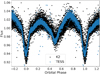 |
Fig. 1. Light curves of S1082 phased to a period of 1.067795. Black dots are K2 (K2SFF) photometry after differential photometry and flattening, while blue dots are from TESS (QLP). |
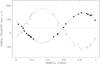 |
Fig. 2. Phased RV measurements for the eclipsing binary A, together with the RV curve for the orbital solution. Component Aa is shown as filled circles and component Ab as open circles. The orbital period used to phase the data is 1.067799 days. |
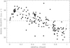 |
Fig. 3. Phased RV measurements of the binary B, together with the RV curve for the orbital solution. The orbital period used to phase the data is 1184 days. |
Therefore, to fit models to the K2 LCs with a higher level of accuracy, we applied differential photometry and flattening processes to the S1082 photometric data, enabling us to remove the long-term variability among all three campaigns. Specifically, we divided the LC of S1082 by that of the MS member S1087, which is not intrinsically variable. This star is spatially close, and lies in the same stamp as S1082. The star is sufficiently bright to minimize the contribution of photon (Poisson) noise (Howell 1989). The differential photometry effectively reduced long-term photometric shifts, most notably in Campaign 5.
However, the phased LCs continued to show low-amplitude low-frequency variation on timescales of many orbital periods across all three campaigns. Subsequent application of a flattening process successfully removed these remaining long-term trends. We performed the flattening with Lightkurve (Lightkurve Collaboration 2018), using an application called “flatten”, which removes the LC’s low-frequency trend via a polynomial fitting using scipy’s Savitzky-Golay filter (Virtanen et al. 2020). This resulted in a notable reduction in scattering within the phased LCs.
Although the flattening process alone removes most of the long-term instrumental trends in the K2 LCs, we opted to apply differential photometry using the stable cluster member S1087 prior to flattening. This step ensures the correction of low-frequency trends that might not be fully accounted for by flattening. While the LCs processed with and without differential photometry are visually similar, residual analysis reveals structured differences at the millimagnitude level, justifying the inclusion of differential photometry for maximizing precision in our final LCs.
3. Observational analysis
3.1. Orbital solution
A key result of this study is the revised RV solution for component A in S1082 (Table 2), which significantly changes the inferred stellar and orbital parameters of the system relative to previous studies. Compared to earlier analyses, particularly that of V01, which reported MAasin3i = 2.01 ± 0.38 M⊙ and MAbsin3i = 1.26 ± 0.27 M⊙, our new solution yields much lower mass estimates of MAasin3i = 1.02 ± 0.095 M⊙ and MAbsin3i = 0.774 ± 0.051 M⊙. Given the measured inclination angle of 66.7° (Section 3.3), this revision brings the mass of component Ab into closer alignment with the expected values for stars near the turnoff of M67 (MTO = 1.3 M⊙). As a result, it effectively decreases the discrepancy that had previously challenged standard evolutionary interpretations.
Spectroscopic orbit for components Aa and Ab.
The quality of the RV measurements is affected by rotational line broadening, particularly in the close binary components. Component Ab shows large velocity residuals (σAb ∼ 17 km s−1), consistent with the expectation of rapid rotation. Given the short orbital period (Porb ∼ 1.067 days), tidal synchronization is likely (Meibom & Mathieu 2005). Assuming synchronous rotation, we estimate the projected rotational velocities using
 (1)
(1)
where R is the stellar radius, P is the orbital period, and i is the orbital inclination relative to the observer. Using LC-derived radii (RAa = 1.67 R⊙, RAb = 1.77 R⊙), and adopting i = 66.7°, we find
 (2)
(2)
While no direct v sin i measurements for Aa or Ab are available, these values are significantly higher than the typical 5–9 km s−1 observed for F-type MS stars in M67 (Melo et al. 2001). The larger residuals for Ab likely reflect both its slightly higher projected rotational velocity and the increased difficulty in measuring precise RVs from broadened lines.
With a larger number of measurements, the new solution for component B also provides a more precise characterization of the orbital parameters (Table 3). The new solution is in agreement with S1082 B being part of the cluster, with a systemic velocity of γB = +33.679 ± 0.091 km s−1, consistent with the cluster mean velocity of +33.64 km s−1 (Geller et al. 2015a).
Spectroscopic orbit for narrow-line component Ba+Bb.
3.2. Speckle observations analysis
Over a nine-year observational baseline, all speckle images consistently revealed two distinct stellar sources separated by ∼0.463 arcseconds. Assuming a cluster distance of 850 pc (Geller et al. 2015a), this corresponds to a projected separation of 390 AU. No significant change in angular separation or position angle was observed during this period, suggesting negligible relative motion on the timescale of the observations.
The proper motion of S1082 is μRA = −10.1 ± 2.2 mas yr−1 and μDec = −4.2 ± 1.0 mas yr−1 (Zacharias et al. 2013). Over the nine–year span of our speckle observations, this corresponds to a displacement of roughly 90 mas in right ascension, or about twenty percent of the measured separation of the two components. Despite this, the speckle data show no significant relative motion between the two sources. This strongly suggests that A and B are co–moving at present. Two Gaia sources also are detected at approximately the same separation (∼0.43 arcsec) and position angle as the speckle measurements, although Gaia does not currently provide proper motion measurements for S1082. Future releases, particularly DR4, may provide stronger constraints.
The implications of these observations are significant. If the resolved components correspond to binary A (the close eclipsing binary) and binary B (the single-lined spectroscopic binary), then the separation and lack of relative motion are incompatible with the 1185-day orbital period inferred for component B. Assuming this separation corresponds to the semimajor axis of the wide orbit of a hypothetical quadruple system, we can estimate its orbital period using Kepler’s third law,
 (3)
(3)
where awide = 390 AU, Mbinary = 2.3 M⊙ (the mass of the close eclipsing binary), and Mwide = 1.76 M⊙ (the mass of the wide binary). Inserting these values yields

confirming a period three orders of magnitude longer than that of component B. To test whether the detected pair could be a chance alignment of unrelated stars, we estimated the probability of such a superposition within the cluster. Assuming a population of 29 BSSs in M67 (S03) distributed within a projected radius of 0.9 pc (219 arcsec), consistent with their central concentration reported by Mathieu & Latham (1986), the surface density of BSSs is approximately 1.9 × 10⁻⁴ arcsec−2. The area corresponding to a circle of 0.463 arcsec radius is ∼0.67 arcsec−2, yielding a probability of a random superposition of two BSSs of ∼1.3 × 10⁻⁴, or 0.013%. This estimate is even more conservative than the 0.4% found by S03, who used Monte Carlo simulations to evaluate BSS superpositions within 1 arcsec using the observed radial distribution of BSSs from Sandquist & Shetrone (2003), and would be lower still if using the 20 three-dimensional kinematic BSS members identified in more recent studies (Mathieu & Pols 2025).
Lastly, we computed the tidal-to-orbital acceleration ratio to evaluate the potential dynamical influence of the wide binary B on the close binary A. The result, atidal/aorbital ≈ 1.03 × 10⁻¹³, confirms that tidal effects from B are negligible. Even presuming binaries A and B are physically bound, they evolve independently on very different timescales.
Taken together, the close physical separation observed in speckle imaging and the low probability of a chance superposition, both strongly suggest that S1082 A and B are a physically associated pair of binaries in a long-period orbit (see Figure A.1 for a schematic representation). If this interpretation is correct, the projected 390 AU separation would correspond to a wide orbital period of nearly 3800 years, making the system a likely hierarchical quadruple composed of S1082 A (the eclipsing binary) and S1082 B (a single-lined spectroscopic binary). While secure proof of physical association is not yet possible, the likelihood is sufficiently high to motivate treating S1082 as a probable quadruple in the dynamical interaction models explored in Section 4.2.1.
3.3. Light-curve fitting
Considering that the timescale for variations in the shape of the LC is short (even hours), spot activity is very likely (S03). There are different methods to derive binary parameters for systems such as RS CVn stars (e.g., Budding & Zeilik 1987). The technique used here was similar to that in Pribulla et al. (2008) and S03, where pristine segments were sought.
The description of a pristine segment in this work is a segment with good phase coverage, an equal maximum brightness in the quadratures, an ellipsoidal variation, triangular-shaped eclipses, and a brighter mean flux compared to other segments (indicating a time when the surface brightness was least affected by cool starspots, which typically lower the observed flux). A segment with these characteristics should describe a time that minimizes the effects of spots on the structure of the LC. We note that we did not use TESS LCs to obtain a LC solution because all of the LCs showed clear differences between the two quadrature brightnesses. The three K2SFF campaigns containing S1082 observations were split into segments of ∼10 days duration to seek pristine segments. After a by-eye inspection, we selected one segment within K2 observations (see Figure 4). This segment had the lowest dispersion and the clearest structure, fulfilling the conditions mentioned above. However, it had a dimmer mean flux during the second quadrature. There are still asymmetries, which unavoidably requires spot modeling.
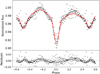 |
Fig. 4. Chosen “best segment” of the K2 C16 LC (black dots) and the best fit model (red line). The bottom panel shows the residuals from the fit. The orbital period used to phase the data is 1.067799 days. |
To obtain a LC solution, we performed the LC fitting analysis of the S1082 system using the Eclipsing Binary Learning and Interactive System (ELISa; Čokina et al. (2021)) software. Out-of-eclipse variations were modeled in ELISa using Roche geometry to account for tidal distortions, together with reflection effects from mutual irradiation and optional Doppler beaming terms, ensuring that ellipsoidal variability is reproduced consistently with the system’s geometry. ELISa initializes the modeling process with user-provided parameters and uses a non-linear large-scale least-square trust region reflective (LSTRR) algorithm implemented in SciPy (Virtanen et al. 2020), which allows a quick search for local minima within a predefined search box using a gradient method to fit the photometric data. Following this, it employs the Markov chain Monte Carlo (MCMC) technique from the emcee package (Foreman-Mackey et al. 2013) to explore the parameter space around the preliminary solution, refining the parameter estimates and producing posterior distributions along with corner plots for detailed analysis.
We used as priors the mass ratio, eccentricity, and a sin i derived in the RV solution. In the initial LSTRR stage, the mass ratio was allowed to vary uniformly within q = 0.759 ± 0.032, and the eccentricity within e = 0.019 ± 0.015. After convergence, q and e were fixed at their best-fit values for the MCMC exploration. The total projected semimajor axis from the RV fit was kept fixed throughout, implemented in ELISa by constraining a through the inclination (a = 5.34/sin i), so that a varied only in response to changes in i during the fit. The effective temperature of star Aa was initially set to 7325 K (as in S03) and then allowed to vary along with the other free parameters. The temperature ratio TAb/TAa = 0.822 ± 0.031 is more tightly constrained in the fit than the individual temperatures, consistent with expectations for eclipsing binaries. To account for the difference in brightness between the quadratures following the primary eclipse, we included a single cool spot as a free parameter (found to be at longitude = 260°, latitude = 328°, angular radius = 20.6°, temperature factor = 0.8) in the model. Comparable fits could be obtained with the spot placed in other locations. However, with only one spot in the model, the fit does not reproduce all quadrature structures. Figure 4 shows the phase-folded LC overlaid with the synthetic model.
Table 4 shows the derived parameters from the LC solution for binary A. A significant third light contribution (l3 = 0.62) was identified, consistent with their relative fluxes. To determine the positions of the stars on the CMD (Figure 5), we used the effective temperatures and bolometric luminosities derived from the LC solution. ELISa computes the Teff of each component either by fitting it directly as a free parameter (as in this case) or by fixing it based on external constraints, while the Lbol is computed assuming blackbody radiation using the Stefan–Boltzmann law. The equivalent radius is obtained numerically from the stellar surface geometry defined by the Roche potential. We converted the ELISa-derived Teff and Lbol values into Johnson–Cousins B − V colors and V magnitudes using the bolometric corrections and color–temperature relations in Table 3 of Flower (1996).
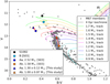 |
Fig. 5. CMD of M67 showing the positions of the components of S1082. Gray points are confirmed cluster members from Geller et al. (2015b). A 4.0 Gyr MIST isochrone (dashed black line; 850 pc, AV = 0.093, solar metallicity) and single–star evolutionary tracks from 0.9–1.7 M⊙ are overplotted. Circles mark the component positions from Sandquist et al. (2003), while triangles show the updated values derived in this study (blue: Aa, 1.30 ± 0.13 M⊙, orange: Ab, 1.00 ± 0.07 M⊙). Red arrows mark the shifts from the earlier estimates to the new ones. |
Light curve solution for the close binary A. *= from Geller et al. (2015a).
The new CMD positions highlight important deviations from single-star evolution. Notably, component Ab appears more evolved than expected for its ∼1 M⊙ mass at the age of M67. Its radius and luminosity are consistent with an evolving MS star nearing the end of hydrogen burning. Conversely, Aa’s location supports the interpretation of it being a rejuvenated BSS that has not yet begun post-MS expansion. These CMD placements reinforce the distinct evolutionary histories of the two stars and frame the broader dynamical and evolutionary context explored in the Discussion section 5.
With the discovery of component B in the composite light coming from S1082 (V01), the degree of multiplicity of S1082 has been frequently discussed (V01, S03, Leigh & Sills (2011)). A hierarchical triple configuration involving the close binary A and component B could not be confirmed in previous studies. Pribulla et al. (2008) found a high scatter in the photometric O − C diagram, where the deviations were attributed to light-time effects (LITE) caused by component B. However, the derived orbital period did not fit the observed period of the component B orbit, so the results were not conclusive.
Here we present a new analysis of the period variation, together with an updated O − C diagram (Figure 6) to search for any LITE caused by higher-order multiplicity. (With speckle data we discarded the hypothesis that component B was part of a triple system with A; see Section 3.2). We compiled primary eclipse timings from archival and modern observations, including unpublished Mount Laguna Observatory data, and new timings from K2 and TESS LCs. We segmented the photometric observations into intervals spanning single orbital cycles. Further filtering was applied to remove cycles that lacked a clearly defined primary eclipse. We did not consider the secondary eclipse, as its shape was more significantly affected by spot activity. The times of primary minimum were determined by following the method described by Deeg (2020) that returns eclipse mid (minimum)-time using the Kwee & van Woerden (1956) method with revised timing error. Using these timings, we performed a χ2 minimization over a range of trial orbital periods to identify the best-fit photometric period,
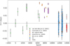 |
Fig. 6. O − C diagram of the times of the primary eclipse minima for S1082. We consider the same T0 as van den Berg et al. (2001), i.e., 2444643.25 HJD time. |

The difference between the RV and photometric period determinations is well within their measurement uncertainties.
To quantitatively assess the deviations in eclipse timings among the different observational datasets, we calculated the mean O − C residual and its associated uncertainty for each dataset, including K2, TESS, and five literature sources. Table 5 summarizes the mean residuals, root-mean-square (RMS) scatter, and standard error on the mean, defined as  where N is the number of primary minima measured in each dataset. We consider a dataset to show a statistically significant deviation in eclipse timing if the absolute value of its mean O − C residual exceeds 3σmean. Based on this criterion, the eclipse timings reported by Csizmadia et al. (2002), Mt. Laguna data, and Pribulla et al. (2008) all show statistically significant positive residuals. These measurements suggest that the primary eclipses in those epochs occurred earlier than expected under the best-fit linear ephemeris. In contrast, the TESS dataset shows a statistically significant negative residual (∼15σ), suggesting that eclipse timings occur earlier than predicted by the linear ephemeris. The K2 dataset is consistent with zero within 3σ, indicating no significant deviation from the timing model.
Statistics of O − C residuals by dataset.
The LC of S1082 is characterized by relatively shallow eclipses and a prominent, variable O’Connell effect. The high scatter present in the O − C diagram reflects the complicated determination of precise time minima in such a complex LC. While these deviations could suggest a dynamical origin such as a LITE from a third companion, we show in Section 5.2 that such an interpretation is inconsistent with independent constraints from RV and speckle observations. The true origin of the period modulation remains uncertain and likely involves complex stellar processes, which are further explored in the discussion in Sect. 5.
4. Numerical modeling
4.1. MESA mass transfer simulations
We performed simulations to test stable Case A mass transfer as the formation mechanism of binary A. We employed the stellar evolution code Modules for Experiments in Stellar Astrophysics (MESA; Paxton et al. 2011, 2013, 2015, 2018, 2019; Jermyn et al. 2023) to model a grid of binary evolution tracks. All simulations assumed conservative mass transfer, solar metallicity (Z = 0.02) and neglected stellar winds. The total progenitor binary mass was fixed at 2.3 M⊙ to reflect the observed mass of S1082 A. We explored a wide range of initial donor masses (M1,init = 1.15–1.60 M⊙ in steps of 0.01 M⊙), with the secondary mass adjusted to maintain the total mass. Initial orbital periods ranged from 0.5 to 1.1 days in 0.1-day steps.
Each model was categorized according to its evolutionary outcome. In some cases, the donor star evolved off the MS without filling its Roche lobe, thereby failing to trigger mass transfer. In others, mass transfer initiated but quickly led to a contact binary configuration in which the accretor also overfilled its Roche lobe. In our MESA framework, such configurations terminate the calculation. While our treatment treats contact as an endpoint, in reality some contact binaries may return to detached or semi-detached configurations once the accretor regains thermal equilibrium and contracts (Henneco et al. 2024), so our models may underrepresent certain possible evolutionary pathways. Here we focus on the remaining subset of models that experienced two episodes of mass transfer: the first while the donor was on the MS, and the second after core hydrogen exhaustion. We searched for configurations in which the initial mass transfer episode occurred within the first 4 Gyr, consistent with the age of M67.
After modeling 624 binary configurations, none reproduced the present-day configuration of S1082 A. The primary inconsistency lies in the evolutionary state of the current secondary star, which appears on the slightly evolved portion of the MS in the CMD, consistent with ongoing hydrogen burning and moderate helium enrichment. In contrast, all models predict that the post-mass-transfer donor would be a thermally contracting proto-white dwarf, significantly underluminous relative to the current position of star Ab in the CMD (e.g., Figure 7).
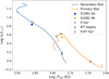 |
Fig. 7. HR diagram showing the evolution of a representative conservative MESA mass transfer model, with initial masses of 1.23 M⊙ (donor, orange) and 1.07 M⊙ (accretor, blue), and initial orbital period of 0.95 days. Filled squares mark the observed positions of S1082 Aa and Ab. Circles show the model positions at 4 Gyr, crosses indicate when mass transfer begins, and diamonds mark the positions at 4.87 Gyr after mass transfer has altered both stars’ evolution. |
This discrepancy arises because stable mass transfer strips the donor’s hydrogen-rich envelope, halting core hydrogen fusion. The resulting remnant cools and fades, becoming progressively redder. Such behavior is a well-established outcome of standard binary evolution theory (e.g., Nelson & Eggleton 2001; Lu et al. 2010). Even when mass transfer begins relatively early on the MS, our models tend to either strip too much mass (ceasing H-burning entirely) or evolve toward contact, neither of which match the observed state. Producing a ∼1.0 M⊙ MS secondary while halting mass transfer during the later stages of H burning remains an unsolved problem in our models.
A representative example from our grid of conservative mass transfer models, with an initial primary of 1.23 M⊙, a secondary of 1.07 M⊙, and an initial period of 0.95 days, illustrates the general behavior (see Figure 7). The first episode of mass transfer occurs after 4 Gyr, so at this age both components remain on their detached evolutionary tracks. At 4 Gyr, the donor (orange track) remains on the subgiant branch and happens to lie near the CMD position of S1082 Ab, but this is pre–mass-transfer. By 4.87 Gyr (marked with diamond symbols), mass transfer has occurred, the donor has left the subgiant branch and evolved toward lower luminosity, while the accretor (blue track) has gained mass and migrated toward the blue straggler region, near the current position of S1082 Aa. However, the donor’s post-transfer position is far too faint to match Ab. More generally, in our models the donor either evolves off the MS as MT begins, or evolves to the subgiant branch before starting mass transfer, moving even further away from the MS. At the same time, the accretor tends to become too massive, often exceeding 1.6 M⊙, which is inconsistent with the revised dynamical mass.
These findings hold even when relaxing constraints on the present-day dynamical masses and instead focusing solely on matching the CMD positions of the two stars. No combination of binary parameters tested could simultaneously reproduce the observed luminosity and temperature of both components at 4 Gyr. In particular, the position of the current secondary (Ab) in the CMD is incompatible with that of a post–mass-transfer remnant. In every simulation, the donor ends as a stripped, underluminous object, whereas Ab appears consistent with a MS star.
This discrepancy leaves two broad possibilities: either an atypical form of mass transfer, potentially episodic, prematurely truncated, or occurring under conditions that avoid extreme mass-ratio reversal, or the current secondary is a MS star that was dynamically inserted into the system after the original donor was lost. The latter explanation is supported by our dynamical simulations (Section 4.2), which show that BSS binaries like S1082 A can plausibly result from a combination of mass transfer and subsequent dynamical exchanges, with the present secondary replacing the original donor.
4.2. Numerical scattering simulations and tidal circularization
To explore the possibility that S1082 A formed as a result of a dynamical interaction, we performed numerical scattering simulations using FEWBODY (Fregeau et al. 2004), a toolkit designed for simulating gravitational encounters involving small-N stellar systems. While the previous section demonstrated that isolated binary evolution fails to explain the observed configuration of S1082 A, dynamical processes in a dense cluster like M67 could provide an alternative formation pathway and significantly change the picture. We modeled two different types of stellar encounters that could plausibly produce the observed system: binary-triple (2+3) and binary-single (2+1) interactions.
4.2.1. Binary-triple (2+3) interactions
As mentioned in Section 3.2, the speckle imaging analysis supports the interpretation of S1082 as a hierarchical quadruple system composed of a close binary (S1082 A) and a wider binary (S1082 B). Under this assumption, we first evaluated the energetic plausibility of this configuration. We estimated the orbital binding energy of the proposed quadruple system by treating S1082 A and B as two bound subsystems orbiting a common center of mass. The computed energy, Eorb ≈ 9.15 × 1036 J, significantly exceeds the average kinetic energy of stars in M67 (Ekin ≈ 3.46 × 1035 J), suggesting the system is dynamically “hard” and stable against disruption. With a projected separation of 390 AU this corresponds to a semimajor axis of ∼0.0019 pc, while typical inter-particle distances in M67’s core are ∼0.2 pc. This implies that a stable quadruple configuration with this separation is dynamically plausible in the cluster.
Triple star systems are now recognized as dynamically important components in star cluster environments, with interactions involving triples occurring as frequently as, or even more frequently than, those involving binaries or single stars, particularly in low-mass clusters like M67 (Leigh & Geller 2013). Higher-order multiples enhance the cross-section for dynamical encounters, increasing the likelihood of complex outcomes such as collisions or the formation of binaries (Leigh & Geller 2012). The relevance of 2+3 encounters in M67 is supported by encounter timescale estimates. Using the formalism in Appendix A of Leigh & Sills (2011), and assuming a binary fraction of 0.5 (Fan et al. 1996) and a fb/ft = 0.1 (Leigh & Sills 2011), we find that such interactions occur on timescales of ∼2 × 10⁷ years, which is much shorter than the cluster age, and well within the typical BSS lifetime (Tian et al. 2006).
Motivated by these results, we simulated 80 000 binary-triple encounters. In this setup, illustrated in Figure A.2, the incoming binary, designated as object 1, contained a BSS (1.3 M⊙, 1.67 R⊙) and a white dwarf (0.36 M⊙, 0.05 R⊙) formed through a previous episode of Case B mass transfer (Paczyński 1971). The more massive star represents the BSS in S1082 A. The WD star represents a WD remnant of an earlier episode of stable mass transfer. We focus on Case B specifically because it typically leads to stable mass transfer (Soberman et al. 1997; Ge et al. 2020; Temmink et al. 2023), which avoids the complexities and uncertainties associated with common-envelope evolution. Moreover, such stable interactions generally produce binaries with wider separations (e.g., Soberman et al. 1997), increasing the cross-section for subsequent dynamical encounters. This makes them more likely to participate in interactions like the one modeled here. The target hierarchical triple, designated as object 0, was composed of a BSS (1.4 M⊙, 1.8 R⊙) and a WD (0.35 M⊙, 0.05 R⊙) in a 3 AU, e = 0.6 inner binary (representing the BSS and its subluminous companion in S1082 B), with a 1.0 M⊙ MS star (1.77 R⊙) in a 390 AU, e = 0.3 outer orbit. The radius of the MS star in these models resembles the radius of the MS star in S1082 A. These configurations satisfy the dynamical stability criterion of Mardling & Aarseth (2001). The initial eccentricity of the incoming binary was set to zero.
In these simulations, the stellar masses and radii were fixed for all runs. The masses of the WDs were selected to allow tracking of the components post-encounter. All mass transfer events and internal stellar evolution were assumed to occur before the encounter, and thus stellar properties remained constant during the simulations. Mergers were included as possible outcomes in all runs, following FEWBODY’s “sticky star” prescription (Fregeau et al. 2004). In this approach, stars are treated as rigid spheres with radii equal to their stellar radii, merging upon contact with no mass loss and conserving linear momentum. For MS-MS collisions, the expansion factor fexp is set to 1, so the merger radius is simply Rmerger = R1 + R2. While mergers were not the primary focus of this work, they were naturally recorded in the simulation outcomes.
We varied the initial semimajor axis of the incoming binary (a1), sampling values uniformly between 0.05 AU and 4.0 AU in steps of 0.05 AU. The other orbital elements were kept fixed across all simulations. Each combination of orbital parameters defined a set of 1000 realizations (also called seeds) where the impact parameter was uniformly sampled between 0 and bmax = 5 × (a0 + a1), in units of a0 + a1, where bmax was chosen according to Fregeau et al. (2004). The velocity at infinity v∞ was drawn from a Maxwellian distribution with a velocity dispersion of 0.59 km s−1, consistent with M67’s internal kinematics (Geller et al. 2015a).
We searched specifically for outcomes matching the hierarchical structure [[0 1] [2 3]] 4 (see Figure A.2), corresponding to a hierarchical quadruple system composed of two post-encounter binaries ([0,1] and [2,3]) and a single star ejected from the system (star 4). In this nomenclature, stars 0 and 1, with masses of 1.4 and 0.35 M⊙ are the components analogous to the BSS and presumed WD in S1082 B, while stars 2 and 3 (1.0 M⊙ and 1.3 M⊙) represents the MS and BSS in S1082 A.
Among the 80 000 simulations, 227 ended in this desired configuration, corresponding to a success rate of ∼0.28%. For each successful outcome, we extracted the final orbital elements of the post-encounter (2,3) binary and the outer orbit between the two binaries.
The distribution of final orbital periods for the (2,3) binaries showed a clear dependence on the initial semimajor axis of the incoming binary. As shown in Figure 8, a sublinear power-law relation,  , was observed, indicating that tighter binaries tend to produce shorter-period remnants. Finally, close binaries with orbital periods near the observed 1.068-day period of S1082 A were produced.
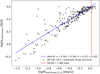 |
Fig. 8. Relation between the final orbital period of the close binary ([2 3]) and the initial semimajor axis of the incoming binary (a1) in 2+3 encounters that resulted in a quadruple-single configuration. The best-fitting linear relation is shown in blue. The red vertical line marks the location of the observed orbital period of the close binary in S1082 (1.068 days). |
However, the orbital periods between the two binaries (the full quadruple) were consistently in the 500–5000 day range, peaking around 103 days (see Figure 9). This is more than two orders of magnitude shorter than the orbital period corresponding to the observed 390 AU separation (∼106 days), and thus inconsistent with the real system. Moreover, we estimated the typical interaction timescale for such a wide quadruple system in M67 to be only 7.5 × 10⁶ years, suggesting that even if such systems form, they are unlikely to survive over Gyr timescales. These findings imply that while our 2+3 encounters can create systems with the internal architecture of S1082, they cannot simultaneously reproduce its wide separation.
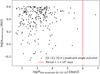 |
Fig. 9. Relation between the final orbital period of the outer quadruple system ([[0 1][2 3]]) and the initial semimajor axis of the incoming binary (a1)in 2+3 encounters that resulted in a quadruple-single configuration. The red vertical line indicates a period of 1 × 10⁶ days, which is close to the orbital timescale inferred from the projected separation of the resolved components of S1082 (390 AU). |
4.2.2. Binary-single (2+1) interactions
We next considered an alternative scenario in which S1082 A formed through a binary-single (2+1) encounter, with the assumption that the close binary S1082 A is an isolated system. In this setup, illustrated in Figure A.3, a close binary containing a BSS and a WD (again formed through earlier Case B mass transfer) interacts with a single 1.0 M⊙ MS star. If the WD is ejected and the MS star captured, this can yield a BSS–MS binary without requiring a subsequent mass transfer phase.
To explore this possibility, we performed 59 independent FEWBODY simulations of 1 000 seeds each, for a total of 59 000 2+1 encounters. The initial binary consisted of a BSS (1.3 M⊙, 1.67 R⊙) and a WD (0.36 M⊙, 0.01 R⊙). The incoming single was a 1.0 M⊙ MS star. As in the 2+3 simulations, the impact parameter b and the velocity at infinity v∞ were drawn from a uniform distribution and a Maxwellian distribution corresponding to the kinematic environment of M67, respectively. All runs used fixed stellar masses and radii, and assumed circular orbits, as perhaps are created during the earlier mass transfer. Mergers were also tracked in these runs using the same FEWBODY prescription, with fexp = 1. The initial semimajor axis of the binary (A1) was varied from 0.05 to 3.0 AU in steps of 0.05 AU. This design allowed us to systematically probe the sensitivity of the encounter outcomes to the initial binary separation.
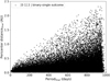 |
Fig. 10. Distribution of the final orbital periods and pericenter distances for all FEWBODY simulations that produced the desired [0 1] 2 binary-single outcome. |
Each set yielded a dominant number of binary-single outcomes ([0 1] 2), with 38 032 (64.46%) producing this configuration. This outcome corresponded to a BSS-MS binary system and a single WD (see Figure A.3). The distribution of the final orbital periods and pericenter distances of the simulations that ended in the wanted outcome is shown in Figure 10. We found that for small values of A1 (< 0.1 AU), the simulations were strongly dominated by merger events, with very few binary-single outcomes. However, for A1 values above 1 AU, the desired outcome stabilized at ∼70% frequency across seeds. Among these binaries, 737 had orbital periods < 100 days and 173 had pericenter distances < 0.05 AU, close to the semimajor axis of S1082 A (∼0.02 AU), representing a fraction of ∼0.3% of the total simulations. Furthermore, only four systems achieved orbital periods < 10 days, with the shortest at 5.67 days. Thus, while the pericenter distances became compact, the orbital periods remained significantly longer than the observed value.
4.2.3. Tidal circularization with MESA
Given the pericenter compactness of several binaries formed in 2+1 interactions, we explored whether tidal circularization could reduce their periods to match S1082 A. To do this, we selected nine post-encounter binaries with final periods < 100 days (blue crosses at Figure 11) and evolved them using MESA, incorporating tidal synchronization and circularization.
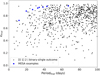 |
Fig. 11. Final orbital eccentricity vs. period for all FEWBODY simulations that produced the desired [0 1] 2 binary-single outcome with Pfinal < 100 days. Blue crosses show the subset of systems selected for MESA tidal circularization modeling. |
Initial orbital parameters from FEWBODY simulations used as input for MESA tidal circularization models, and the resulting final orbital period at 4 Gyr.
Each system was initialized using the final orbital period (Pinitial) and eccentricity (einitial) from FEWBODY. The primary was modeled as a 1.3 M⊙ star, and the secondary as a 1.2 M⊙ star, higher than the observed 1.0 M⊙ value for Ab, to reflect its anomalously large radius (∼1.77 R⊙), which would enhance tidal effects. The systems were evolved to 4 Gyr.
Final periods ranged from 1.215 to 3.76 days (see Table 6), with the shortest (Run 38) approaching the observed 1.068-day period of S1082 A. Several runs ended with final periods within 15% of the observed value. These results represent more than an order-of-magnitude orbital decay from the original periods (11–67 days), highlighting the efficiency of tidal circularization. The distribution of eccentricity versus final period is shown in Figure 11, and the initial and final periods are listed in Table 6.
While none of the runs reproduced S1082 A’s period, they show that tidal circularization following a 2+1 interaction is a viable mechanism for producing close, detached BSS–MS binaries. Modest changes in initial conditions, like slightly shorter separations or more extreme eccentricities, could plausibly yield the observed period, especially when accounting for uncertainties in tidal dissipation physics. Furthermore, MESA models treat the BSS as a canonical MS star, neglecting potentially critical structural peculiarities that would affect tidal evolution. Similarly, the larger-than-expected radius of the secondary implies unusually deep convection, potentially enhancing tidal dissipation.
Thus, although our present simulations fall slightly short of the precise configuration of S1082 A, they support a two-step formation pathway: BSS formation via mass transfer, followed by a dynamical exchange and tidal circularization, potentially involving enhanced structural dissipation mechanisms not yet implemented in current models.
5. Discussion
This section discusses the main findings derived from the observational analysis and theoretical modeling of S1082. We first examine the consistency of the stellar and orbital parameters derived from the RV and LC solutions. We then investigate potential sources of variability in the eclipse timing diagram. Lastly, we evaluate the implications of our FEWBODY and MESA simulations for the formation of the system and consider whether the observed configuration is more consistent with isolated or coupled dynamical origins for the two subsystems.
5.1. Stellar and orbital parameters
The RV and LC solutions for the binary A in S1082 confirm several key features of the system’s geometry and stellar properties, while also raising notable questions regarding the internal structure and evolutionary state of its components. Compared to earlier work, particularly the solution from V01, our new orbital solution yields notably lower dynamical masses for the stars in binary A. This brings the combined mass of the binary to ∼2.3 M⊙, significantly reducing the previous tension with the cluster turnoff mass of 1.3 M⊙. The dynamically measured mass of component Aa is 1.30 ± 0.12 M⊙, yet its position on the CMD aligns with a single-star evolutionary track of 1.6 M⊙, indicating a 23% discrepancy possibly associated with a non-standard evolutionary history. Similarly, component Ab has a dynamical mass of 1.00 ± 0.07 M⊙, but its CMD position lies nearer to that of a 1.2 M⊙ track. Although it is less severe than earlier estimates, this mismatch remains non-negligible.
We calculated the filling factors for stars Aa and Ab using the Eggleton formula (Eggleton 1983), yielding RAa/RL = 0.71 and RAb/RL = 0.85. Most strikingly, the component masses and radii derived from our joint RV and LC analysis yield a configuration in which the more massive BSS Aa appears smaller in radius than its lower-mass MS companion Ab. This size inversion, also reported in earlier studies (e.g., V01), persists in the updated solution despite improved phase coverage, refined RV curves, and high-precision space-based photometry. Although initially puzzling, this result is consistent with a scenario where Aa has undergone rejuvenation due to mass accretion, delaying its MS expansion phase, while Ab, potentially a dynamically inserted star, is currently undergoing standard evolution off the ZAMS. This is notable because at the cluster age of M67, a 1.00 M⊙ star is not expected to be evolved yet, raising questions about the formation pathway of Ab. Our LC modeling yields a consistent set of parameters for Ab, we note that the appearance of its eclipses shows some variability across different orbital cycles. In particular, phases centered on the secondary eclipse sometimes show almost continuous brightness changes, with no clear inflection points marking the start or end of the eclipse. This effect could mask the true eclipse geometry and may bias radius determinations toward smaller values when using a “best segment” LC for modeling. One possible explanation is that ongoing or recent mass transfer, or related circumstellar activity, might be contributing additional variability. If so, the photometric behavior of Ab could be influenced by processes beyond purely geometric eclipses, complicating the interpretation of its radius and temperature and potentially hinting at a more complex interaction history. The star’s parameters may reflect a combination of magnetic activity and rapid rotation, both commonly associated with RS CVn-type binaries. Recent studies (e.g., Cao & Stassun 2025; Morales et al. 2010) suggest that magnetically active, rapidly rotating low-mass stars can appear inflated in radius and suppressed in effective temperature relative to standard model predictions. The inflation is attributed to starspot coverage and magnetic suppression of convection, which can impede energy transport and cause stellar radii to expand typically by up to 10–15%. However, these processes cannot substantially increase the star’s luminosity. These points suggest that the current configuration may reflect a combination of complex evolutionary interactions and observational uncertainties, rather than a single clean pathway.
In our LC solution we find a synchronicity of 1.038 for both Aa and Ab. Our findings agree with S03 in the sense that both stars are rotating asynchronously to the same degree. The orbital eccentricity of the binary A was found to be 0.018 . Small eccentricities of this order have also been reported in other short-period binaries, for example, containing massive white dwarfs, perhaps originating from non-spherical mass distribution in the systems (e.g., Motherway et al. 2025).
The measured third-light contribution of l3 ∼ 0.6 is consistent with the presence of a luminous companion to the binary A. The speckle imaging data presented in this study provide critical constraints on the spatial configuration of the S1082 system. Across multiple epochs and instruments, the speckle observations consistently reveal two distinct sources separated by ∼0.463″. We examined their positions on the CMD relative to the photometric properties inferred from our modeling. Based on their relative brightness and color, the brighter of the resolved speckle sources (V = 11.87, (B − V) = 0.41) appears redder and brighter and lies closer to the CMD position of component B from our LC and spectroscopic modeling, near the 1.6 M⊙ evolutionary track. The other source is slightly bluer and fainter (V = 12.15, (B − V) = 0.38), aligning more closely with the combined light of components Aa and Ab. However, since the speckle observations do not distinguish which of the two resolved sources corresponds to binary A and which to component B, we cannot make a definitive association between the observed speckle components and the modeled stellar components.
5.2. O − C diagram
The O − C diagram (Figure 6) reveals statistically significant timing deviations across different datasets spanning over four decades. While the recent K2 eclipse timings are consistent with the best-fit linear ephemeris, earlier observations, particularly from Pribulla et al. (2008), Csizmadia et al. (2002), MT. Laguna data and TESS, show systematic offsets of up to ∼0.02–0.03 days.
The peak-to-peak amplitude ΔO − C is ∼63 minutes. To assess whether the observed deviations in the O − C diagram could result from the light-travel-time effect (LTTE) due to orbital motion around a third body with a period of 1184 days, we applied the standard formalism as outlined by V01. Given the updated masses of the eclipsing binary system – MAa ∼ 1.3 M⊙ and MAa ∼ 1.0 M⊙ – and assuming the third body is the BSS (binary B) with an updated mass estimate of MAa ∼ 1.6 M⊙, we evaluated the orbital parameters required to produce the observed peak-to-peak timing variation. For the observed Δ(O − C)∼63 minutes (i.e., ∼0.044 days), we estimate the minimum semimajor axis in the outer orbit of the binary ao, b sin io = 1/2 cΔ(O − C) ∼ 3.79 AU. This corresponds to a minimum semimajor axis of the total system ao sin io = ao, b sin io (1 + MA/MB)≈9.23 AU, and a minimum orbital period, using Kepler’s third law and a total system mass Mtot = MA + MB ≈ 3.9 M⊙, of Pmin ≈ 14.2 years.
However, this interpretation is inconsistent with several independent constraints. The RV solution for component B indicates an orbital period of only P = 1184.5 ± 3.0 days (3.24 years), which is significantly shorter than the minimum period of 14.2 years derived from LTTE considerations. Furthermore, high-resolution speckle imaging reveals two resolved components at a projected separation of ∼0.4 arcseconds (or 390 AU). This implies a true semimajor axis of the outer system nearly two orders of magnitude larger than the LTTE-based estimate, with an orbital period on the order of ∼3800 years. These discrepancies indicate that the observed timing residuals in the O − C diagram cannot be attributed entirely to classical LTTE caused by motion around a third body. Therefore, if component B is gravitationally bound to the eclipsing pair, the system must be hierarchical, with an outer orbital period far too long to generate detectable LTTE variations on decade timescales. Here, we explore several other potential physical mechanisms that could explain the observed timing variations.
5.2.1. Starspots and the O’Connell effect
The LCs of S1082 show a persistent O’Connell effect. The O’Connell effect is a brightness asymmetry between the flux maxima at the quadratures, which is indicative of large, possibly migrating starspots. Asymmetric spot coverage can shift the center of light in the system, leading to small distortions in the observed eclipse shape and timing (e.g., Watson & Dhillon 2004; Tran et al. 2013). In such cases, the measured time of eclipse minimum may deviate from the true geometric conjunction.
This effect is more pronounced in systems with significant spot evolution on short timescales. Given the observed dispersion in the out-of-eclipse brightness and morphology in the K2 LCs, starspots are likely contributing to some of the timing scatter. However, spot-induced timing shifts are expected to vary randomly over weeks to months. They are unlikely to produce the persistent, multi-year offsets observed in the older datasets.
5.2.2. Chromospheric activity cycles
Another possibility is that one or both components in binary A experience magnetic activity cycles analogous to the solar cycle, with long-term variations in surface magnetic fields and associated phenomena such as chromospheric plages and enhanced spot coverage. If magnetic activity modifies the internal angular momentum distribution or induces quasi-periodic variations in the quadrupole moment of one or both stars, the orbital period can show modulations via the Applegate mechanism (Applegate & Patterson 1987; Applegate 1992; Völschow et al. 2018).
If the Applegate mechanism is active in S1082, the O − C diagram may be tracing the history of such magnetic cycles. This explanation makes testable predictions: epochs of large O − C deviations should correlate with heightened magnetic activity, possibly observable as variations in chromospheric emission lines (e.g., Ca II H&K, Hα) or X-ray luminosity. Archival or future observations at these wavelengths could therefore help confirm or refute this scenario.
However, recent theoretical work has cast doubt on the energetic viability of the Applegate mechanism for many systems. In particular, Völschow et al. (2018) presented a detailed treatment of the angular momentum redistribution within magnetically active stars and concluded that, for typical RS CVn-type systems, the expected amplitude of orbital period variations is often one to two orders of magnitude smaller than observed. They find the mechanism is only energetically feasible in tight post-common-envelope binaries with low-mass secondaries (M2 ∼ 0.3–0.36 M⊙) and orbital separations ≲1 R⊙.
Given that S1082 is not a compact post-CE system and likely has more massive components, the applicability of the Applegate mechanism is questionable. While magnetic activity may still influence eclipse timing indirectly via spot evolution, it is unlikely to account for the full magnitude of the long-term residuals observed in this system.
5.2.3. Stellar winds and mass loss
Mass loss via stellar winds or mass transfer between the components can lead to secular changes in the orbital period. In conservative MT, the orbital period would change slowly and monotonically. However, the residuals in the O − C diagram do not show a clear parabolic trend typical of MT, and our LC solution shows the two stars well within their Roche lobes. Non-conservative mass loss (e.g., magnetic braking or episodic ejection) might induce irregular period shifts, but this mechanism is difficult to constrain without accompanying spectroscopic evidence of outflows or circumstellar material. Continued long-baseline monitoring of the system, along with multiwavelength data, would be critical for disentangling these effects.
5.3. Dynamical simulations
The numerical simulations carried out in this study provide new insights into the plausibility of different dynamical formation scenarios for the S1082 system, particularly the compact configuration of the close binary A. Previous attempts to explain the system through isolated binary evolution, especially Case A mass transfer, have consistently failed to reproduce the observed properties of the system, largely because the present-day secondary (Ab) of the binary A does not resemble a stripped stellar remnant, as expected from such mass-transfer channels.
To explore alternatives for forming this quadruple system, we tested two dynamical scenarios. First we explored producing the quadruple through a single dynamical encounter. For this case we modeled 2+3 interactions, in which a BSS–WD binary encounters a hierarchical triple. Some simulations did end in quadruple outcomes containing short-period binaries, but such cases were extremely rare, and the outer orbits were typically far shorter than the ∼390 AU separation observed in S1082.
We then considered forming the quadruple through two encounters. In this scenario, the first step is to form binary A alone through a mass-transfer episode in a progenitor binary composed of two MS stars. The most massive star evolves and transfers mass to its companion, producing a BSS and leaving behind a WD. A subsequent 2+1 encounter involving this BSS–WD binary and an incoming MS star can then eject the WD, leaving behind a compact BSS–MS binary similar to the present-day S1082 A. We modeled such 2+1 interactions, finding that in many of these simulations the WD was ejected and a new compact BSS–MS binary formed. When followed with tidal evolution modeling, some systems reached periods within 15% of the observed 1.07 days.
The formation of the present-day quadruple then proceeds in a subsequent 2+3 encounter, where the BSS–MS binary interacts with a hierarchical triple. Because of its short orbital period, S1082A would behave dynamically as a single “hard” object. In this scenario, the triple might consist of an inner BSS–WD binary and a more distant MS tertiary. During the encounter, the tertiary MS star is likely to be ejected, and the outcome would be a bound wide quadruple comprised of the 1-day BSS–MS binary (S1082 A) and the ∼1000-day BSS-WD binary (S1082 B). The observed projected separation of 390 AU between S1082 A and B would require an outcome in which the two binaries are left bound but at relatively large separation, which is energetically possible provided that the ejected tertiary star carries away sufficient binding energy.
A rough estimate of the timescale for a specific binary to hit a triple in the core of M67, following Leigh & Sills (2011), gives ∼5.1 × 10⁸ yr, which is short compared to the cluster age and therefore plausible. While we have not modeled this scenario directly, its qualitative plausibility could show a pathway in which both the formation of S1082 A and the present-day quadruple configuration could be linked by sequential dynamical events. Quantifying the likelihood of this channel would require targeted simulations that systematically explore the energetics and stability of such 2+3 outcomes.
Despite the promising results of our simulations, it is important to recognize key limitations. Our encounter models were initialized using the present-day separations and orbital parameters of S1082, yet dynamical interactions can strongly alter these properties. As a result, the observed system may not directly trace its pre-encounter configuration. Future modeling efforts should therefore consider a broader parameter space, including more realistic stellar structures, in order to assess the dynamical pathways that might lead to a system resembling S1082.
6. Conclusions
S1082 is a remarkable stellar system in the open cluster M67. It is a likely quadruple system comprising a close eclipsing binary (S1082 A; period 1.07 days) and a wider binary (S1082 B; 1185 days), with both subsystems hosting BSS stars. Historically the masses and radii of the components of this system have been puzzling. In this study, we have updated the physical measurements of these stars, and tried to reconstruct the formation history of the system.
We combined high-precision photometry from the K2 and TESS missions with older photometric observations, new RV data, and speckle imaging to refine the orbital and physical parameters of the system. The RV data yielded a revised orbital solution for the close binary A, while the speckle observations confirmed the presence of two sources separated in projection by 0.463 arcseconds. The masses of the primary and secondary in the eclipsing binary were determined to be 1.3 M⊙ and 1.0 M⊙, respectively, notably lower than what previous studies reported. The projected separation between the A and B subsystems is 390 AU. This makes it unlikely for the 1185-day spectroscopic period of component B to correspond to the wide orbit of a triple system. Therefore, these results would support a scenario where S1082 would be a quadruple system comprising two binaries.
Collectively, the LC parameters support a more coherent evolutionary scenario for the system: one that reduces prior tensions with M67 cluster constraints and does not require extreme dynamical histories (e.g., multi-star collisions) to explain S1082’s current state. To evaluate different formation scenarios, we performed stellar evolution simulations using MESA and dynamical scattering experiments using FEWBODY. The MESA simulations show that mass transfer between two MS stars was not able to reproduce the observed configuration of the close binary A, particularly due to the evolutionary status of the current secondary, which remains on the MS and is inconsistent with the expected properties of a post-mass-transfer donor.
We went on to explore the dynamical formation channels, including 2+3 and 2+1 encounters. Our simulations show that while the formation of a hierarchical quadruple system through a 2+3 encounter is dynamically possible, it does not typically yield BSS + MS binaries with the short periods and compact configurations observed for S1082 A within the parameter space we explored. In contrast, 2+1 encounters frequently produce binary-single outcomes where a MS star replaces a white dwarf companion. Among the simulated encounters, a subset produced binaries with short pericenter distances and moderately short periods. We followed these systems with tidal evolution simulations in MESA. Although none of them reproduced the exact orbital period of S1082 A, a fraction of them did evolve to within 15 percent of the observed value. These results suggest that a 2+1 encounter followed by tidal circularization may be the most likely formation scenario.
Our findings support a scenario in which the BSSs in S1082 were formed first, independently, followed by subsequent dynamical interactions that assembled the quadruple system. S1082 A most plausibly formed through a dynamical exchange involving a BSS–WD progenitor and a MS intruder, evolving independently from S1082 B.
Our analysis of S1082 shows that the formation of close BSS binaries in clusters might not be fully explained through isolated mass transfer alone, but also through later dynamical processes that reshape their parameters. Our study demonstrates how combining detailed observational constraints with tailored numerical modeling enables constraints of such complex formation pathways. The approach developed here for S1082 provides a useful methodology for analyzing other multiple systems containing blue stragglers. Applying this method across a larger sample could help assess the relative roles of mass transfer and dynamical interactions in BSS formation. Further progress in this area of study will require improved tidal evolution prescriptions and a broader exploration of the dynamical parameter space.
Acknowledgments
AAQP acknowledges funding by the National Agency for Research and Development (ANID)/Scholarship Program/MAGISTER BECAS CHILE/2023 – 22230322, as well as financial support from Millenium Nucleus (TITANs) grant NCN2023_002 and via the BASAL Centro de Excelencia en Astrofisica y Tecnologias Afines (CATA) project FB210003. NWCL gratefully acknowledges the generous support of a Fondecyt Regular grant 1230082, as well as support from TITANs NCN19_058 and funding via the BASAL CATA grant PFB-06/2007. RDM gratefully acknowledges financial support by the Fulbright U.S. Scholar Program, which is sponsored by the U.S. Department of State and the Chile-American Fulbright Commission. EPH gratefully acknowledges support of NSF grants 1616698 and 1909560. Its contents are solely the responsibility of the author and do not necessarily represent the official views of the sponsors.
References
- Andronov, N., Pinsonneault, M. H., & Terndrup, D. M. 2006, ApJ, 646, 1160 [Google Scholar]
- Applegate, J. H. 1992, ApJ, 385, 621 [Google Scholar]
- Applegate, J. H., & Patterson, J. 1987, ApJ, 322, L99 [NASA ADS] [CrossRef] [Google Scholar]
- Balaguer-Núñez, L., Galadí-Enríquez, D., & Jordi, C. 2007, A&A, 470, 585 [NASA ADS] [CrossRef] [EDP Sciences] [Google Scholar]
- Belloni, T., Verbunt, F., & Schmitt, J. H. M. M. 1993, A&A, 269, 175 [NASA ADS] [Google Scholar]
- Belloni, T., Verbunt, F., & Mathieu, R. D. 1998, A&A, 339, 431 [NASA ADS] [Google Scholar]
- Biro, I. B., Borkovits, T., Csizmadia, S., et al. 2006, Information Bulletin on Variable Stars, 5684, 1 [Google Scholar]
- Borucki, W. J., Koch, D., Basri, G., et al. 2010, Science, 327, 977 [Google Scholar]
- Budding, E., & Zeilik, M. 1987, ApJ, 319, 827 [Google Scholar]
- Cao, L., & Stassun, K. G. 2025, ApJ, 988, L1 [Google Scholar]
- Castelli, F., Gratton, R. G., & Kurucz, R. L. 1997, A&A, 318, 841 [NASA ADS] [Google Scholar]
- Chen, X., & Han, Z. 2008, MNRAS, 387, 1416 [NASA ADS] [CrossRef] [Google Scholar]
- Clark, C. A., van Belle, G. T., Horch, E. P., et al. 2020, in Optical and Infrared Interferometry and Imaging VII, eds. P. G. Tuthill, A. Mérand, & S. Sallum, SPIE Conf. Ser., 11446, 114462A [Google Scholar]
- Čokina, M., Fedurco, M., & Parimucha, Š. 2021, A&A, 652, A156 [NASA ADS] [CrossRef] [EDP Sciences] [Google Scholar]
- Csizmadia, S., Zhou, A. Y., Konyves, V., Varga, Z., & Sandor, Z. 2002, IBVS, 5230, 1 [Google Scholar]
- Deeg, H. J. 2020, Galaxies, 9, 1 [NASA ADS] [CrossRef] [Google Scholar]
- Eggleton, P. P. 1983, ApJ, 268, 368 [Google Scholar]
- Fan, X., Burstein, D., Chen, J. S., et al. 1996, AJ, 112, 628 [Google Scholar]
- Flower, P. J. 1996, ApJ, 469, 355 [NASA ADS] [CrossRef] [Google Scholar]
- Foreman-Mackey, D., Hogg, D. W., Lang, D., & Goodman, J. 2013, PASP, 125, 306 [Google Scholar]
- Fregeau, J. M., Cheung, P., Portegies Zwart, S. F., & Rasio, F. A. 2004, MNRAS, 352, 1 [CrossRef] [Google Scholar]
- Ge, H., Webbink, R. F., Chen, X., & Han, Z. 2020, ApJ, 899, 132 [NASA ADS] [CrossRef] [Google Scholar]
- Geller, A. M., Latham, D. W., & Mathieu, R. D. 2015a, AJ, 150, 97 [Google Scholar]
- Geller, A. M., Latham, D. W., & Mathieu, R. D. 2015b, VizieR Online Data Catalog: Radial velocities in M67. I. 1278 candidate members (Geller+, 2015), VizieR On-line Data Catalog: J/AJ/150/97. Originally published. In: 2015AJ..150..97G [Google Scholar]
- Goranskij, V. P., Kusakin, A. V., Mironov, A. V., Moshkaljov, V. G., & Pastukhova, E. N. 1992, Astron. Astrophys. Trans., 2, 201 [Google Scholar]
- Henneco, J., Schneider, F. R. N., & Laplace, E. 2024, A&A, 682, A169 [NASA ADS] [CrossRef] [EDP Sciences] [Google Scholar]
- Hills, J. G., & Day, C. A. 1976, Astrophys. Lett., 17, 87 [NASA ADS] [Google Scholar]
- Horch, E. P., Veillette, D. R., Baena Gallé, R., et al. 2009, AJ, 137, 5057 [Google Scholar]
- Horch, E. P., Broderick, K. G., Casetti-Dinescu, D. I., et al. 2021, AJ, 161, 295 [NASA ADS] [CrossRef] [Google Scholar]
- Howell, S. B. 1989, PASP, 101, 616 [CrossRef] [Google Scholar]
- Howell, S. B., Sobeck, C., Haas, M., et al. 2014, PASP, 126, 398 [Google Scholar]
- Jadhav, V. V., Sindhu, N., & Subramaniam, A. 2019, ApJ, 886, 13 [NASA ADS] [CrossRef] [Google Scholar]
- Jermyn, A. S., Bauer, E. B., Schwab, J., et al. 2023, ApJS, 265, 15 [NASA ADS] [CrossRef] [Google Scholar]
- Johnson, H. L., & Sandage, A. R. 1955, ApJ, 121, 616 [Google Scholar]
- Kunimoto, M., Tey, E., Fong, W., et al. 2022, Res. Notes Am. Astron. Soc., 6, 236 [Google Scholar]
- Kwee, K. K., & van Woerden, H. 1956, Bull. Astron. Inst. Netherlands, 12, 327 [Google Scholar]
- Landsman, W., Bohlin, R. C., Neff, S. G., et al. 1998, AJ, 116, 789 [Google Scholar]
- Leigh, N., & Geller, A. M. 2012, MNRAS, 425, 2369 [NASA ADS] [CrossRef] [Google Scholar]
- Leigh, N. W. C., & Geller, A. M. 2013, MNRAS, 432, 2474 [NASA ADS] [CrossRef] [Google Scholar]
- Leigh, N., & Sills, A. 2011, MNRAS, 410, 2370 [NASA ADS] [CrossRef] [Google Scholar]
- Lightkurve Collaboration (Cardoso, J. V. d. M., et al.) 2018, Lightkurve: Kepler and TESS time series analysis in Python, Astrophysics Source Code Library [record ascl:1812.013] [Google Scholar]
- Lu, P., Deng, L. C., & Zhang, X. B. 2010, MNRAS, 409, 1013 [NASA ADS] [CrossRef] [Google Scholar]
- Mardling, R. A., & Aarseth, S. J. 2001, MNRAS, 321, 398 [NASA ADS] [CrossRef] [Google Scholar]
- Mathieu, R. D., & Latham, D. W. 1986, AJ, 92, 1364 [Google Scholar]
- Mathieu, R. D., & Pols, O. R. 2025, ARA&A, 63, 467 [Google Scholar]
- Mathys, G. 1991, A&A, 245, 467 [NASA ADS] [Google Scholar]
- McCrea, W. H. 1964, MNRAS, 128, 147 [Google Scholar]
- Meibom, S., & Mathieu, R. D. 2005, ApJ, 620, 970 [Google Scholar]
- Melo, C. H. F., Pasquini, L., & De Medeiros, J. R. 2001, A&A, 375, 851 [NASA ADS] [CrossRef] [EDP Sciences] [Google Scholar]
- Morales, J. C., Gallardo, J., Ribas, I., et al. 2010, ApJ, 718, 502 [NASA ADS] [CrossRef] [Google Scholar]
- Motherway, E., Linck, E., & Mathieu, R. 2025, AJ, submitted [Google Scholar]
- Nelson, C. A., & Eggleton, P. P. 2001, ApJ, 552, 664 [NASA ADS] [CrossRef] [Google Scholar]
- Paczyński, B. 1971, ARA&A, 9, 183 [Google Scholar]
- Paxton, B., Bildsten, L., Dotter, A., et al. 2011, ApJS, 192, 3 [Google Scholar]
- Paxton, B., Cantiello, M., Arras, P., et al. 2013, ApJS, 208, 4 [Google Scholar]
- Paxton, B., Marchant, P., Schwab, J., et al. 2015, ApJS, 220, 15 [Google Scholar]
- Paxton, B., Schwab, J., Bauer, E. B., et al. 2018, ApJS, 234, 34 [NASA ADS] [CrossRef] [Google Scholar]
- Paxton, B., Smolec, R., Schwab, J., et al. 2019, ApJS, 243, 10 [Google Scholar]
- Perets, H. B., & Fabrycky, D. C. 2009, ApJ, 697, 1048 [Google Scholar]
- Pols, O. R., Schröder, K.-P., Hurley, J. R., Tout, C. A., & Eggleton, P. P. 1998, MNRAS, 298, 525 [Google Scholar]
- Portegies Zwart, S. F., McMillan, S. L. W., & Gieles, M. 2010, ARA&A, 48, 431 [NASA ADS] [CrossRef] [Google Scholar]
- Pribulla, T., Rucinski, S., Matthews, J. M., et al. 2008, MNRAS, 391, 343 [Google Scholar]
- Ricker, G. R., Winn, J. N., Vanderspek, R., et al. 2015, J. Astron. Telesc. Instrum. Syst., 1, 014003 [Google Scholar]
- Sandage, A. R. 1953, AJ, 58, 61 [Google Scholar]
- Sanders, W. L. 1977, A&AS, 27, 89 [NASA ADS] [Google Scholar]
- Sandquist, E. L., & Shetrone, M. D. 2003, AJ, 125, 2173 [Google Scholar]
- Sandquist, E. L., Latham, D. W., Shetrone, M. D., & Milone, A. A. E. 2003, AJ, 125, 810 [Google Scholar]
- Scott, N. J., Howell, S. B., Horch, E. P., & Everett, M. E. 2018, PASP, 130, 054502 [Google Scholar]
- Simoda, M. 1991, IBVS, 3675, 1 [Google Scholar]
- Soberman, G. E., Phinney, E. S., & van den Heuvel, E. P. J. 1997, A&A, 327, 620 [NASA ADS] [Google Scholar]
- Szentgyorgyi, A. H., & Furész, G. 2007, Rev. Mex. Astron. Astrofis., 28, 129 [NASA ADS] [Google Scholar]
- Temmink, K. D., Pols, O. R., Justham, S., Istrate, A. G., & Toonen, S. 2023, A&A, 669, A45 [NASA ADS] [CrossRef] [EDP Sciences] [Google Scholar]
- Tian, B., Deng, L., Han, Z., & Zhang, X. B. 2006, A&A, 455, 247 [NASA ADS] [CrossRef] [EDP Sciences] [Google Scholar]
- Tran, K., Levine, A., Rappaport, S., et al. 2013, ApJ, 774, 81 [Google Scholar]
- van den Berg, M., Orosz, J., Verbunt, F., & Stassun, K. 2001, A&A, 375, 375 [NASA ADS] [CrossRef] [EDP Sciences] [Google Scholar]
- van den Berg, M., Tagliaferri, G., Belloni, T., & Verbunt, F. 2004, A&A, 418, 509 [NASA ADS] [CrossRef] [EDP Sciences] [Google Scholar]
- Vanderburg, A., & Johnson, J. A. 2014, PASP, 126, 948 [Google Scholar]
- Vanderburg, A., Latham, D. W., Buchhave, L. A., et al. 2016, ApJS, 222, 14 [Google Scholar]
- Virtanen, P., Gommers, R., Oliphant, T. E., et al. 2020, Nat. Methods, 17, 261 [Google Scholar]
- Völschow, M., Schleicher, D. R. G., Banerjee, R., & Schmitt, J. H. M. M. 2018, A&A, 620, A42 [NASA ADS] [CrossRef] [EDP Sciences] [Google Scholar]
- Watson, C. A., & Dhillon, V. S. 2004, MNRAS, 351, 110 [Google Scholar]
- Zacharias, N., Finch, C. T., Girard, T. M., et al. 2013, AJ, 145, 44 [Google Scholar]
- Zhao, J. L., Tian, K. P., Pan, R. S., He, Y. P., & Shi, H. M. 1993, A&AS, 100, 243 [NASA ADS] [Google Scholar]
- Zucker, S., Torres, G., & Mazeh, T. 1995, ApJ, 452, 863 [NASA ADS] [CrossRef] [Google Scholar]
The MMT is operated by the MMT Observatory (MMTO), a joint venture of the Smithsonian Institution and the University of Arizona.
The WIYN Observatory is a joint facility of the NSF’s National Optical-Infrared Astronomy Research Laboratory, Indiana University, the University of Wisconsin-Madison, Pennsylvania State University, and Princeton University.
These results made use of the Lowell Discovery Telescope (LDT) at Lowell Observatory. Lowell is a private, non-profit institution dedicated to astrophysical research and public appreciation of astronomy and operates the LDT in partnership with Boston University, the University of Maryland, the University of Toledo, Northern Arizona University, and Yale University.
Appendix A: Schematic configurations and dynamical interaction scenarios for S1082
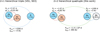 |
Fig. A.1. Schematic representation of the hierarchical configurations proposed for S1082. Left: the 2+1 model of V01 and S03, in which the close binary Aa–Ab (a ∼ 0.03 AU, e∼0; 2.52 and 1.58 M⊙) is orbited by a single blue straggler B (1.7 M⊙) on a wide, eccentric orbit (a∼4 AU, e∼0.57). Right: the 2+2 configuration favored in this work, consisting of two bound binaries: the close pair Aa–Ab (a = 0.02 AU, e = 0; 1.30 and 1.00 M⊙) and the wider Ba–Bb system (a∼3 AU, e∼0.58; 1.4 and 0.35 M⊙). These two binaries orbit each other on a very wide outer orbit with a = 390 AU. Orbits are not to scale; the schematic is intended only to illustrate the hierarchical architecture and labeling used throughout the paper. |
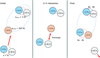 |
Fig. A.2. Schematic illustration of a possible 2+3 dynamical interaction leading to the present configuration of S1082. Left: Initial configuration, consisting of a wide quadruple in which the close pair Ba–Bb (1.4 and 0.35 M⊙; ainner ∼ 3 AU) orbits a 1.0 M⊙ star at aouter ∼ 390 AU. A separate binary with initial separation A1 (1.3 and 0.36 M⊙) approaches the system. This scenario assumes that prior MT within the incoming binary produced the BS before the encounter. Center: During the encounter, an exchange interaction occurs in which the 1.0 M⊙ star binds with the 1.3 M⊙ star from the incoming binary. Right: Final outcome, in which the interaction forms a close Aa–Ab binary (1.3 and 1.0 M⊙) and leaves the original Ba–Bb pair intact. The resulting two binaries remain gravitationally bound on a very wide orbit. Orbits are not to scale; the schematic is intended only to illustrate the dynamical exchange process discussed in Section 4.2.1. |
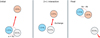 |
Fig. A.3. Schematic illustration of a possible 2+1 dynamical encounter leading to the formation of the close Aa–Ab binary in S1082. Left: Initial configuration, consisting of an approaching binary with initial separation A1 (1.3 and 0.4 M⊙) and an isolated 1.0 M⊙ star. This scenario assumes that prior MT within the incoming binary produced the BS before the encounter. Center: During the interaction, an exchange encounter occurs in which the 1.0 M⊙ star replaces the lower-mass component of the incoming binary. Right: Final outcome, producing the close Aa–Ab pair (1.3 and 1.0 M⊙) and ejecting the 0.4 M⊙ star. Orbits are not to scale; the schematic is intended only to illustrate the exchange process discussed in Section 4.2.2. |
Appendix B: Spectroscopic observations log
TRICOR radial velocities derived from TRES observations
CfA Radial velocities for S1082 B
All Tables
Initial orbital parameters from FEWBODY simulations used as input for MESA tidal circularization models, and the resulting final orbital period at 4 Gyr.
All Figures
|
Fig. 1. Light curves of S1082 phased to a period of 1.067795. Black dots are K2 (K2SFF) photometry after differential photometry and flattening, while blue dots are from TESS (QLP). |
| In the text | |
|
Fig. 2. Phased RV measurements for the eclipsing binary A, together with the RV curve for the orbital solution. Component Aa is shown as filled circles and component Ab as open circles. The orbital period used to phase the data is 1.067799 days. |
| In the text | |
|
Fig. 3. Phased RV measurements of the binary B, together with the RV curve for the orbital solution. The orbital period used to phase the data is 1184 days. |
| In the text | |
|
Fig. 4. Chosen “best segment” of the K2 C16 LC (black dots) and the best fit model (red line). The bottom panel shows the residuals from the fit. The orbital period used to phase the data is 1.067799 days. |
| In the text | |
|
Fig. 5. CMD of M67 showing the positions of the components of S1082. Gray points are confirmed cluster members from Geller et al. (2015b). A 4.0 Gyr MIST isochrone (dashed black line; 850 pc, AV = 0.093, solar metallicity) and single–star evolutionary tracks from 0.9–1.7 M⊙ are overplotted. Circles mark the component positions from Sandquist et al. (2003), while triangles show the updated values derived in this study (blue: Aa, 1.30 ± 0.13 M⊙, orange: Ab, 1.00 ± 0.07 M⊙). Red arrows mark the shifts from the earlier estimates to the new ones. |
| In the text | |
|
Fig. 6. O − C diagram of the times of the primary eclipse minima for S1082. We consider the same T0 as van den Berg et al. (2001), i.e., 2444643.25 HJD time. |
| In the text | |
|
Fig. 7. HR diagram showing the evolution of a representative conservative MESA mass transfer model, with initial masses of 1.23 M⊙ (donor, orange) and 1.07 M⊙ (accretor, blue), and initial orbital period of 0.95 days. Filled squares mark the observed positions of S1082 Aa and Ab. Circles show the model positions at 4 Gyr, crosses indicate when mass transfer begins, and diamonds mark the positions at 4.87 Gyr after mass transfer has altered both stars’ evolution. |
| In the text | |
|
Fig. 8. Relation between the final orbital period of the close binary ([2 3]) and the initial semimajor axis of the incoming binary (a1) in 2+3 encounters that resulted in a quadruple-single configuration. The best-fitting linear relation is shown in blue. The red vertical line marks the location of the observed orbital period of the close binary in S1082 (1.068 days). |
| In the text | |
|
Fig. 9. Relation between the final orbital period of the outer quadruple system ([[0 1][2 3]]) and the initial semimajor axis of the incoming binary (a1)in 2+3 encounters that resulted in a quadruple-single configuration. The red vertical line indicates a period of 1 × 10⁶ days, which is close to the orbital timescale inferred from the projected separation of the resolved components of S1082 (390 AU). |
| In the text | |
|
Fig. 10. Distribution of the final orbital periods and pericenter distances for all FEWBODY simulations that produced the desired [0 1] 2 binary-single outcome. |
| In the text | |
|
Fig. 11. Final orbital eccentricity vs. period for all FEWBODY simulations that produced the desired [0 1] 2 binary-single outcome with Pfinal < 100 days. Blue crosses show the subset of systems selected for MESA tidal circularization modeling. |
| In the text | |
|
Fig. A.1. Schematic representation of the hierarchical configurations proposed for S1082. Left: the 2+1 model of V01 and S03, in which the close binary Aa–Ab (a ∼ 0.03 AU, e∼0; 2.52 and 1.58 M⊙) is orbited by a single blue straggler B (1.7 M⊙) on a wide, eccentric orbit (a∼4 AU, e∼0.57). Right: the 2+2 configuration favored in this work, consisting of two bound binaries: the close pair Aa–Ab (a = 0.02 AU, e = 0; 1.30 and 1.00 M⊙) and the wider Ba–Bb system (a∼3 AU, e∼0.58; 1.4 and 0.35 M⊙). These two binaries orbit each other on a very wide outer orbit with a = 390 AU. Orbits are not to scale; the schematic is intended only to illustrate the hierarchical architecture and labeling used throughout the paper. |
| In the text | |
|
Fig. A.2. Schematic illustration of a possible 2+3 dynamical interaction leading to the present configuration of S1082. Left: Initial configuration, consisting of a wide quadruple in which the close pair Ba–Bb (1.4 and 0.35 M⊙; ainner ∼ 3 AU) orbits a 1.0 M⊙ star at aouter ∼ 390 AU. A separate binary with initial separation A1 (1.3 and 0.36 M⊙) approaches the system. This scenario assumes that prior MT within the incoming binary produced the BS before the encounter. Center: During the encounter, an exchange interaction occurs in which the 1.0 M⊙ star binds with the 1.3 M⊙ star from the incoming binary. Right: Final outcome, in which the interaction forms a close Aa–Ab binary (1.3 and 1.0 M⊙) and leaves the original Ba–Bb pair intact. The resulting two binaries remain gravitationally bound on a very wide orbit. Orbits are not to scale; the schematic is intended only to illustrate the dynamical exchange process discussed in Section 4.2.1. |
| In the text | |
|
Fig. A.3. Schematic illustration of a possible 2+1 dynamical encounter leading to the formation of the close Aa–Ab binary in S1082. Left: Initial configuration, consisting of an approaching binary with initial separation A1 (1.3 and 0.4 M⊙) and an isolated 1.0 M⊙ star. This scenario assumes that prior MT within the incoming binary produced the BS before the encounter. Center: During the interaction, an exchange encounter occurs in which the 1.0 M⊙ star replaces the lower-mass component of the incoming binary. Right: Final outcome, producing the close Aa–Ab pair (1.3 and 1.0 M⊙) and ejecting the 0.4 M⊙ star. Orbits are not to scale; the schematic is intended only to illustrate the exchange process discussed in Section 4.2.2. |
| In the text | |
Current usage metrics show cumulative count of Article Views (full-text article views including HTML views, PDF and ePub downloads, according to the available data) and Abstracts Views on Vision4Press platform.
Data correspond to usage on the plateform after 2015. The current usage metrics is available 48-96 hours after online publication and is updated daily on week days.
Initial download of the metrics may take a while.