| Issue |
A&A
Volume 706, February 2026
|
|
|---|---|---|
| Article Number | A327 | |
| Number of page(s) | 10 | |
| Section | Stellar structure and evolution | |
| DOI | https://doi.org/10.1051/0004-6361/202557545 | |
| Published online | 17 February 2026 | |
Luminous fast blue optical transients as very massive star core-collapse events
1
European Space Agency (ESA), European Space Research and Technology Centre (ESTEC) Keplerlaan 1 2201 AZ Noordwijk, The Netherlands
2
Department of Astrophysics/IMAPP, Radboud University PO Box 9010 6500 GL Nijmegen, The Netherlands
3
Department of Physics, University of Warwick Gibbet Hill Road CV4 7AL Coventry, United Kingdom
4
School of Natural Sciences, Institute for Advanced Study 1 Einstein Drive Princeton NJ 08540, USA
★★ Corresponding author: This email address is being protected from spambots. You need JavaScript enabled to view it.
Received:
3
October
2025
Accepted:
29
December
2025
Abstract
Context. Luminous fast blue optical transients (LFBOTs) are rare extragalactic events of unknown origin. Tidal disruption events (TDEs) involving white dwarfs by intermediate mass black holes (BHs), mergers of BHs and Wolf-Rayet (WR) stars, and failed supernovae (SNe) are among the proposed explanations.
Aims. In this paper, we explore the viability of very massive star core-collapse (CC) events as the origin of LFBOTs. The appeal of such a model is that the formation of massive BHs via CC events could yield observational signatures that can match the disparate lines of evidence that point towards both CC and TDE origins for LFBOTs.
Methods. We explored the formation rate of massive BHs in binary population synthesis models and compared the metallicities of their progenitors with the observed metallicities of LFBOT host galaxies. We further examined the composition, mass-loss rates, and fallback masses of these stars, placing them in the context of LFBOT observations.
Results. We determined the formation rate of BHs with masses greater than ∼30–40 M⊙ to be similar to the observed LFBOT rate. The stars producing these BHs are biased towards a low metallicity (Z < 0.3 Z⊙) and they are H- and He-poor, with dense circumstellar media. However, some LFBOTs have host galaxies with higher metallicities than predicted and they typically have denser local environments (plausibly due to late stage mass loss not captured in the models). We find that long-lived emission from an accretion disc (as implicated in the prototypical LFBOT AT 2018cow) can only be produced in these events under maximal disc mass and angular momentum conditions.
Conclusions. We conclude that a (very) massive star CC scenario is a plausible explanation for at least some LFBOTs, but it still faces challenges. The preferred progenitors for LFBOTs in the failed SN interpretation overlap with those predicted to produce super-kilonovae (super-KNe). We therefore suggest that LFBOTs are promising targets in the search for super-KNe and that they could offer a non-negligible contribution to the r-process enrichment of galaxies.
Key words: stars: black holes / stars: massive / supernovae: general
ESA Research Fellow.
© The Authors 2026
 Open Access article, published by EDP Sciences, under the terms of the Creative Commons Attribution License (https://creativecommons.org/licenses/by/4.0), which permits unrestricted use, distribution, and reproduction in any medium, provided the original work is properly cited.
This article is published in open access under the Subscribe to Open model. This email address is being protected from spambots. You need JavaScript enabled to view it. to support open access publication.
1. Introduction
Luminous fast blue optical transients (LFBOTs), also known as Cow-like transients after the prototypical AT 2018cow (Prentice et al. 2018; Perley et al. 2019), are rapidly evolving transients with peak optical-ultraviolet (optical-UV) luminosities rivalling super-luminous supernovae (SLSNe). Their early optical-UV spectra are well described by a hot, featureless blackbody (T > 20 000 K), lacking H and He lines initially. They have decay rates of ≳0.3 magnitudes per day, ruling out any significant contribution from 56Ni-powered emission. They are also accompanied by bright X-ray (and, at late times, radio) emission. The late-time radio emission is attributed to self-absorbed synchrotron emission from an expanding blast wave in a dense circumstellar medium (CSM).
A modest sample of LFBOTs has now been identified in addition to AT 2018cow: ZTF18abvkwla (AT2018lug, Ho et al. 2020), CSS161010 (Coppejans et al. 2020; Gutiérrez et al. 2024), ZTF20acigmel (AT2020xnd, Perley et al. 2021; Bright et al. 2022), AT2020mrf (Yao et al. 2022), AT2022tsd (Matthews et al. 2023), AT2023fhn (Chrimes et al. 2024a,b), and AT2024wpp (Pursiainen et al. 2025; Nayana et al. 2025), along with the slower evolving and radio-faint (but otherwise similar) AT2024puz (Somalwar et al. 2025) and several other candidates that lack extensive multi-wavelength follow-up. Some transients display very blue colours, evolve rapidly at early times, and produce bright X-ray emission, similarly to LFBOTs, but are followed by broad lined type Ic SNe (e.g. the Einstein Probe-discovered transients EP2404014A and EP250108A, van Dalen et al. 2025; Eyles-Ferris et al. 2025; Rastinejad et al. 2025). However, these events likely do not share the same progenitors as LFBOTs, given that they successfully launched SNe. Therefore, here we focus solely on the SN-less, Cow-like LFBOTs, whose origins remain unknown. The volumetric rate of LFBOTs is estimated to be ∼0.1% of the core-collapse (CC) SN rate (Ho et al. 2023b).
Two categories of model to explain LFBOTs have emerged as most likely (e.g. Perley et al. 2019). The first invokes tidal disruption events (TDEs) of H- and He-poor, compact stars (e.g. a white dwarf) by intermediate-mass black holes (IMBHs, Kuin et al. 2019). This model faces challenges primarily due to the dense CSM observed in LFBOTs. Although such a environment is possible in TDEs involving stars disrupted by supermassive black holes (SMBHs), it is less clear whether white dwarf plus IMBH TDEs could produce similar circumstellar density profiles (Margutti et al. 2019; Linial & Quataert 2024). The second category of proposals are broadly themed around stellar mass BH accretion, either in mergers or collisions (Metzger 2022; Grichener 2025; Tsuna & Lu 2025; Klencki & Metzger 2025) or CC events (e.g. Kashiyama & Quataert 2015; Margutti et al. 2019; Quataert et al. 2019; Gottlieb et al. 2022).
We know that at least some sufficiently massive stars are expected to directly form BHs without launching a SN. The landscape of explodability is thought to be complex, with neutron star and some BH-forming events capable of launching successful SNe, and other BH-forming CC events resulting in direct BH formation without any significant ejecta (e.g. Heger et al. 2003; Ertl et al. 2020). Observational evidence of ‘quiet’ BH formation comes from a lack of massive stars ≳20 M⊙ in pre-SNe imaging, and the disappearance of supergiant stars without any evidence of a SN (Smartt et al. 2009; Williams et al. 2014; Reynolds et al. 2015; Adams et al. 2017b,a; Beasor et al. 2024).
Some LFBOT models invoke such a scenario, where a massive star collapses to a BH without a successful SN (i.e. a ‘failed SN’), followed by the accretion of some fraction of the remaining (‘leftover’) material onto the nascent BH (e.g. Perna et al. 2014; Kashiyama & Quataert 2015; Fernández et al. 2018; Quataert et al. 2019). The failed SN hypothesis resembles early collapsar gamma-ray burst (GRB) models (e.g. Woosley 1993; MacFadyen & Woosley 1999; Fryer et al. 1999), which also feature accreting BHs born in CC events, but without a successful (or a weak) SN. In LFBOTs there is no evidence of a SN, but unlike the case of collapsar GRBs, no gamma-ray emission has been observed and the outflows are only mildly relativistic (e.g. Coppejans et al. 2020).
Altough some fast-evolving optical transients can be explained solely with circumstellar interactions (Pellegrino et al. 2022), in the case of LFBOTs there is evidence of central engine activity. AT 2018cow showed short timescale variability in its light curve (Ho et al. 2019; Margutti et al. 2019; Pasham et al. 2021), as well as UV and X-ray emission lasting at least several years post-explosion (Sun et al. 2022, 2023; Inkenhaag et al. 2023; Chen et al. 2023; Migliori et al. 2024; Inkenhaag et al. 2025). Magnetar central engines have been proposed as an explanation (Fang et al. 2019; Mohan et al. 2020; Liu et al. 2022; Li et al. 2024), but they struggle to reconcile both the early-time emission and late-time optical/UV plateau (Chen et al. 2023). Assuming instead that LFBOTs are BH-powered, estimates for the BH mass in such a scenario have been derived from quasi period oscillations (Pasham et al. 2021) and accretion disc modelling (Inkenhaag et al. 2023; Migliori et al. 2024; Cao et al. 2024; Inkenhaag et al. 2025) yielding masses that span the upper end of the stellar mass BH distribution into the intermediate-BH mass regime. The observation of late-time, short duration giant optical flares from AT 2022tsd (Ho et al. 2023a) could also be consistent with a highly variable accretion rate, either around the BH formed in the event or a companion BH (Lazzati et al. 2024). Similar flaring behaviour has not been found in AT20224wpp (Ofek et al. 2025).
The BH mass estimates for LFBOTs are high and they have been discovered thus far in non-nuclear regions of low-metallicity, star-forming galaxies. The aim of this paper is to explore other observational consequences (e.g. in terms of volumetric rates and the metallicities of their hosts) if LFBOTs are indeed powered by massive BH formation in failed SNe. In Section 2, we compare population synthesis predictions for the rate of BH formation as a function of mass with the observed LFBOT rate. In Section 3, we investigate whether the metallicity bias associated with the formation of the most massive stellar mass BHs is consistent with LFBOT environments. We explore in Section 4 whether the selected stellar models can plausibly reproduce the key characteristics of LFBOT emission, with a discussion and conclusions following in Sections 5 and 6.
2. BH formation and LFBOT event rates
We first considered what the volumetric formation rate of stellar-mass, CCBHs with masses > MBH, min would be and what value of MBH, min would best reproduce the LFBOT rate. To explore these questions, we coupled a population synthesis with a model for the metallicity-dependent cosmic star formation rate history.
For the population synthesis, we used the Binary Population and Spectral Synthesis (BPASS) models (v2.2.1, Eldridge et al. 2017; Stanway & Eldridge 2018), comprised of a publicly available grid of pre-calculated binary stellar evolution models where the primary evolution is followed in detail, while the secondary is evolved with the rapid evolution prescriptions of Hurley et al. (2002). Models are provided at 13 metallicities and at each metallicity, each stellar model is weighted according to observed binary parameter distributions (Moe & Di Stefano 2017). We adopted the model set with a Kroupa (2001) broken power-law initial mass function (IMF), with a minimum mass of 0.1 M⊙ and a maximum of 300 M⊙, a break mass of 0.5 M⊙, and a slope of α = −1.30 (−2.35) below (above) the break. At each metallicity, Z, the weighting of each model corresponds to the number of systems resembling that model expected in a stellar population of 106 M⊙. For more details on the binary stellar models and the code, we refer to the BPASS v2 release paper Eldridge et al. (2017).
For the metallicity-dependent cosmic star formation rate history, CSFH(Z, z), we adopted the model of Langer & Norman (2006). We seeded the population synthesis models according to this CSFH, such that the volumetric birth rate of each system (BPASS model) at each redshift, z, and metallicity, Z, is proportional to the product of the star formation rate density, SFRD(Z, z), and the model weighting (defined by the IMF and binary parameter distributions as described above).
We adopted the standard BPASS assumptions that a CC event occurs when, at the end of the model, the total mass exceeds 1.5 M⊙, the CO core mass exceeds 1.38 M⊙ and the ONe core mass is non-zero. Remnant masses are a pre-calculated output of the models. They are determined by injecting 1051 erg of energy, calculating the mass in the outer layers that can be lifted to infinity by this energy injection, and taking the remaining mass as the remnant mass (for more details, see Eldridge & Tout 2004; Eldridge et al. 2017). We note that this energy injection is likely an overestimate for BH-forming events and means we have a large amount of mass potentially available for fallback accretion (addressed later in this paper). We classified all CC remnants with M < 3 M⊙ as neutron stars (NSs), and those heavier as BHs. We assumed that all NS-forming events produce successful SNe and that BH-forming events do not. Pair-instability SNe (PISNe) are deemed to occur if the final carbon-oxygen core mass exceeds 60 M⊙ and the final helium core mass is < 133 M⊙. In this case no remnant is left behind (Heger & Woosley 2002). Pulsational PISNe (PPISNe) are accounted for by adopting the remnant mass prescription of Farmer et al. (2019) for final carbon-oxygen masses between 38 and 60 M⊙, following Briel et al. (2023). The true landscape of explodability and remnant formation is more complex and our assumptions neglect islands of explodability above the mass regime where neutron stars are formed, but capture the broad behaviour predicted by many works (e.g. Smartt et al. 2009; Smartt 2009; Fryer et al. 2012; Ertl et al. 2020; Sukhbold & Adams 2020; Patton & Sukhbold 2020; Kresse et al. 2021; Patton et al. 2022; Laplace et al. 2025; Ugolini et al. 2025; Maltsev et al. 2025). These assumptions also naturally reproduce observed (binary) remnant mass distributions (e.g. Kochanek 2014; Briel et al. 2023; Disberg & Nelemans 2023; The LIGO Scientific Collaboration 2025). Nevertheless, we acknowledge the possible impacts of these simplifying assumptions in Section 5.3.
The remnant formation time for each stellar model is the seed time, plus the age of the model at CC (although for these short-lived stars, this is negligible compared with cosmological timescales). In this way, we were able to construct a metallicity-weighted SN rate and BH formation rate as a function of redshift. Since we found that all (confirmed) LFBOTs thus far had redshifts of z < 0.4, we compared the mean rate of SNe and BH-forming events over this redshift range for different values of MBH, min. Specifically, we calculate the mean ratio of the SN rate and the formation rate of BHs with mass MBH, min or greater. As the form of CSFH(Z, z) is uncertain, we repeat the process with two extreme variations of the CSFH(Z, z). These are defined by shifting the Langer & Norman (2006) model by ±0.2 dex in 12+log(O/H), which captures the approximate envelope of possible CSFHs found by Chruslinska & Nelemans (2019).
The results are shown in Figure 1. Using the fiducial CSFH we find that the birth rate of BHs at z < 0.4 with masses ≳38 M⊙ is ∼0.1% of the CCSN rate, matching that of the LFBOTs. The progenitor temperatures, luminosities, and radii prior to collapse are provided in Figure A.1 of Appendix A. For a CSFH of the same form but peaking at a metallicity 0.2 dex lower in 12+log(O/H), we find that a higher BH mass threshold of ≳41 M⊙ is required because there are more high-mass BHs being formed overall with respect to CCSNe. The reverse is true for a CSFH, which peaks 0.2 dex higher, yielding a threshold of ≳33 M⊙. Therefore, varying the CSFH changes the absolute number of BHs being born (although not the general shape of the BH mass distribution, van Son et al. 2023) and the number formed with respect to CCSNe.
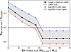 |
Fig. 1. Mean ratio of the rate of BH formation above a minimum mass, MBH, min, to the rate of CC SNe at z < 0.4. The black line shows this ratio as a function of MBH, min assuming the metallicity-dependence cosmic star-formation history (CSFH) of Langer & Norman (2006). The red and blue lines, bounding the grey shaded region, are the result of adopting a CSFH shifted up/down by 0.2 dex in 12+log(O/H), respectively. The horizontal dashed line is the estimated LFBOT volumetric rate (Ho et al. 2023b). We therefore find that the predicted formation rate of BHs with masses greater than (38 |

Above mass cuts of ∼45 M⊙, the ratio of birth rates remains constant, because the cut has moved into the PISN mass gap and only BHs with masses above the gap are contributing. In summary, we find that the birth rate of BHs heavier than several tens of solar masses is similar to the LFBOT rate and that this result is robust against uncertainties in the CSFH.
3. Metallicity dependence and LFBOT host galaxies
Given a BH mass cut MBH, min, which yields a BH formation rate matching the observed LFBOT rate, for an assumed CSFH, in the next step, we can consider what the (CSFH weighted) metallicity distribution of the progenitors of these BHs would be and how it would compare to the host galaxies of LFBOTs. We collate the available information in the literature on LFBOT host metallicities in Table 1. Four of the seven have host-averaged metallicities derived from spectral energy distribution (SED) fitting. In one case (AT 2018cow), there are available integral field unit data, enabling a more local (resolution of a few hundred parsec, Lyman et al. 2020) measurement of the metallicity. For the remaining two, no direct measurement has been published, so we obtained an approximate value through the galaxy mass-metallicity relation (Tremonti et al. 2004). We adopted Z⊙ = 0.02 by mass fraction for solar metallicity, but we note that this specific choice has no impact on the comparisons or analysis since both the observed and synthetic metallicities were scaled by the same factor.
LFBOTs, their host metallicities, and references.
In Figure 2, we compare the number of BHs more massive than MBH, min born per 106 M⊙ of star formation, weighted by the mean z < 0.4 metallicity distribution for each of the three CSFHs adopted, along with the measured distribution of LFBOT host or environmental metallicities. There is a strong preference for BHs with masses greater than 38 M⊙ to be born in stellar populations with a metallicity of less than ∼0.3 Z⊙. Below this threshold, the distributions are relatively constant: this reflects that the fact that (i) we are tailoring our mass cut to yield a BH formation rate that is 0.1% of the CCSN rate for each CSFH and (ii) that the CCSN rate itself is not substantially varying with the CSFH variations. This is because NS formation efficiency (unlike BH formation efficiency) does not sharply decline at higher metallicities (e.g. van Son et al. 2025).
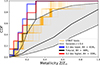 |
Fig. 2. Cumulative distribution of LFBOT host galaxy metallicities is shown in orange (see Table 1). We sample the Z values, assuming Gaussian uncertainties, 100 times, producing the many realisations of the cumulative distribution shown. Cumulative distributions of our selected progenitor metallicities, weighted by the CSFH(Z) at z < 0.4, are also shown. The black line is the z < 0.4 mean metallicity distribution of star-forming galaxies Langer & Norman (2006). The grey shaded region bounded by dashed lines is defined by shifting the distribution of Langer & Norman (2006) by ±0.2 in 12+log10(OH), covering the high- and low-Z extremes defined by Chruslinska & Nelemans (2019). |
It is immediately apparent that LFBOT environments sample the Z ≲ 0.5 Z⊙ region. The formation of BHs with M > MBH, min across this range instead samples metallicities of Z < 0.3 Z⊙. A KS-test between the LFBOT host values and the fiducial > 38 M⊙Z distribution returns p = 0.01, formally rejecting the null hypothesis that the observed host values are consistent with the synthetic distribution. However, we note that the host metallicities are far from uniformly determined, with methods ranging from resolved IFU spectroscopy probing the local environment within the host to host-integrated metallicities to the mass-metallicity relation. This likely introduces errors and scatter that have not been accounted for; thus, host-integrated measurements will naturally be higher than the lowest metallicity environments within each host. There might also be pockets of low-metallicity gas within and around star-forming galaxies, driving low-Z star-formation (e.g. Michałowski et al. 2015; Metha & Trenti 2023). Nevertheless, the current information suggesting that LFBOTs can occur in environments with metallicities above the strong cut-off predicted is a challenge to the model. This is most notable for AT2018cow, whose metallicity measurement is integrated across the immediate (few hundred pc) environment (Lyman et al. 2020), but even in this case variations on smaller scales are possible.
4. Expectations for the emission
4.1. H and He-poor spectra
LFBOTs display H and He poor spectra at early times (e.g. Prentice et al. 2018). The progenitor star (or the star undergoing a TDE) must therefore have a H- or He-poor composition. In the TDE scenario, a white dwarf is favoured (Kuin et al. 2019). For a BH-stellar merger, the stellar object must be a Wolf-Rayet (WR) star (Metzger 2022). In the scenario explored in this paper, the median H and He mass fractions in the ‘leftover mass’1 of the models selected as progenitors of BHs with M > 38 M⊙ are, respectively,  and Ysurf = 0.08
 , where the uncertainties are defined by the 16th and 84th percentiles). The distributions of Xsurf and Ysurf are shown in Figure 3. Overall, 69% of our selected models are classified as WR stars given the Xsurf values and high surface temperatures of log10(T/K) > 4.45 (Eldridge et al. 2017). The outer layers of these stars therefore meet the criteria for being H- and He-poor and successfully exploding stars with such low X and Y surface mass fractions are expected to produce type Ic SNe (i.e. SNe without detectable H and He lines, e.g. Dessart et al. 2012; Eldridge et al. 2013; Chrimes et al. 2020).
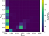 |
Fig. 3. Leftover (i.e. ejected and/or accreted) mass fractions of hydrogen (Xsurf) and helium (Ysurf) in the last time-step of the selected BPASS models, with contributions from different metallicities determined by the mean metallicity spread at z < 0.4 (Langer & Norman 2006). The colourbar indicates the number of events per 106 M⊙ of star formation, with contributions from different metallicities following the fiducial case as shown in Figure 2, along with the model weightings as defined in Section 2. |
4.2. Dense circumstellar media and radio emission
A key characteristic of LFBOTs is their slow-rising, luminous radio emission, attributed to self-absorbed synchrotron emission from a blast wave expanding through the circumstellar medium (CSM). These blast waves are mildly relativistic (e.g. Coppejans et al. 2020), enabling us to probe the CSM at radii of ∼1016–1017 cm. LFBOT radio emission is well described by blast-wave propagation through dense CSM profiles defined by Ṁ/Vw values of ∼1–100, in units of 10−4 M⊙ yr−1/1000 km s−1. For WR wind speeds of order 1000 km s−1, radii of ∼1016–1017 cm corresponds to mass loss in the final decades before explosion. We calculated the mean final Ṁ/Vw values for the selected models, noting that BPASS only runs until the end of core carbon burning. The mass-loss rates are provided as a BPASS output. We adopted standard BPASS wind speed prescriptions, namely those of Vink et al. (2001), and Nugis & Lamers (2000) for WR stars (we refer to Eldridge et al. 2017; Chrimes et al. 2022, for more details). We found a median final result of Ṁ/Vw = (0.04 ) 10−4 M⊙ yr−1/1000 km s−1. The full distribution of Ṁ/Vw is shown in Figure 5. The bulk of our progenitor mass-loss rate and wind speed values lie below the values inferred from LFBOT radio observations, which span the range ∼1–100 in these units (e.g. Ho et al. 2022; Bright et al. 2022, under the assumption of ϵe = 0.1 and ϵB = 0.01). We note that mass loss in the final decades before CC could be significant and eruptive, plausibly explaining the non-r−2 profiles observed (e.g. Smith 2014). However, because the stellar evolution models used end after core carbon burning, a full modelling of the CSM around these stars on the relevant scales is beyond the scope of this paper.
4.3. Long-lived UV plateaus
Finally, we ask whether the selected stellar models can produce a long-lived tail of UV emission lasting at least several years after the event, as observed in AT2108cow (Sun et al. 2022, 2023; Chen et al. 2023; Inkenhaag et al. 2023, 2025). This has been interpreted as due to a long-lived accretion disc, reminiscent of the emission seen in TDEs (Metzger 2022; Inkenhaag et al. 2023; Mummery & van Velzen 2025). To see whether our models can produce AT 2018cow-like UV plateaus through this mechanism, we first examined the remaining mass in the selected BPASS models that survives outside the nascent BHs (i.e. the pre-CC mass minus the initial BH mass). In Figure 4, we show 2D histograms of these masses at each metallicity, for the fiducial Langer & Norman (2006) CSFH. For more details on the BH mass distribution in BPASS, we refer to Eldridge et al. (2017), Ghodla et al. (2022) and Briel et al. (2023). More details on the progenitors, in terms of temperature, luminosity, and radius at the end of the models (i.e. the end of core carbon burning) are given in Appendix A.
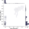 |
Fig. 4. Remnant BH mass versus the ‘leftover’ mass for the models selected when the fiducial CSFH is used (black lines in Figures 1 and 2). These are the remnant and leftover (ejecta) masses when an CC energy injection of 1051 erg is assumed (Eldridge & Tout 2004), taking into account the mass gap from PISNe and PPISNe (Farmer et al. 2019; Briel et al. 2023). The histograms show the number events expected per 106 M⊙ of star formation, as described in Figure 3. |
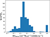 |
Fig. 5. Wind density parameter for the selected models, normalised by a typical WR mass-loss rate and wind speed. The circumstellar densities resulting from these values are lower than typical WR stars and lower than observed in some LFBOTs, likely due to weaker winds as a result of the strong low-metallicity bias introduced by requiring such massive BHs. Typical LFBOT values are in the range 1–100 (e.g. Ho et al. 2022; Bright et al. 2022). The y-axis indicates the number events per 106 M⊙ of star formation, as described in Figure 3. |
As outlined in Section 2, BPASS calculates BH masses by injecting a standard SN energy of 1051 erg to determine the mass of the material that is unbound. The remainder is then the remnant mass. In a failed SN, the ‘leftover’ material is not successfully ejected. It might therefore be reasonable to assume that all of the leftover material falls back and is accreted instead, in line with other prescriptions for final BH masses in the massive to very massive star regime, which have close to a one-to-one relation between the pre-CC mass and final remnant mass (after fallback) for stripped envelope progenitors (Fryer et al. 2012; Briel et al. 2023). With the BH mass, MBH, leftover mass, Mleftover, total pre-collapse stellar mass, M★, radius, R★ and rotational velocity, v★ as inputs, we can determine an initial disc radius, r0, as follows,
 (1)
(1)
where fj, disc and facc are the fraction of the pre-collapse angular momentum and leftover mass which go into the disc, respectively. A derivation of Equation (1) is provided in Appendix B. Since stellar rotation is not explicitly tracked in BPASS, we have assumed the pre-collapse rotational velocity to be 10% of the breakup (critical) velocity. We note that massive stars in low-metallicity environments (e.g. the Magellanic Clouds) are observed to be rotating at ∼10–20% of their critical velocity (e.g. Ramírez-Agudelo et al. 2013, 2015). We proceeded to use the model of Mummery & Balbus (2020), Mummery et al. (2025) to calculate UV light curves for every selected stellar model. The final parameter required (beyond the disc mass, BH mass and radial scale) is the initial evolutionary timescale of the disc. We follow standard Shakura & Sunyaev (1973) theory and take  , where α ∼ 0.1 is a dimensionless factor, and θ ≡ h/r is the disc aspect ratio. Anticipating a thick disc (for this likely initially super-Eddington flow), we sampled α−1θ−2 in the range ∼(50, 500), inducing scatter in our simulated light curves. This allows us to fix all the parameters in the disc model.
We adopted two example scenarios, showing the predicted UV light curves in Figure 6 for the F225W Wide Field Camera 3 (WFC3) Hubble Space Telescope filter. In first two, only 10% of the available angular momentum and mass is transferred to the disc. In the second extreme case, all of the angular momentum and mass goes into the disc. We acknowledge that the details details of SN fallback, such as its asphericity and the fraction that falls back versus being ejected, are not captured in the models or our simple parametrisation. This motivated our choice of two scenarios which nevertheless represent a wide range of possible fallback masses and angular momenta, including the hypothetical ’maximum’ case. The total leftover mass is also uncertain (and depends on the injected energy at CC). For a discussion of the impact of this we refer to Section 5.3.
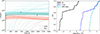 |
Fig. 6. Left: Predictions for UV light curves arising from the accretion disc around natal BHs of mass greater than 38 M⊙ in our failed SN models, using the model of Mummery & Balbus (2020), Mummery et al. (2025). These predictions are for observations in the Hubble Space Telescope WFC3/F225W filter; the black points are late-time F225W observations of AT 2018cow (Inkenhaag et al. 2023). Two example cases are shown: one assuming that 10% of the total pre-collapse angular momentum and 10% of the leftover mass, goes into the disc (red). The other is the extreme case that 100% of the available angular momentum and mass goes into the disc (cyan). Both scenarios adopt progenitor rotation at 10% of the critical velocity. The large spread in luminosity in both the cyan and red curves is due to the spread in BH and leftover masses (spanning the pair instability mass gap, see Figure 4). Right: Disc radii for the fiducial selected models at t = 0, 1, and 1000 days. The radii are the same for both the 10% and 100% assumptions (see Equation 1). The discs spread rapidly, with around 40% of them reaching radii of 30–40 R⊙ within the first day (the scale inferred from blackbody modelling of LFBOT observations). All discs ultimately reach 100–1000 R⊙ by 1000 days. |
The resulting light curves can only match the observed late-time F225W flux for AT 2018cow if a large fraction of the leftover mass and angular momentum are transferred to the disc (see also Omand et al. 2026). The initial disc radii predicted from these models are considerably smaller than the ∼30–40 R⊙ inferred from the late-time fits to AT2018cow (Inkenhaag et al. 2023; Migliori et al. 2024). This is because the majority of the progenitors are compact stars (e.g. WR stars; see Figure A.1 of Appendix A). However, the discs spread rapidly (as t2/3), reaching ∼10 R⊙ within a day and ∼100 R⊙ within 1000 days. We note that the factors facc and fj, disc cancel out, so that the two cases adopted return the same initial disc radii. The growth of the outer disc radius will be less pronounced if angular momentum is transported away from the disc by winds (potentially likely at early times), as detailed in Appendix B. We find that tvisc covers a wide range of ∼0.5–106 days. It is only for the shortest of these timescales that the same accretion mechanism could plausibly explain the rapid early-time rise in LFBOT light curves. Otherwise, we acknowledge that some other process must be driving the initial rise and peak.
The failed SN interpretation of LFBOTs is predicated on the notion that some non-negligible fraction of the total stellar mass does not participate in the prompt BH formation and instead falls back onto the nascent BH. If the CC of such massive stars actually results in the entire stellar mass being promptly engulfed by the event horizon, there will no material to accrete, ruling out failed SNe as a viable channel for LFBOTs. However, in our fiducial models this is not the case (see Figure 4, as well as a discussion of the explodability assumptions in Section 5.3).
5. Discussion
5.1. LFBOT environments
In the failed SN scenario, we would expect LFBOTs to be strongly associated with star-forming regions, as the short-lived massive progenitors are not expected to travel far from their birth sites. Although the LFBOT sample is small, it appears as though LFBOTs occupy diverse environments within their hosts, with at least two events at moderate-to-large host-normalised offsets (Chrimes et al. 2024b; Pursiainen et al. 2025). The apparent preference for LFBOTs to occur in low-metallicity environments might help in this regard: in general, galactic outskirts have a lower metallicity than their inner regions (e.g. Pilkington et al. 2012; Ju et al. 2025). However, a similar argument could be made for such events as, for instance, CC gamma-ray bursts, which are not typically observed at large offsets. Regardless of offsets, the host metallicities of LFBOTs extend above the sharp cut-off predicted for CC events involving very massive stars (see Sect. 3). Furthermore, metallicities from SED fitting should be treated with caution (e.g. Nersesian et al. 2025). For example, the mass-metallicity relation for the host of AT 2023fhn suggests a metallicity of ∼0.5 Z⊙, versus the fitted value of ∼0.1 Z⊙. In any case, the metallicity distributions as presented in Fig. 2 are inconsistent, but the possibility of low-Z pockets on spatial scales smaller than probed by current measurements has the potential to resolve this discrepancy.
5.2. Initial mass function
We have adopted model weightings with an initial mass function (IMF) slope above 0.5 M⊙ of −2.35. Two other high-end slopes are available with the BPASS outputs: −2.00 and −2.70. If the −2.70 slope is adopted, fewer high-mass BHs are born and the cut-off MBH, min drops to ∼30 M⊙, such that the BH formation rate remains consistent with the LFBOT rate (0.1% of the CCSN rate). The number of neutron star progenitors also decreases, such that the SN rate decreases, reducing the amount by which MBH, min has to decrease in order to maintain 0.1% of the CCSN rate. If −2.00 is adopted, there are more BHs and the cut-off moves up to ∼40 M⊙, around the lower edge of the PISN mass gap. This range (i.e. ∼30–40 M⊙) represents the uncertainty in the minimum BH mass required to match the LFBOT rate, which arises from the choice of IMF. This is slightly larger than the uncertainty arising solely from the choice of CSFH(Z, z). Nevertheless, the broad conclusion is that the formation rate of BHs with masses greater than ∼30–40 M⊙ is consistent with the LFBOT rate.
5.3. Explodability and remnant mass assumptions
The results in this paper depend on the BH masses formed and the mass available in the ‘leftover’ material for fallback. The models adopted calculated BH masses by injecting 1051 erg of energy and determining the mass which which remains bound. If the actual energy injection in failed events is ≪1051 erg (as expected, e.g. Fernández et al. 2018; Kuroda & Shibata 2023) then the BH masses will be greater. However, the ejecta and leftover masses are typically not more than 10% of the BH mass, so the most they could increase by is about ten times, which would not significantly change our conclusions. Ultimately, the models predict similar final remnant masses to other widely used prescriptions in the high-mass regime (e.g. Fryer et al. 2012, see also Figure A.2 of Appendix A).
There is also the question of which stars explode and which undergo a failed collapse. Our assumption that all BH-forming events fail is an upper limit on the rate of failed SNe. The predicted rate of all failed SNe under this assumption is ∼0.2 of the CCSN (or NS) formation rate, which is compatible with upper limits on the rate of failed SNe from searches for faint, long-lived red transients (thought to be a likely outcome for failed SNe in the absence of any additional energy injection from a disc, Byrne & Fraser 2022).
However, we are likely overestimating the failed SN rate, given recent hydrodynamical simulations and suggestions that there may not be a missing red supergiant problem (e.g. Burrows et al. 2025; Beasor et al. 2025). If failed SNe only occur in the 12–15 M⊙ (ZAMS mass) window where failed events are reliably predicted to occur in these simulation (and assuming NS formation everywhere outside this range unless a PISN occurs), then we would expect a ratio of failed events to CCSNe of ∼0.15. The lower masses (higher up the IMF) counteract the narrower mass range, producing a similar ratio to our fiducial > 30–40 M⊙ BH mass cut. Such a scenario could therefore reproduce the LFBOT rate but not the inferred BH masses. The prospect of incorporating more physically motivated prescriptions for remnant and ejecta mass distributions in the framework of population synthesis (e.g. Patton & Sukhbold 2020; Maltsev et al. 2025) could help refine results such as these in future.
5.4. A potential source of r-process nucleosynthesis
Massive BHs and their accretion discs, such as those discussed here, have also been predicted as possible sites of ‘super-kilonovae’ (super-KNe). In this scenario, the density in a high Ṁ accretion disc becomes high enough to trigger r-process nucleosynthesis (Siegel et al. 2019, 2022; Dean & Fernández 2024; Rastinejad et al. 2024; Agarwal et al. 2026). The possibility of such a channel has implications for where and when r-process elements are produced in the Universe (Nugent et al. 2025). Given the BH and accreted masses involved in the failed SN interpretation of LFBOTs, they may be promising sites for r-process production. The volumetric rate of LFBOTs in the redshift range considered in this work (Ho et al. 2023b, 0.1% of the CCSN rate, or 70 yr−1 Gpc−3) is compatible with the rate of super-KNe predicted by Siegel et al. (2022) of 10–100 yr−1 Gpc−3. We have shown that the failed-SN interpretation of LFBOTs naturally favours events forming BHs greater than 30 − 40 M⊙, while super-KNe have been predicted in events producing BHs greater than ∼60 M⊙ (Siegel et al. 2022). If the true rate of LFBOTs is just a factor of few lower than the current (≲70 yr−1 Gpc−3) best estimate, then the BH mass cut required to match the LFBOT rate moves up to the pair instability mass gap (see Figure 1) and we have a 1:1 mapping between LFBOT and super-KN progenitors. In any case, there is surely substantial overlap in the populations. Furthermore, a near-infrared excess (a hallmark of radiative reprocessing by r-process elements) was observed on a timescale of weeks following both AT 2018cow (Perley et al. 2019) and AT2024wpp (Pursiainen et al. 2025). This has been described either as a dust echo or due to free-free opacity effects outside the optical photosphere in both events (Metzger & Perley 2023; Nayana et al. 2025), but no spectroscopic characterisation of this feature in an LFBOT has yet been obtained. Future near-infrared spectroscopic observations (e.g. JWST) could potentially distinguish between an r-process element-forming super-KN and a featureless dust echo or free-free emission. However, in order for a UV-emitting disc and IR-emitting super-KN to be simultaneously observable, an anisotropic geometry that allows for a simultaneous viewing of both photospheres would be required.
5.5. Further implications
There are several other observations associated with LFBOTs that must be satisfied by any model invoked to explain them, assuming that LFBOTs are homogenous class. For example, extremely high-velocity (v = 0.1c), blue-shifted hydrogen lines were observed in the CSS161010 (Gutiérrez et al. 2024). This are perhaps most easily explained as out-flowing streams of material in a TDE, although they have only been observed in CSS161010 thus far. Polarimetric observations have found that LFBOTs start highly polarised and display a trend towards low polarisation on a timescale of days (Maund et al. 2023; Pursiainen et al. 2025). This can plausibly be explained in a failed-SN scenario by (i) an accretion disc producing the high early-time polarisation and (ii) a rapid transition to an spherical outflow (Pursiainen et al. 2025), perhaps caused by outflows from highly super-Eddington accretion (e.g. Coppejans et al. 2020). The origin of the giant optical flares observed from AT2022tsd in the months after the event is unclear, but timescale arguments constrain the scale of the emitting region to the outer regions of an accretion disc for a stellar-to-intermediate-mass BH’s central engine (Ho et al. 2023a).
6. Conclusions
In this paper, we investigate whether failed SN in (very) massive star CC events are indeed plausible progenitors for LFBOTs. Adopting a reasonable spread for the metallicity-dependent cosmic star formation history, we explored the rates, metallicities, and expected observational characteristics of these events by identifying suitable progenitors in binary population synthesis models. Our main conclusion are as follows.
-
The rate of CC events producing BHs more massive than ∼30–40 M⊙ is similar to the observed LFBOT rate.
-
The expected metallicities of the progenitors of these BHs are comparable (albeit slightly lower and formally inconsistent) with the observed metallicities of LFBOT host galaxies. However, for most LFBOTs, the measured metallicity is that of the host galaxy as a whole. Even for AT2018cow, whose metallicity is most discrepant with the predicted distribution, the spatial resolution of this measurement allows for the possibility of lower metallicity pockets on smaller spatial scales.
-
Given that the progenitors of BHs with masses greater than ∼30–40 M⊙ have H- and He-poor envelopes, which is consistent with the early-time spectra of LFBOTs.
-
We show that the mass-loss rates and stellar wind speeds associated with these stellar models correspond to dense circumstellar media; nevertheless they only overlap with the lower end of LFBOT radio observations and struggle to reproduce the typical circumstellar densities inferred. However, as BPASS only runs until the end of core carbon-burning, possible large-scale mass-loss phases occurring after carbon burning could explain the high densities.
-
The long-lived UV emission seen in AT 2018cow can be reproduced in a failed-SN scenario given BH masses ≳30 M⊙, but this requires (i) several solar masses of fallback accretion and (ii) a high fraction of the pre-collapse stellar angular momentum to be transferred to the disc,
-
The failed SN interpretation of LFBOTs and models for super-KNe from massive collapsars share similar progenitors and BH masses. Therefore, if LFBOTs are massive star CC events, they could constitute a non-negligible contribution to the r-process budget of galaxies.
We therefore conclude that the failed SN scenario is a plausible explanation for at least some LFBOTs, but it hinges on the measured metallicities at the LFBOT site and the origin of the dense circumstellar media. The true feasibility of this progenitor channel clearly depends on the detailed physics of very massive star CC, late-stage mass loss, including the amount of mass which falls back or is ejected.
Acknowledgments
We thank the referee Brian Metzger for their insightful comments on this manuscript. AAC acknowledges support through the European Space Agency (ESA) research fellowship programme. P.G.J. is supported by the European Union (ERC, Starstruck, 101095973, PI Jonker). Views and opinions expressed are however those of the author(s) only and do not necessarily reflect those of the European Union or the European Research Council Executive Agency. Neither the European Union nor the granting authority can be held responsible for them. This work made use of v2.2.1 of the Binary Population and Spectral Synthesis (BPASS) models as described in Eldridge et al. (2017) and Stanway & Eldridge (2018). This work has made use of IPYTHON (Perez & Granger 2007), NUMPY (Harris et al. 2020), SCIPY (Virtanen et al. 2020); MATPLOTLIB (Hunter 2007), Seaborn packages (Waskom 2021) and ASTROPY, (https://www.astropy.org) a community-developed core Python package for Astronomy (Astropy Collaboration 2013); astropy:2018.
References
- Adams, S. M., Kochanek, C. S., Gerke, J. R., & Stanek, K. Z. 2017a, MNRAS, 469, 1445 [NASA ADS] [CrossRef] [Google Scholar]
- Adams, S. M., Kochanek, C. S., Gerke, J. R., Stanek, K. Z., & Dai, X. 2017b, MNRAS, 468, 4968 [NASA ADS] [CrossRef] [Google Scholar]
- Agarwal, A., Siegel, D. M., Metzger, B. D., & Nagele, C. 2026, ApJ, 998, 57 [Google Scholar]
- Astropy Collaboration (Robitaille, T. P., et al.) 2013, A&A, 558, A33 [NASA ADS] [CrossRef] [EDP Sciences] [Google Scholar]
- Astropy Collaboration (Price-Whelan, A. M., et al.) 2018, AJ, 156, 123 [Google Scholar]
- Beasor, E. R., Hosseinzadeh, G., Smith, N., et al. 2024, ApJ, 964, 171 [NASA ADS] [CrossRef] [Google Scholar]
- Beasor, E. R., Smith, N., & Jencson, J. E. 2025, ApJ, 979, 117 [Google Scholar]
- Briel, M. M., Stevance, H. F., & Eldridge, J. J. 2023, MNRAS, 520, 5724 [Google Scholar]
- Bright, J. S., Margutti, R., Matthews, D., et al. 2022, ApJ, 926, 112 [NASA ADS] [CrossRef] [Google Scholar]
- Burrows, A., Wang, T., & Vartanyan, D. 2025, ApJ, 987, 164 [Google Scholar]
- Byrne, R. A., & Fraser, M. 2022, MNRAS, 514, 1188 [CrossRef] [Google Scholar]
- Cao, Z., Jonker, P. G., Wen, S., & Zabludoff, A. I. 2024, A&A, 691, A228 [NASA ADS] [CrossRef] [EDP Sciences] [Google Scholar]
- Chen, Y., Drout, M. R., Piro, A. L., et al. 2023, ApJ, 955, 43 [NASA ADS] [CrossRef] [Google Scholar]
- Chrimes, A. A., Stanway, E. R., & Eldridge, J. J. 2020, MNRAS, 491, 3479 [NASA ADS] [CrossRef] [Google Scholar]
- Chrimes, A. A., Gompertz, B. P., Kann, D. A., et al. 2022, MNRAS, 515, 2591 [NASA ADS] [CrossRef] [Google Scholar]
- Chrimes, A. A., Coppejans, D. L., Jonker, P. G., et al. 2024a, A&A, 691, A329 [NASA ADS] [CrossRef] [EDP Sciences] [Google Scholar]
- Chrimes, A. A., Jonker, P. G., Levan, A. J., et al. 2024b, MNRAS, 527, L47 [Google Scholar]
- Chruslinska, M., & Nelemans, G. 2019, MNRAS, 488, 5300 [NASA ADS] [Google Scholar]
- Coppejans, D. L., Margutti, R., Terreran, G., et al. 2020, ApJ, 895, L23 [NASA ADS] [CrossRef] [Google Scholar]
- Dean, C., & Fernández, R. 2024, Phys. Rev. D, 110, 083024 [Google Scholar]
- Dessart, L., Hillier, D. J., Li, C., & Woosley, S. 2012, MNRAS, 424, 2139 [NASA ADS] [CrossRef] [Google Scholar]
- Disberg, P., & Nelemans, G. 2023, A&A, 676, A31 [NASA ADS] [CrossRef] [EDP Sciences] [Google Scholar]
- Eldridge, J. J., & Tout, C. A. 2004, MNRAS, 353, 87 [NASA ADS] [CrossRef] [Google Scholar]
- Eldridge, J. J., Fraser, M., Smartt, S. J., Maund, J. R., & Crockett, R. M. 2013, MNRAS, 436, 774 [NASA ADS] [CrossRef] [Google Scholar]
- Eldridge, J. J., Stanway, E. R., Xiao, L., et al. 2017, PASA, 34 [Google Scholar]
- Ertl, T., Woosley, S. E., Sukhbold, T., & Janka, H. T. 2020, ApJ, 890, 51 [CrossRef] [Google Scholar]
- Eyles-Ferris, R. A. J., Jonker, P. G., Levan, A. J., et al. 2025, ApJ, 988, L14 [Google Scholar]
- Fang, K., Metzger, B. D., Murase, K., Bartos, I., & Kotera, K. 2019, ApJ, 878, 34 [Google Scholar]
- Farmer, R., Renzo, M., de Mink, S. E., Marchant, P., & Justham, S. 2019, ApJ, 887, 53 [Google Scholar]
- Fernández, R., Quataert, E., Kashiyama, K., & Coughlin, E. R. 2018, MNRAS, 476, 2366 [CrossRef] [Google Scholar]
- Fryer, C. L., Woosley, S. E., & Hartmann, D. H. 1999, ApJ, 526, 152 [NASA ADS] [CrossRef] [Google Scholar]
- Fryer, C. L., Belczynski, K., Wiktorowicz, G., et al. 2012, ApJ, 749, 91 [Google Scholar]
- Ghodla, S., van Zeist, W. G. J., Eldridge, J. J., Stevance, H. F., & Stanway, E. R. 2022, MNRAS, 511, 1201 [NASA ADS] [CrossRef] [Google Scholar]
- Gottlieb, O., Tchekhovskoy, A., & Margutti, R. 2022, MNRAS, 513, 3810 [NASA ADS] [CrossRef] [Google Scholar]
- Grichener, A. 2025, Ap&SS, 370, 11 [Google Scholar]
- Gutiérrez, C. P., Mattila, S., Lundqvist, P., et al. 2024, ApJ, 977, 162 [Google Scholar]
- Harris, C. R., Millman, K. J., van der Walt, S. J., et al. 2020, Nature, 585, 357 [NASA ADS] [CrossRef] [Google Scholar]
- Heger, A., & Woosley, S. E. 2002, ApJ, 567, 532 [Google Scholar]
- Heger, A., Fryer, C. L., Woosley, S. E., Langer, N., & Hartmann, D. H. 2003, ApJ, 591, 288 [CrossRef] [Google Scholar]
- Ho, A. Y. Q., Phinney, E. S., Ravi, V., et al. 2019, ApJ, 871, 73 [NASA ADS] [CrossRef] [Google Scholar]
- Ho, A. Y. Q., Perley, D. A., Kulkarni, S. R., et al. 2020, ApJ, 895, 49 [NASA ADS] [CrossRef] [Google Scholar]
- Ho, A. Y. Q., Margalit, B., Bremer, M., et al. 2022, ApJ, 932, 116 [NASA ADS] [CrossRef] [Google Scholar]
- Ho, A. Y. Q., Perley, D. A., Chen, P., et al. 2023a, Nature, 623, 927 [NASA ADS] [CrossRef] [Google Scholar]
- Ho, A. Y. Q., Perley, D. A., Gal-Yam, A., et al. 2023b, ApJ, 949, 120 [NASA ADS] [CrossRef] [Google Scholar]
- Hunter, J. D. 2007, Comput. Sci. Eng., 9, 90 [NASA ADS] [CrossRef] [Google Scholar]
- Hurley, J. R., Tout, C. A., & Pols, O. R. 2002, MNRAS, 329, 897 [Google Scholar]
- Inkenhaag, A., Jonker, P. G., Levan, A. J., et al. 2023, MNRAS, 525, 4042 [NASA ADS] [CrossRef] [Google Scholar]
- Inkenhaag, A., Levan, A. J., Mummery, A., & Jonker, P. G. 2025, MNRAS, 544, L108 [Google Scholar]
- Ju, M., Wang, X., Jones, T., et al. 2025, ApJ, 978, L39 [Google Scholar]
- Kashiyama, K., & Quataert, E. 2015, MNRAS, 451, 2656 [Google Scholar]
- Klencki, J., & Metzger, B. D. 2025, arXiv e-prints [arXiv:2510.09745] [Google Scholar]
- Kochanek, C. S. 2014, ApJ, 785, 28 [CrossRef] [Google Scholar]
- Kresse, D., Ertl, T., & Janka, H.-T. 2021, ApJ, 909, 169 [NASA ADS] [CrossRef] [Google Scholar]
- Kroupa, P. 2001, MNRAS, 322, 231 [NASA ADS] [CrossRef] [Google Scholar]
- Kuin, N. P. M., Wu, K., Oates, S., et al. 2019, MNRAS, 487, 2505 [NASA ADS] [CrossRef] [Google Scholar]
- Kuroda, T., & Shibata, M. 2023, MNRAS, 526, 152 [Google Scholar]
- Langer, N., & Norman, C. A. 2006, ApJ, 638, L63 [Google Scholar]
- Laplace, E., Schneider, F. R. N., & Podsiadlowski, P. 2025, A&A, 695, A71 [NASA ADS] [CrossRef] [EDP Sciences] [Google Scholar]
- Lazzati, D., Perna, R., Ryu, T., & Breivik, K. 2024, ApJ, 972, L17 [Google Scholar]
- Li, L., Zhong, S.-Q., Xiao, D., et al. 2024, ApJ, 963, L13 [NASA ADS] [CrossRef] [Google Scholar]
- Linial, I., & Quataert, E. 2024, ApJ, 974, 67 [Google Scholar]
- Liu, J.-F., Zhu, J.-P., Liu, L.-D., Yu, Y.-W., & Zhang, B. 2022, ApJ, 935, L34 [Google Scholar]
- Lyman, J. D., Galbany, L., Sánchez, S. F., et al. 2020, MNRAS, 495, 992 [NASA ADS] [CrossRef] [Google Scholar]
- MacFadyen, A. I., & Woosley, S. E. 1999, ApJ, 524, 262 [NASA ADS] [CrossRef] [Google Scholar]
- Maltsev, K., Schneider, F. R. N., Mandel, I., et al. 2025, A&A, 700, A20 [NASA ADS] [CrossRef] [EDP Sciences] [Google Scholar]
- Margutti, R., Metzger, B. D., Chornock, R., et al. 2019, ApJ, 872, 18 [Google Scholar]
- Matthews, D., Margutti, R., Metzger, B. D., et al. 2023, Res. Notes Am. Astron. Soc., 7, 126 [Google Scholar]
- Maund, J. R., Höflich, P. A., Steele, I. A., et al. 2023, MNRAS, 521, 3323 [NASA ADS] [CrossRef] [Google Scholar]
- Metha, B., & Trenti, M. 2023, MNRAS, 520, 879 [Google Scholar]
- Metzger, B. D. 2022, ApJ, 932, 84 [NASA ADS] [CrossRef] [Google Scholar]
- Metzger, B. D., & Perley, D. A. 2023, ApJ, 944, 74 [NASA ADS] [CrossRef] [Google Scholar]
- Michałowski, M. J., Gentile, G., Hjorth, J., et al. 2015, A&A, 582, A78 [NASA ADS] [CrossRef] [EDP Sciences] [Google Scholar]
- Migliori, G., Margutti, R., Metzger, B. D., et al. 2024, ApJ, 963, L24 [NASA ADS] [CrossRef] [Google Scholar]
- Moe, M., & Di Stefano, R. 2017, ApJS, 230, 15 [Google Scholar]
- Mohan, P., An, T., & Yang, J. 2020, ApJ, 888, L24 [NASA ADS] [CrossRef] [Google Scholar]
- Mummery, A., & Balbus, S. A. 2020, MNRAS, 492, 5655 [NASA ADS] [CrossRef] [Google Scholar]
- Mummery, A., & van Velzen, S. 2025, MNRAS, 541, 429 [Google Scholar]
- Mummery, A., Nathan, E., Ingram, A., & Gardner, M. 2025, MNRAS, 544, 2225 [Google Scholar]
- Nayana, A. J., Margutti, R., Wiston, E., et al. 2025, ApJ, 993, L6 [Google Scholar]
- Nersesian, A., van der Wel, A., Gallazzi, A. R., et al. 2025, A&A, 695, A86 [NASA ADS] [CrossRef] [EDP Sciences] [Google Scholar]
- Nugent, A. E., Ji, A. P., Fong, W.-F., Shah, H., & van de Voort, F. 2025, ApJ, 982, 144 [Google Scholar]
- Nugis, T., & Lamers, H. J. G. L. M. 2000, A&A, 360, 227 [NASA ADS] [Google Scholar]
- Ofek, E. O., Ozer, L., Konno, R., et al. 2025, ApJ, 993, 76 [Google Scholar]
- Omand, C., Sarin, N., Lamb, G. P., et al. 2026, arXiv e-prints [arXiv:2601.03372] [Google Scholar]
- Pasham, D. R., Ho, W. C. G., Alston, W., et al. 2021, Nat. Astron., 6, 249 [NASA ADS] [CrossRef] [Google Scholar]
- Patton, R. A., & Sukhbold, T. 2020, MNRAS, 499, 2803 [NASA ADS] [CrossRef] [Google Scholar]
- Patton, R. A., Sukhbold, T., & Eldridge, J. J. 2022, MNRAS, 511, 903 [NASA ADS] [CrossRef] [Google Scholar]
- Pellegrino, C., Howell, D. A., Vinkó, J., et al. 2022, ApJ, 926, 125 [NASA ADS] [CrossRef] [Google Scholar]
- Perez, F., & Granger, B. E. 2007, Comput. Sci. Eng., 9, 21 [Google Scholar]
- Perley, D. A., Mazzali, P. A., Yan, L., et al. 2019, MNRAS, 484, 1031 [Google Scholar]
- Perley, D. A., Ho, A. Y. Q., Yao, Y., et al. 2021, MNRAS, 508, 5138 [NASA ADS] [CrossRef] [Google Scholar]
- Perna, R., Duffell, P., Cantiello, M., & MacFadyen, A. I. 2014, ApJ, 781, 119 [Google Scholar]
- Pilkington, K., Few, C. G., Gibson, B. K., et al. 2012, A&A, 540, A56 [NASA ADS] [CrossRef] [EDP Sciences] [Google Scholar]
- Prentice, S. J., Maguire, K., Smartt, S. J., et al. 2018, ApJ, 865, L3 [NASA ADS] [CrossRef] [Google Scholar]
- Pringle, J. E. 1981, ARA&A, 19, 137 [NASA ADS] [CrossRef] [Google Scholar]
- Pursiainen, M., Killestein, T. L., Kuncarayakti, H., et al. 2025, MNRAS, 537, 3298 [Google Scholar]
- Quataert, E., Lecoanet, D., & Coughlin, E. R. 2019, MNRAS, 485, L83 [NASA ADS] [CrossRef] [Google Scholar]
- Ramírez-Agudelo, O. H., Simón-Díaz, S., Sana, H., et al. 2013, A&A, 560, A29 [NASA ADS] [CrossRef] [EDP Sciences] [Google Scholar]
- Ramírez-Agudelo, O. H., Sana, H., de Mink, S. E., et al. 2015, A&A, 580, A92 [NASA ADS] [CrossRef] [EDP Sciences] [Google Scholar]
- Rastinejad, J. C., Fong, W., Levan, A. J., et al. 2024, ApJ, 968, 14 [Google Scholar]
- Rastinejad, J. C., Levan, A. J., Jonker, P. G., et al. 2025, ApJ, 988, L13 [Google Scholar]
- Reynolds, T. M., Fraser, M., & Gilmore, G. 2015, MNRAS, 453, 2885 [Google Scholar]
- Shakura, N. I., & Sunyaev, R. A. 1973, A&A, 24, 337 [NASA ADS] [Google Scholar]
- Siegel, D. M., Barnes, J., & Metzger, B. D. 2019, Nature, 569, 241 [Google Scholar]
- Siegel, D. M., Agarwal, A., Barnes, J., et al. 2022, ApJ, 941, 100 [NASA ADS] [CrossRef] [Google Scholar]
- Smartt, S. J. 2009, ARA&A, 47, 63 [NASA ADS] [CrossRef] [Google Scholar]
- Smartt, S. J., Eldridge, J. J., Crockett, R. M., & Maund, J. R. 2009, MNRAS, 395, 1409 [CrossRef] [Google Scholar]
- Smith, N. 2014, ARA&A, 52, 487 [NASA ADS] [CrossRef] [Google Scholar]
- Somalwar, J. J., Ravi, V., Margutti, R., et al. 2025, ApJ, 995, 228 [Google Scholar]
- Stanway, E. R., & Eldridge, J. J. 2018, MNRAS, 479, 75 [NASA ADS] [CrossRef] [Google Scholar]
- Sukhbold, T., & Adams, S. 2020, MNRAS, 492, 2578 [Google Scholar]
- Sun, N.-C., Maund, J. R., Crowther, P. A., & Liu, L.-D. 2022, MNRAS, 512, L66 [NASA ADS] [CrossRef] [Google Scholar]
- Sun, N.-C., Maund, J. R., Shao, Y., & Janiak, I. A. 2023, MNRAS, 519, 3785 [NASA ADS] [CrossRef] [Google Scholar]
- The LIGO Scientific Collaboration, the Virgo Collaboration, & the KAGRA Collaboration 2025, arXiv e-prints [arXiv:2508.18083] [Google Scholar]
- Tremonti, C. A., Heckman, T. M., Kauffmann, G., et al. 2004, ApJ, 613, 898 [Google Scholar]
- Tsuna, D., & Lu, W. 2025, ApJ, 986, 84 [Google Scholar]
- Ugolini, C., Limongi, M., Schneider, R., et al. 2025, A&A, 695, A122 [NASA ADS] [CrossRef] [EDP Sciences] [Google Scholar]
- van Dalen, J. N. D., Levan, A. J., Jonker, P. G., et al. 2025, ApJ, 982, L47 [Google Scholar]
- van Son, L. A. C., de Mink, S. E., Chruślińska, M., et al. 2023, ApJ, 948, 105 [NASA ADS] [CrossRef] [Google Scholar]
- van Son, L. A. C., Roy, S. K., Mandel, I., et al. 2025, ApJ, 979, 209 [Google Scholar]
- Vink, J. S., de Koter, A., & Lamers, H. J. G. L. M. 2001, A&A, 369, 574 [NASA ADS] [CrossRef] [EDP Sciences] [Google Scholar]
- Virtanen, P., Gommers, R., Oliphant, T. E., et al. 2020, Nat. Methods, 17, 261 [Google Scholar]
- Waskom, M. L. 2021, J. Open Source Software, 6, 3021 [NASA ADS] [CrossRef] [Google Scholar]
- Williams, B. F., Peterson, S., Murphy, J., et al. 2014, ApJ, 791, 105 [NASA ADS] [CrossRef] [Google Scholar]
- Woosley, S. E. 1993, ApJ, 405, 273 [Google Scholar]
- Xiao, L., Stanway, E. R., & Eldridge, J. J. 2018, MNRAS, 477, 904 [Google Scholar]
- Yao, Y., Ho, A. Y. Q., Medvedev, P., et al. 2022, ApJ, 934, 104 [NASA ADS] [CrossRef] [Google Scholar]
I.e. Stellar mass leftover after remnant formation; in successful SNe with no fallback, this is the ejecta mass.
In principle the initial disc radius could be larger than this if the disc material somehow got all of the initial stellar angular momentum but not all of the leftover mass. We ignore this possibility here.
Appendix A: Additional figures
In this appendix, we provide two additional figures. Figure A.1 shows the progenitor temperatures, luminosities and radii for the fiducial selection of BH progenitors where the BH mass exceeds 38 M⊙. Figure A.2 shows the carbon-oxygen core versus BH masses for the selected models.
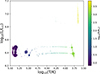 |
Fig. A.1. Temperature-luminosity diagram for the fiducial selected models as described in Section 2. The size of the points corresponds to the model weighting, and the colour to the final radius of the star. Most of the progenitors are WR stars or blue supergiants, with a smaller contribution from red supergiants (including those above the pair-instability mass gap). |
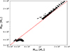 |
Fig. A.2. Carbon-oxygen core masses versus the final remnant mass, for the fiducial selected models as described in Section 2. The dashed red 1:1 line is a reasonable approximation of the Fryer et al. (2012) remnant mass prescriptions above ∼10 M⊙ (see also Briel et al. 2023). The BPASS remnant masses deviate from this by no more than 10–20% level below the pair instability mass gap and track it above. |
Appendix B: Disc radii
To calculate the initial disc radii - for input to the model of Mummery & Balbus (2020), Mummery & van Velzen (2025) - we first define M★ = MBH + Mleftover. The initial disc radius can be estimated from angular momentum and mass conservation as the star is ‘turned’ (from a process that is not detailed in this work) into a Keplerian flow. Therefore, we need an estimate of the maximum angular momentum available to the disc. On the grounds of energetics, for the pre-collapse star, we can assume
 (B.1)
(B.1)
where vcrit is the maximum pre-collapse stellar rotational velocity. The corresponding specific angular momentum of the star jcrit is approximately ∼R★vcrit. Substituting into equation B.1 (and ignoring constants of order unity) we find
 (B.2)
(B.2)
therefore, we have
 (B.3)
(B.3)
The angular momentum in the accretion disc has to be less than or equal to the total pre-collapse angular momentum; therefore,
 (B.4)
(B.4)
Where  and r0 is the initial disc radius. We therefore find an absolute maximum2 initial disc radius of
 (B.5)
(B.5)
in the extreme case that (i) the star is maximally rotating and (ii) the total pre-collapse angular momentum is transferred entirely to the disc. Since jcrit ∝ vcrit and  we can introduce factors to allow for sub-critical rotation velocities v★, and the fraction of angular momentum which goes into the disc fj, disc, as follows:
 (B.6)
(B.6)
Finally, we adopt 0.1vcrit for the pre-collapse rotational velocity and introduce the fraction of leftover mass which is accreted facc, yielding
 (B.7)
(B.7)
as adopted in Section 4.3.
The disc then must expand, as angular momentum is conserved while the mass of the flow drops (as some material is added to the BH). To be precise, the quantity
 (B.8)
(B.8)
is conserved. The mass in the disc drops with time in a self similar fashion, as the accretion rate is
 (B.9)
(B.9)
at large times (e.g. Pringle 1981), such that
 (B.10)
and, thus,
 (B.11)
Of course, this expansion of the disc can be suppressed if angular momentum is lost from the discl namely, if angular momentum is transported to large radii by winds. It is important therefore that the radii at large times (in this model) are larger than that inferred from observations.
All Tables
All Figures
|
Fig. 1. Mean ratio of the rate of BH formation above a minimum mass, MBH, min, to the rate of CC SNe at z < 0.4. The black line shows this ratio as a function of MBH, min assuming the metallicity-dependence cosmic star-formation history (CSFH) of Langer & Norman (2006). The red and blue lines, bounding the grey shaded region, are the result of adopting a CSFH shifted up/down by 0.2 dex in 12+log(O/H), respectively. The horizontal dashed line is the estimated LFBOT volumetric rate (Ho et al. 2023b). We therefore find that the predicted formation rate of BHs with masses greater than (38 |
| In the text | |
|
Fig. 2. Cumulative distribution of LFBOT host galaxy metallicities is shown in orange (see Table 1). We sample the Z values, assuming Gaussian uncertainties, 100 times, producing the many realisations of the cumulative distribution shown. Cumulative distributions of our selected progenitor metallicities, weighted by the CSFH(Z) at z < 0.4, are also shown. The black line is the z < 0.4 mean metallicity distribution of star-forming galaxies Langer & Norman (2006). The grey shaded region bounded by dashed lines is defined by shifting the distribution of Langer & Norman (2006) by ±0.2 in 12+log10(OH), covering the high- and low-Z extremes defined by Chruslinska & Nelemans (2019). |
| In the text | |
|
Fig. 3. Leftover (i.e. ejected and/or accreted) mass fractions of hydrogen (Xsurf) and helium (Ysurf) in the last time-step of the selected BPASS models, with contributions from different metallicities determined by the mean metallicity spread at z < 0.4 (Langer & Norman 2006). The colourbar indicates the number of events per 106 M⊙ of star formation, with contributions from different metallicities following the fiducial case as shown in Figure 2, along with the model weightings as defined in Section 2. |
| In the text | |
|
Fig. 4. Remnant BH mass versus the ‘leftover’ mass for the models selected when the fiducial CSFH is used (black lines in Figures 1 and 2). These are the remnant and leftover (ejecta) masses when an CC energy injection of 1051 erg is assumed (Eldridge & Tout 2004), taking into account the mass gap from PISNe and PPISNe (Farmer et al. 2019; Briel et al. 2023). The histograms show the number events expected per 106 M⊙ of star formation, as described in Figure 3. |
| In the text | |
|
Fig. 5. Wind density parameter for the selected models, normalised by a typical WR mass-loss rate and wind speed. The circumstellar densities resulting from these values are lower than typical WR stars and lower than observed in some LFBOTs, likely due to weaker winds as a result of the strong low-metallicity bias introduced by requiring such massive BHs. Typical LFBOT values are in the range 1–100 (e.g. Ho et al. 2022; Bright et al. 2022). The y-axis indicates the number events per 106 M⊙ of star formation, as described in Figure 3. |
| In the text | |
|
Fig. 6. Left: Predictions for UV light curves arising from the accretion disc around natal BHs of mass greater than 38 M⊙ in our failed SN models, using the model of Mummery & Balbus (2020), Mummery et al. (2025). These predictions are for observations in the Hubble Space Telescope WFC3/F225W filter; the black points are late-time F225W observations of AT 2018cow (Inkenhaag et al. 2023). Two example cases are shown: one assuming that 10% of the total pre-collapse angular momentum and 10% of the leftover mass, goes into the disc (red). The other is the extreme case that 100% of the available angular momentum and mass goes into the disc (cyan). Both scenarios adopt progenitor rotation at 10% of the critical velocity. The large spread in luminosity in both the cyan and red curves is due to the spread in BH and leftover masses (spanning the pair instability mass gap, see Figure 4). Right: Disc radii for the fiducial selected models at t = 0, 1, and 1000 days. The radii are the same for both the 10% and 100% assumptions (see Equation 1). The discs spread rapidly, with around 40% of them reaching radii of 30–40 R⊙ within the first day (the scale inferred from blackbody modelling of LFBOT observations). All discs ultimately reach 100–1000 R⊙ by 1000 days. |
| In the text | |
|
Fig. A.1. Temperature-luminosity diagram for the fiducial selected models as described in Section 2. The size of the points corresponds to the model weighting, and the colour to the final radius of the star. Most of the progenitors are WR stars or blue supergiants, with a smaller contribution from red supergiants (including those above the pair-instability mass gap). |
| In the text | |
|
Fig. A.2. Carbon-oxygen core masses versus the final remnant mass, for the fiducial selected models as described in Section 2. The dashed red 1:1 line is a reasonable approximation of the Fryer et al. (2012) remnant mass prescriptions above ∼10 M⊙ (see also Briel et al. 2023). The BPASS remnant masses deviate from this by no more than 10–20% level below the pair instability mass gap and track it above. |
| In the text | |
Current usage metrics show cumulative count of Article Views (full-text article views including HTML views, PDF and ePub downloads, according to the available data) and Abstracts Views on Vision4Press platform.
Data correspond to usage on the plateform after 2015. The current usage metrics is available 48-96 hours after online publication and is updated daily on week days.
Initial download of the metrics may take a while.