| Issue |
A&A
Volume 706, February 2026
|
|
|---|---|---|
| Article Number | A255 | |
| Number of page(s) | 12 | |
| Section | Extragalactic astronomy | |
| DOI | https://doi.org/10.1051/0004-6361/202557710 | |
| Published online | 17 February 2026 | |
Delving into the depths of NGC 3783 with XRISM
IV. Mapping of the accretion flow with Fe Kα emission lines
1
Leiden Observatory, Leiden University PO Box 9513 2300 RA Leiden, The Netherlands
2
SRON Netherlands Institute for Space Research Niels Bohrweg 4 2333 CA Leiden, The Netherlands
3
Space Telescope Science Institute 3700 San Martin Drive Baltimore MD 21218, USA
4
Lawrence Livermore National Laboratory Livermore CA 94550, USA
5
ESA European Space Research and Technology Centre (ESTEC) Keplerlaan 1 2201 AZ Noordwijk, The Netherlands
6
MIT Kavli Institute for Astrophysics and Space Research, Massachusetts Institute of Technology Cambridge MA 02139, USA
7
Center for Astrophysics | Harvard & Smithsonian 60 Garden St. Cambridge MA 02138, USA
8
Science Research Education Unit, University of Teacher Education Fukuoka, Munakata Fukuoka 811-4192, Japan
9
Department of Astronomy, University of Michigan Ann Arbor MI 48109, USA
10
Department of Physics and Astronomy, James Madison University Harrisonburg VA 22807, USA
11
Department of Physics, Technion Haifa 32000, Israel
12
INAF – Osservatorio Astrofisico di Arcetri Largo Enrico Fermi 5 I-50125 Florence, Italy
13
University of Maryland College Park, Department of Astronomy College Park MD 20742, USA
14
NASA Goddard Space Flight Center (GSFC) Greenbelt MD 20771, USA
15
Center for Research and Exploration in Space Science and Technology, NASA GSFC (CRESST II) Greenbelt MD 20771, USA
16
ESA European Space Astronomy Centre (ESAC) Camino Bajo del Castillo s/n 28692 Villanueva de la Cañada Madrid, Spain
17
Institute of Space and Astronautical Science (ISAS), Japan Aerospace Exploration Agency (JAXA) Kanagawa 252-5210, Japan
18
Graduate School of Science and Engineering, Kagoshima University Kagoshima 890-8580, Japan
19
Department of Astronomy, Kyoto University Kitashirakawa-Oiwake-Cho Sakyo Kyoto 606-8502 Kinki, Japan
★ Corresponding author: This email address is being protected from spambots. You need JavaScript enabled to view it.
Received:
15
October
2025
Accepted:
8
December
2025
Abstract
Using XRISM/Resolve 439 ks time-averaged spectra of the well-known Seyfert-1.5 active galactic nucleus (AGN) in NGC 3783, we investigated the nature of the Fe Kα emission line at 6.4 keV, the strongest and most common X-ray line observed in AGNs. Even the narrow component of the line is resolved with evident Fe Kα1 (6.404 keV) and Kα2 (6.391 keV) contributions with a 2:1 flux ratio, fully consistent with a neutral gas with negligible bulk velocity. The narrow and intermediate-width components have a full width at half maximum of 350 ± 50 km/s and 3510 ± 470 km/s, respectively, suggesting that they arise in the outer disk/torus and/or broad line region. We detect a 10% excess flux around 4–7 keV that is not described well by a symmetric Gaussian line but is consistent with a relativistically broadened emission line. In this study we took the simplest approach, modelling the asymmetric line as a single emission line (assuming neutral, He-like, or H-like iron) convolved with a relativistic disk line model. As expected, the inferred inclination angle (i) is highly sensitive to the assumed ionisation state and ranges between 17 and 44°. This model also constrains the black hole spin via the extent of the red wing: the required gravitational redshift in the fitted disk-line profile disfavours a non-spinning (Schwarzschild) black hole. The derived inner radius is close to the radius of the innermost stable circular orbit (rISCO) and is strongly correlated with the black hole spin. To better constrain the spin, we fixed the inner radius to rISCO and derived a lower limit on the spin of a ≥ 0.29 at the 3σ confidence level. A Compton shoulder is detected in our data as well as a 2–3σ detection of the Cr Kα and Ni Kα lines.
Key words: techniques: spectroscopic / galaxies: active / galaxies: Seyfert / X-rays: galaxies / X-rays: individuals: NGC 3783 Fe K band
© The Authors 2026
 Open Access article, published by EDP Sciences, under the terms of the Creative Commons Attribution License (https://creativecommons.org/licenses/by/4.0), which permits unrestricted use, distribution, and reproduction in any medium, provided the original work is properly cited.
This article is published in open access under the Subscribe to Open model. This email address is being protected from spambots. You need JavaScript enabled to view it. to support open access publication.
1. Introduction
The Fe Kα line, at a rest-frame energy of 6.4 keV, is a prominent emission feature in active galactic nucleus (AGN) spectra; it originates from X-ray fluorescence in dense material surrounding the supermassive black hole (SMBH). Its line width varies significantly, revealing the diverse physical processes taking place in different regions of the AGN environment (Gallo et al. 2023). Narrow Fe Kα lines of a few hundred or thousand km/s likely originate from distant, cold, and dense material such as the torus or outer disk. They provide insights into the structure and geometry of the circumnuclear environment (Reynolds et al. 1994; Yaqoob & Murphy 2011; Gandhi et al. 2015). In contrast, the broad Fe Kα lines, often very extended and skewed with widths of ten to a few hundred thousand km/s, arise from the innermost regions of the accretion disk, where gravitational redshift and relativistic effects significantly broaden and distort the line profile. The presence and characteristics of the broad Fe lines encode valuable information about the disk inner radius, the ionisation state, the influence of strong gravity, and the spin of the SMBH (Fabian et al. 1989, 1995; Laor 1991; Brenneman & Reynolds 2006).
With the existing X-ray instruments, isolating and characterising the broad relativistic Fe Kα line remains challenging: CCDs do not have enough spectral resolution and blend multiple lines, and grating spectra lack the effective area needed for adequate S/Ns. The measurement is critically dependent on several systematic effects, including the shape of the underlying continuum, the presence of ‘clumpy’ absorbers, and the presence of potential Fe lines with intermediate line widths from the optical/X-ray broad-line regions (BLRs). To overcome these challenges, high-resolution spectroscopy in the Fe Kα band coupled with simultaneous modelling of all the relevant spectral components, together with high-S/N data, are essential, especially in time-averaged spectra (Reynolds et al. 2012). Energy-dependent lag spectra can further be used to test whether the broadband variability around the Fe Kα band originates from clumpy absorption or is intrinsic to the central source (Zoghbi et al. 2019; Reis et al. 2012).
The recent launch of the X-Ray Imaging and Spectroscopy Mission (XRISM) marks a significant advancement in our ability to study these Fe lines (Tashiro et al. 2025). With its high spectral resolution, the Resolve instrument on board XRISM can distinctly separate emission and absorption components with varying widths (Ishisaki et al. 2025; Kelley et al. 2025). Early results demonstrate that what was previously thought to be a single narrow line is actually a complex blend of several components, each originating from different regions, such as the torus, the BLR, and the inner accretion disk (XRISM Collaboration 2024).
The Seyfert 1 galaxy NGC 3783 (z = 0.00973; Theureau et al. 1998) has been extensively examined for its X-ray wind components (Kaspi et al. 2002; Netzer et al. 2003; Mao et al. 2019; Gu et al. 2023). Due to its brightness in the Fe K band, it was selected as a XRISM performance verification target to probe the highly ionised gas resolved by velocity (Mehdipour et al. 2025). Furthermore, the full absorption measure distribution of the X-ray outflow will be determined by combining XRISM observations with XMM-Newton reflection grating spectrometer (RGS) observations (Zhao et al. 2025 in prep., Paper V). Simultaneously, it offers an unprecedented opportunity to investigate the nature of the Fe Kα emission line with the help of the resolved Fe K band absorption lines detected by Resolve, which is the main scientific goal of the present paper.
Using the combined data taken in 2000–2001 by the Chandra High Energy Transmission Grating Spectrometer (HETGS), the full width at half maximum (FWHM) of the narrow Fe Kα line core in NGC 3783 was determined to be approximately 1800 km/s; it is located between the BLR and the narrow-line region (Kaspi et al. 2002; Yaqoob et al. 2005). It was also found that the excess flux around the base of the narrow Fe Kα line core can be modelled with either a Compton-scattering ‘shoulder’ or a relativistic line from the inner disk with a low inclination angle of 11° or less. From the XMM-Newton EPIC data taken in 2001, Reeves et al. (2004) found not only a strong broader Fe Kα line at 6.4 keV but also another peak feature at 7.05 keV probably originating from a blend of the neutral Fe Kβ line and the hydrogen-like line of Fe at 6.97 keV. They also reported a weak, broad red wing, attributed either to an ionised warm absorber or to relativistic effects (Reeves et al. 2004).
Using a deep (210 ks) Suzaku observation from 2009, Brenneman et al. (2011) and Reis et al. (2012) reported a strongly broadened and skewed iron line and concluded that the black hole (BH) is rapidly spinning in the prograde direction. Patrick et al. (2011) obtained different results using the same dataset, finding a slowly or retrograde spinning BH with a ≤ −0.04. Motivated by this discrepancy, Reynolds et al. (2012) performed a Monte Carlo Markov chain-based investigation of BH spin in NGC 3783 and identified a (partial) modelling degeneracy between the iron abundance of the disk and the BH spin parameter. Moreover, the two different methods used by Capellupo et al. (2017), namely relativistic reflection and continuum fitting, yield a wide range for the spin parameter, albeit with a high probability of a near-maximal spin if a disk wind is included in the reflection model.
Using all the archival data collected by the Chandra/HETGS, Danehkar & Brandt (2025) determined that the relativistically broadened iron emission is consistently associated with a near-maximal BH spin across all analysed datasets. This high spin is a constant finding even when the system transitions to different spectral states, such as the hard state due to some transient obscuration events caused by eclipsing outflow material near the X-ray source (Mehdipour et al. 2017), which was present in data from 2013 to 2016. The analysis of HETGS data by Danehkar & Brandt (2025) also shows that the narrow Fe Kα line from distant regions has an excess redshift velocity of a few hundred km/s relative to the rest frame, suggesting that a warped disk scenario is causing the far side of the disk to be more illuminated.
With its unprecedented energy resolution and enhanced effective area in the Fe K band, the XRISM Resolve instrument is poised to advance our understanding of the Fe Kα complex in NGC 3783. This paper is organised as follows. Section 2 presents the spectral modelling method and analysis. Section 3 describes the narrow Fe Kα observational characters and the broad iron emission spectral modelling results. We summarise and discuss all of the results in Sect. 4.
2. Spectral modelling and analysis
NGC 3783 was observed by XRISM/Resolve during 10 days (ObsID 300050010) from July 18–27, 2024. We used the exact same spectral data as Paper I and XRISM Collaboration (2025); we refer readers to these works for comprehensive details on data reduction and analysis. For clarity, we highlight the related information in our current paper. Of the 36 pixels of Resolve instrument, pixel 12 (calibration pixel) and pixel 27 (which shows unpredictable gain jumps) were excluded from the analysis. Only high-resolution primary events (Ishisaki et al. 2018) were selected for our analysis. The count rate was approximately 0.1 s−1 pix−1 in the four central pixels and ranged from 0.001 to 0.1 s−1 pix−1 in the outer pixels. To mitigate contamination, all low-resolution secondary events were excluded before creating the extra-large response matrix file, which includes all known instrument effects.
The gain uncertainty is 0.16 eV at 5.9 keV and the systematic energy scale uncertainty is 0.3 eV in the band of 5.4–8.0 keV, which are uncorrelated and can be root-sum-squared. The total systematic uncertainty corresponds to 15 km s−1 at 7 keV. The FWHM of 5 eV at 6.4 keV is equivalent to 234 km/s at 6.4 keV. The non-X-ray background spectrum was modelled from the Resolve night-Earth data database1, while the sky background was ignored because its contribution above 2 keV is negligible.
We modelled the time-averaged 439 ks XRISM/Resolve spectrum (optimally binned to ≈2 eV with obin; see Kaastra & Bleeker 2016) using SPEX v3.08.01 (Kaastra et al. 1996, 2024) along with an atomic database SPEXACT version 2.07.00. Spectral fitting was performed with C-statistics (Kaastra 2017). The cosmological redshift was fixed at 0.009730 (Theureau et al. 1998). Galactic X-ray absorption was calculated using the hot model in SPEX, with a column density of NH = 9.59 × 1020 cm−2 (Murphy et al. 1996). The abundances of all components were set to the protosolar values of Lodders et al. (2009).
2.1. Modelling of the photo-absorption continuum
The time-averaged Resolve spectrum was modelled by a power-law component in the 4–10 keV band, excluding the 2–4 keV as well as the 5–8 keV ranges where multiple absorption line features are present (Kaspi et al. 2001). As shown in Fig. 1a, the model falls below the data, in particular towards 4 keV, suggesting the presence of an additional underlying component.
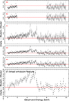 |
Fig. 1. XRISM/Resolve residual spectra for each added model component: power law (a); photo-absorbed power law (b); all data, with narrow absorption lines excluded as described in the text (c); narrow Fe core added (d); intermediate neutral Fe component added (e); and a residual broad emission feature, re-binned to 60 eV to better reveal the broad emission structure (f). |
Building on the models reported in Papers I and V, our second step was to incorporate warm absorber components to model in particular the continuum absorption. We applied five slab components to incorporate the impact of photo-absorption; their ion column densities are taken from Paper V. These five components in order correspond to components C1, A1, A3+B+C2, and A2 of Paper V, as described from a joint fit using pion components of the combined Resolve and RGS spectra. The pion model is a fully self-consistent model that computes the absorption and emission for a photoionised plasma (Mehdipour et al. 2016; Miller et al. 2015). The slab model is a pure empirical model for the transmission of a layer of material with arbitrary ionic column densities (Kaastra et al. 2002). To maintain physical consistency, we adopted the ionic column densities obtained from their pion fits as inputs to slab in our current work, ensuring that the absorption continuum is treated in a physically consistent manner and reduces computational cost.
The transmission of these components is plotted in Fig. 2 for reference. We only retained the total continuum absorption (black curve in Fig. 2) caused by these warm absorbers when we modelled the continuum using the broadband data of 4–5 keV and 8–10 keV. Including the weak lines in these bands has a negligible effect on the derived power-law parameters. Figure 1b illustrates the improvement in the model by incorporating this continuum absorption. We did not incorporate the component X, the fast (v ∼ 14 300 km/s) outflowing wind component in Paper I, as this component only has 1%–2% effect on the continuum seen from the transmission. We have not included the Compton hump in our continuum model. Based on the work of Mao et al. (2019), its contribution is negligible at 10 keV (typically less than 1%) and is even smaller at lower energies.
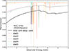 |
Fig. 2. Transmission of five warm absorber components determined using the slab model with Resolve data. In this emission-line and continuum modelling, we include only the total continuum absorption from the warm absorbers (shown in black). |
To minimise systematic uncertainties in modelling Fe-K emission components, we excluded all spectral bins from the spectral analysis, which contained significant absorption lines in the 6.38–7.1 keV range (see Fig. 1 of Paper I). Figure 1c shows the residuals of the full spectrum (excluding the absorption line data discussed above) to the continuum model described in this section. And the full spectrum was applied to the following data analysis.
2.2. Narrow and intermediate-width Fe K emission modelling
The neutral Fe Kα emission is not a single emission line, but a line complex composed of emission from numerous atomic transitions. An accurate model of the natural line shape of the Fe Kα complex must be incorporated when the velocity broadening is less than ∼2000 km/s (Yaqoob 2024). Here, we adopted the line profile of the seven-Lorentzian decomposition derived from high-precision laboratory measurements reported by Hölzer et al. (1997). For Fe Kα, the profile provided by Hölzer et al. (1997) is dominated by two strong complex, Fe Kα1 (6.404 keV) and Fe Kα2 (6.391 keV), separated by about 13 eV. This split of Fe Kα1 and Fe Kα2 peaks is seen in the time-averaged Resolve spectrum of NGC 3783. We adopted the Fe Kβ line profile from the same laboratory measurement, scaling the flux ratio between Fe Kα and Fe Kβ to 8:1, which is the characteristic ratio for neutral Fe fluorescence (Yamaguchi et al. 2014). Finally, we combined them into a file model in SPEX, which includes Fe Kα1, Fe Kα2, and Fe Kβ lines convolved with the same velocity broadening and redshift for representing the cold neutral line.
Similarly to the case of NGC 4151, the apparently narrow peak of the Fe Kα line complex may contain different velocity broadening components (XRISM Collaboration 2024). To investigate this, we employed a multiple component model. Each component consisted of a fixed intrinsic line profile as described above, which was convolved with a Gaussian broadening and shifted by a free velocity. Two components are found to be sufficient to reproduce the observed narrow Fe emission feature. Figure 1d shows the remaining residuals after inclusion of a narrow emission core with a few hundred km/s. Figure 1e shows the residuals after including the second intermediate width component of a few thousand km/s.
2.3. Broad emission feature between 4 and 7 keV
After modelling the continuum and the narrow emission lines, a broad, skewed residual remains, reaching ∼10% above the model between 4 and 7 keV (Fig. 1e). In Fig. 1f we re-bin this asymmetric structure to 60 eV bins to better highlight the broad emission. Such a broad emission feature can potentially arise from a relativistically broadened iron line of the inner accretion disk. Under this assumption, we fitted the structure using the unbinned high resolution spectrum (∼2 eV) assuming an intrinsically narrow iron line convolved with a relativistic line broadening model, spei in SPEX (Speith et al. 1995). This kernel is designed to handle a variety of BH spins, inclination angles of disk, and complicated emissivity profiles, as well as different regions of the disk. We used a delt line model convolved with spei to model the broad emission feature. For the delt component, the normalisation parameter is free and the energy of the line is kept frozen at a specified value. For the spei component, we allowed the inner radius of the disk (rin), BH spin (a), inclination angle (i), and emissivity slope (q) to vary freely during the fit. We fixed the emissivity scale height parameter (h) in the spei model to zero, which corresponds to a pure power-law emissivity profile2. Although a common empirical approach is to fix the inner radius (rin) to risco, the theoretical innermost stable circular orbit (ISCO), which depends on the spin, here we permitted the inner radius to extend beyond the ISCO to investigate the possibility of disk truncation outside the ISCO.
The broad iron line originates from reflection off the inner regions of the accretion disk. The dominant iron ion species contributing to this feature depend on the ionisation state of the disk surface. To explore different ionisation states of the inner disk, we investigated limiting cases where the intrinsic lines are either neutral or highly ionised. For the neutral line scenario, Model A, we included two delta line components with fixed energies, one for Fe Kα at 6.4 keV and another for Fe Kβ at 7.05 keV, coupling the normalisation of Fe Kβ to Fe Kα and keeping the flux ratio between Fe Kα and Fe Kβ 8:1, both were convolved by the same spei model. For the highly ionised disk cases, we explored the He-like Model B and H-like Model C ionisation conditions. In these scenarios, we used the delt model and fixed the line centres at 6.7 keV and 6.97 keV, respectively, convolved by the corresponding spei model. For all models the line flux is a free parameter. Adding the broad component to the fit Models A, B, and C, it improves the fit C-statistic by 1044, 1038, and 1033, respectively.
2.4. Compton shoulder modelling in 6.15–6.30 keV
The above components adequately describe the observed Resolve spectrum, with only a potential excess remaining between 6.0 and 6.4 keV (Fig. 3). Although the excess has a significance of only 2.1–2.4σ, the tail-like spectral feature could be generated via Compton scattering of neutral matter, known as a Compton shoulder (CS; Odaka et al. 2016). We modelled this feature with the file model for neutral intrinsic Fe Kα and Fe Kβ profiles of the emission line (see Sect. 2) convolved with the vcom model. The vcom model is a phenomenological model for single Compton scattering, with an option for an empirical skewness correction (a) such that the profile is proportional to (1+y2)(1+ay) with y the scaled energy between −1 and 1. In the vcom model, we kept the skewness parameter (a) thawed to fit the data. Including the CS model improves the C-stat value by 12, 9, and 9, respectively, for Models A, B, and C.
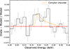 |
Fig. 3. XRISM/Resolve residual plot of NGC 3783 after modelling the Fe Kα core with three emission components. The residuals are modelled with the yellow line in Fig. 4. |
2.5. Neutral Cr Kα and Ni Kα
There are still a few line-like excesses at the Cr Kα (5.36 keV) and Ni Kα (7.40 keV) energies. Similarly to Fe, the Cr Kα and Ni Kα lines are modelled using natural line shapes provided by Hölzer et al. (1997), and convolved with a Gaussian broadening profile (vgau). We forced the broadening of these two lines to be equal to that of the narrow Fe Kα component. The Cr Kα component improves the C-stat by 8, 7, and 12 for Models A, B, and C, respectively. The Ni Kα component improves the C-stat by 11, 15, and 15 for Models A, B, and C, respectively.
2.6. Other ionised emission lines
The 6.8–7.1 keV band of Resolve is complex with possible contributions of neutral Fe Kβ and Fe XXVI Lyα absorption and emission, the Fe I K absorption edge, and the relativistic iron line blue edge. The weak Fe XXVI emission line has less than a 2σ significance after modelling. Due to its weakness and the complexity of this narrow energy band, we refrained from a more detailed analysis. In addition to weak Fe XXVI emission lines, other weak relative low ionised iron emission lines in the 6.4–6.6 keV band could possibly be present. We did not investigate them further because they are not significant in our current data.
3. Results
The Resolve spectrum reveals narrow Fe Kα and Kβ lines, alongside a series of absorption lines from highly ionised warm absorbers. A broad emission structure with a 10% excess above the continuum was clearly detected and is presented in the bottom panel of Fig. 1. Figure 4 illustrates one of the best-fit models, Model A, along with the profiles of its individual components. Model A provides acceptable fits to the Resolve data, with a C-statistic of approximately 2046, compared to an expected value of 2013 ± 64. Additionally, the broad emission feature can be reproduced well by a relativistic Fe line component. We examined three different models to fit this feature, as described in Sect. 2.3. All these solutions yield profiles that are similar to each other, and the resulting best-fits of the three models (Models A, B, and C) are generally in agreement. Figure 5 compares the three models with the data. While they generally agree, a modest discrepancy appears in the narrow Fe Kβ feature near ∼7 keV, which is attributable to relativistic Fe Kβ emission added in Model A. Figure 6 presents the relativistic iron line profiles corresponding to the best-fits of the different models, showing that the profiles (red, blue, and green curves) differ only slightly. Table A.1 presents the best-fitting parameters with 1σ errors and C-statistic values for Models A, B, and C.
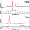 |
Fig. 4. XRISM/Resolve time-averaged spectrum of NGC 3783 with the best-fitting model shown as a solid red line. Top two panels: Resolve background-subtracted spectrum with individual model components and the corresponding fit residuals. The fit residuals are defined as (data − model)/model. In our fitting, we used all data points in black and excluded the strong absorption line data points (in grey) when the modelling continuum and emission lines independently. For visualisation purposes, the spectrum in the top panel is additionally binned up to 8 eV. Bottom two panels: Close-up view of the Fe K band and its fit residuals at the model optimal bin size of 2 eV. In both panels, the strongest emission features are labelled. The individual components are plotted with dashed lines representing the power law (cyan), the narrowest (magenta) and intermediate (purple) iron components, the relativistic iron line (blue), the CS (orange), and Cr Kα and Ni Kα (green). The background model is depicted by the grey curve. |
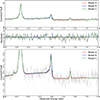 |
Fig. 5. XRISM/Resolve spectra of NGC 3783 fitted with three different models: Model A (red), Model B (blue), and Model C (green). The top two panels illustrate the subtle differences between these models. Residuals are calculated as (data − model)/model, as in Fig. 4. The bottom panel shows a close-up view of the complex spectral structure in the 6.75–7.1 keV energy range. Spectral bins containing narrow absorption features are included in the spectral plot but excluded from the residual plot. |
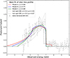 |
Fig. 6. Modelling relativistic iron line profiles. The red, blue, and green curves represent the best-fit relativistic iron line profiles of Models A, B, and C, respectively. The dotted and dashed grey lines are non-spin BH solutions with different emissivity slopes. The former is derived from a grid search based on Table A.2, and the latter is one of solutions shown in Fig. 9. Both profiles correspond to the minimum C-statistic value for a non-spinning BH case. The grey data points represent the residuals of Model A (data − model) excluding the relativistic iron line, binned to 60 eV. |
When we performed error analysis, we found several strong correlations between the parameters of the Speith profile. To investigate this, we performed a grid search to examine the degeneracy of spei model parameters using the step command in SPEX. The step sizes and parameter ranges are shown in Table A.2. The normalisation of the line is always adjusted to the best-fit value for the given parameter set. The results of this grid search are shown in Fig. 7, which presents the degeneracy between rin/risco and spin. Following Fig. 7, Fig. 8 shows the inner radius versus BH spin, illustrating the uncertainty in the inner radius for our current modelling.
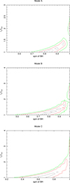 |
Fig. 7. Contour plot of the ratio of the inner radius to the ISCO (rin/risco) and the spin of the BH with the Resolve time-averaged spectrum of NGC 3783. The same parameter space is applied for the grid search of Models A, B, and C. The 1σ (68%), 2σ (95%), and 3σ (99.7%) confidence contours are in black, red, and light green, respectively. |
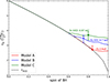 |
Fig. 8. Best-fit inner radius as a function of spin (coloured lines). For each model, the best-fit inner radius is shown as a filled circle, together with the associated 1σ uncertainty from Table A.1. The prograde ISCO radius as a function of spin is shown as the dashed black line. |
To better constrain the spin, we fixed the inner radius to the ISCO at each spin value (rin = rISCO) and allowed the emissivity index and inclination to vary freely (no grid limits). The resulting distribution of C-statistic values is shown in Fig. 9; the best-fitting spin and its 3σ error bar are indicated, disfavouring a non-rotating BH.
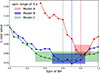 |
Fig. 9. Distribution of C-statistic values as a function of spin, with the inner radius fixed to the ISCO at each spin (rin = rISCO). For each model, the best-fitting spin is indicated by a vertical line. We show the 3σ confidence interval on the spin (shaded coloured region), which clearly demonstrates that a non-spinning BH solution is ruled out. |
4. Discussion
The 439 ks time-averaged spectrum of NGC 3783, taken by XRISM/Resolve in July 2024, has shown rich results. The Fe Kα emission complex is clearly resolved into three components: a narrow feature with a FWHM of ∼300 km/s, an intermediate-width component with a FWHM of ∼3500 km/s, and a broadest emission structure spanning 4–7 keV. Their respective equivalent widths are EWnar = 48 ± 3 eV, EWintm = 48 ± 4 eV, and EWbrd = 278 ± 14 eV. The narrow Fe Kα is accompanied by a weak and moderately broadened CS. Additional weak emission lines, including Cr Kα and Ni Kα, were detected at a significance level of approximately ∼3 − 4σ, with Gaussian velocity widths comparable to the Fe Kαnar component.
4.1. Narrow iron Kα lines
The detection of the narrow Fe Kα line component helps us better interpret the distant reflection regions in NGC 3783. The fluorescence line properties can potentially be used to constrain the geometry, column density, and kinematics of the material in which the line is formed (Murphy & Yaqoob 2009; Yaqoob & Murphy 2011; Yaqoob 2024; Vander Meulen et al. 2024). The spectrum shows a clear split of Fe Kα1 and Fe Kα2, which is consistent with the neutral Fe Kα profile.
The FWHM of the Fe Kα core of 1720 ± 360 km s−1 measured by the Chandra grating data from 2001 (Kaspi et al. 2002), lies between the narrow (FWHM = 350 ± 50 km/s) and intermediate (FWHM = 3510 ± 470 km/s) components in our analysis. Fitting the Resolve spectrum with a single Fe Kα core component by delt*vgau yields a FWHM of ∼1390 ± 40 km/s, consistent with the Chandra value. The Chandra/HETGS spectral resolution is worse than that of XRISM/Resolve at these energies by at least a factor of ∼6. This suggests that the profile of the Fe core has remained stable over a timescale of approximately 24 years.
If we assume virial motion for the emitting clouds producing the narrow and intermediate velocity component, we have
 (1)
(1)
where MBH is the BH mass, v is the de-projected orbital velocity. Following Gandhi et al. (2015), we related v to the observed line width and the line-of-sight inclination (i) as
 (2)
(2)
where vFWHM = 2.35σv, the σv is the Gaussian width of the line. Equations (1) and (2) imply
 (3)
(3)
Applying Eq. (3), we adopted i ≈ 23 degree (GRAVITY Collaboration 2021b), and  for NGC 3783, which was estimated based upon a joint analysis that combines both GRAVITY and optical reverberation mapping data (GRAVITY Collaboration 2021a) to estimate the distance of Fe Kα complex.
The narrow component is likely located at ∼5 × 10⁵ Rg, corresponding to ∼0.64 pc with a typical ∼30% uncertainty. This is a factor of ∼4–5 beyond the hot-dust radius (∼0.14 pc) measured with near-IR interferometry (GRAVITY Collaboration 2021b), in contrast to Gandhi et al. (2015), who inferred an origin inside the hot-dust region from Chandra/HETGS data. Given rFe ∝ sin2(i) dependence, the estimated rFe is sensitive to the line-of-sight inclination. Accounting for the uncertainty in i, the inferred rFe remains broadly consistent with the results of Gandhi et al. (2015). Moreover, geometry can further bias the effective viewing angle: if our sight-line is dominated by the illuminated inner face of the torus/BLR, the effective inclination is smaller with big opening angle.
The intermediate Fe core component is likely emitted from a radius of ∼5 × 10³ Rg (∼0.006 pc or 7.6 light-days), which falls within the BLR (∼3–20 light-days) reported from optical spectroscopy by Bentz et al. (2021a) and Bentz et al. (2021b). In their work, the inferred kinematics of the outer BLR as probed by Hβ are dominated by near-circular orbits with a contribution from infall, whereas the kinematics of the inner BLR probed by He II is dominated by an unbound outflow. The difference in kinematics between the Hβ- and He II-emitting regions of the BLR is intriguing given the large changes in the ionising luminosity of NGC 3783 during an obscured state (Mehdipour et al. 2017) and evidence of possible changes in the BLR structure as a result. A caveat in comparing the XRISM/Resolve measurements with BLR sizes from earlier optical campaigns is the source state: those optical data were taken when NGC 3783 was obscured, whereas our 2024 XRISM observations captured it in an unobscured state. A coordinated XRISM campaign with simultaneous optical spectroscopy would be the most robust way to test whether the intermediate Fe Kα core is physically connected to the BLR.
In Table A.1, the centroids of the Fe Kα complex for the narrow and intermediate widths were found to be within 10 and 300 km/s redshift from their rest frame energy, respectively. These line centroids are within the systematic uncertainty of the Resolve instrument. Previously, an excess redshift velocity of  km/s of the iron Kα line with respect to the host galaxy was found in NGC 3783 using Chandra ACIS-S/HETGS (Danehkar & Brandt 2025), which implies more redward photons were observed in the far side of the disk, potentially caused by a warped disk (Miller et al. 2018). The BLR in NGC 3783 can be accurately characterised as a thick, rotating disk with the highest cloud concentration in the inner region by GRAVITY Collaboration (2021b). The excess redshift of the Fe Kα emission found by Danehkar & Brandt (2025) could stem from a transient event, such as X-ray-emitting BLR inflow towards the SMBH, or a failed wind falling back towards the inner region (Mehdipour et al. 2017; Li et al. 2025).
Recent XRISM spectroscopic observations of NGC 4151 also suggest contributions from the innermost BLR (optical/X-ray) to the Fe Kα line, in addition to a potentially warped accretion disk (XRISM Collaboration 2024). Alternatively, as proposed by Miller et al. (2018), a failed wind could also result in an asymmetric narrow Fe Kα line.
4.2. Chromium and nickel lines
In addition to Fe, Cr Kα and Ni Kα lines are detected with significances of 2.8σ and 3–4σ, respectively. The observed line broadening is consistent with the velocity dispersion of the narrow Fe core. If we assume that the line flux for element Z scales as ∼IzωzAz, where Iz is the K-shell photoionisation rate (ionisation/ion), ωz is the fluorescence yield and Az is the abundance relative to hydrogen, we can estimate the expected line fluxes for Cr and Ni by scaling these parameters to the observed Fe flux. This yields predicted fluxes of 1.3 × 1047 photons s−1 for Cr and 4.0 × 1047 photons s−1 for Ni, which are in broad agreement with the observed values of 3.3 ± 1.2 and 3.4 ± 1.1 × 1047 photons s−1. The lines are therefore consistent with solar abundance ratios, although Cr might also be slightly enhanced. We need better data, for example a larger effective area (gate valve open) or a longer exposure time with Resolve, to perform accurate abundance measurement.
4.3. The Compton shoulder of Fe Kαnar
The potential CS of the Fe Kα core is marginally detected at approximately 2.4σ confidence. Its shape remains largely unconstrained (see Fig. 3), and its flux is estimated to be no more than 10% of the narrow Fe Kα line. This indicates an optical depth τ = 0.1, corresponding to a column density of matter emitting the CS of ∼1023 m−2 associated with scattering material. The luminosity of the narrow component of Fe Kα is close to that of the intermediate one (see Table A.1). Modelling shows that we cannot distinguish between the narrow and intermediate component as the source of the scattered photons. In contrast to the results reported by Yaqoob et al. (2005), where the broad Fe line and CS scenarios were degenerate in the Chandra data, our XRISM observations now allow us to clearly distinguish between them.
4.4. Relativistic reflection emission
One of the derived parameter from our model is the inclination angle of the accretion disk. A known degeneracy exists between the inclination, which is primarily determined by the blue edge of the relativistic line profile, and the intrinsic energy of the line. This is seen in Table A.1, where the inclination angle is found to decrease from ∼44°, to ∼32°, to ∼17° with increasing ionisation state (neutral iron, FeXXV, and Fe XXVI, respectively). The emissivity slope of the disk is found to be in the range 3–4. No clear correlation is found between this slope and other parameters, such as the ionisation state and the inclination angle.
The inner disk radius is a free parameter in our analysis. As shown in Fig. 7, this approach reveals a degeneracy between the ratio of the inner radius to ISCO and the BH spin: as the spin increases, the inner radius moves away from the ISCO. The black 1σ contour in Fig. 7 indicates that different spin solutions are possible in the disk line model. Based on Table A.2, our grid search also rules out non-spinning solutions with at least 3σ significance. The observed spectrum can be fitted equally well by two scenarios: a high-spin BH with a potentially truncated disk, or a mildly spinning BH with a disk extending to the ISCO inner radius.
Following up of Fig. 7, we examined the potential relationship between the absolute value of the inner radius and the BH spin. As shown in Fig. 8, while the ISCO radius decreases sharply with increasing spin (black dash line), the observed inner radius exhibits only minor variation for different spin values. The best-fit inner radius for the neutral line model is approximately 2.5–3 Rg. This value increases to 3–3.5 Rg for the ionised line in Model B and then slightly increases to 3.5–4 Rg for Model C. Since the observed profile likely blends emission from neutral, He-like, and H-like iron, we fitted each ionisation state separately and found a consistent result: the best-fit inner radius is rin ≈ 2.5–4 Rg in all cases where best-fit spins a > 0.6 correspond to rISCO < 4 Rg (the rISCO is strongly dependent on spin).
We next focused on the scenario that the disk is not truncated but extends to the ISCO radius. This possibility is not excluded from our analysis. To get proper constraints on the spin, we re-fitted data by fixing rin = rISCO for each spin, as described in Sect. 3. The C-statistic value versus spin is plotted in Fig. 9. The fitting results indicate that the allowed spin range for Models A, B, and C are 0.73 ≤ a ≤ 0.91, 0.48 ≤ a ≤ 0.85, and 0.29 ≤ a ≤ 0.998 with 3σ confidence level, respectively. Additionally, a non-spinning BH case leads to a significantly worse fit, with the C-stat increasing by 168, 70 and 42 for Models A, B, and C, respectively. These results indicate that a non-spinning solution is ruled out. The non-spinning BH model profile for Model A is shown as a dotted line in Fig. 6.
We further examined the case of a non-spinning BH with a high emissivity slope. We fixed a = 0 for Model A, while varying q from 2.0 to 6.0. The new best-fit yields a C-statistic value of 2187, which is worse than the best fit value of Model A. This indicates an emissivity slope of  and an inclination of
  degrees for the disk profile (see the dashed grey line in Fig. 6). This result also rules out the non-spinning BH scenario with a high emissivity slope based on the C-statistic value.
4.5. Comparison with previous studies and systematic uncertainty
Our derived inclination angle of 17.6 ± 1.4 degrees from Model C is slightly lower than the previous values: 19–22 degrees (Brenneman et al. 2011) and 22–24 degree (Reynolds et al. 2012). A rotating BLR model fitted to the VLTI/GRAVITY observations of NGC 3783 implies an inclination angle of the disk of either  degrees (GRAVITY Collaboration 2021b) or 32 ± 4 degrees when combined with a reverberation mapping analysis (GRAVITY Collaboration 2021a). This is in agreement with the confidence limits of our values obtained for the inclination angle of the accretion disk by Model B (32 ± 2 degree).
As shown in Table A.1, the emissivity slope q falls within the range of 3–4 across the three models. This result aligns with the standard emissivity profile expected in flat space-time. It differs from the steeper profiles (q ∼ 5 − 6) observed in some AGNs (such as MCG−6-30-15; Fabian & Vaughan 2003) due to strong GR light blending depending on the location/geometry of an illuminating source above the disk (Fukumura & Kazanas 2007; Dauser et al. 2013; Wilkins & Fabian 2012).
All of our best-fit models prefer spinning BH solutions as seen in Figs. 7 and 8. Our derived lower limit for the spin is a ≥ 0.29 at the 3σ significance level as seen in Fig. 9. It is consistent with values reported by Brenneman et al. (2011, a ≥ 0.88 with 99% confidence), Reynolds et al. (2012, a rapidly spinning BH a > 0.89), and Danehkar & Brandt (2025, a near-maximal SMBH spin  ). The large uncertainty on spin measurement in our analysis compared to other results can be due to many causes.
The measured spin here should be viewed as an initial constraint, with a more thorough analysis to be performed that includes the entire reflection spectrum rather than just the Fe Kα line. The latter approach will help eliminate many of the model degeneracies found in this paper (e.g. the ionisation state of the disk and the energy of the line, which impacts the measurement of the blue wing and inclination).
Excluding the absorption-line data points between 6.38 and 7.1 keV has no impact on our current final results. In principle, many factors affect the modelling of the relativistic iron line component. This includes the accounting for the intermediate-width Fe Kαβ component, inclusion of a relativistic Fe Kβ component, the absorption trough modelling of the Fe XXVI line, and the modelling of the remaining Fe XXVI emission line. This is hard or impossible to do with CCD spectra or grating spectra with relatively low sensitivity. While the Resolve instrument offers the spectral resolving power needed to precisely characterise the narrow emission and absorption features in the Fe-K region, it does not provide the same level of data statistics as the current CCD instruments utilised in several previous studies for the broad relativistic iron line component. A joint analysis incorporating the Xtend data would be ideal to further improve the constraints on the BH spin parameter.
A second difference between previous work and ours is that we used a single emission line while others used a full reflection model such as relxill (Dauser et al. 2016) to characterise the emission. Although such reflection models are dominated by one strong spectral line for a given ionisation state of the accretion disk in the 4–10 keV band of the Resolve spectrum, a self-consistency reflection model combining with soft and hard X-ray data will further improve spin measurement.
Finally, the spin measurement may be biased if the relativistic line shows strong variability. Time variability is the subject of follow-up papers, but a simplified preliminary analysis shows that apart from a strong soft flare (Gu et al. 2025), the equivalent width of the relativistic line varies by no more than 30%. Therefore, variability is expected to play a minor role in our spin determination.
4.6. Open question and future work
The XRISM data alone cannot strongly constrain the BH spin, especially when the inner radius of the disk is left as a free parameter. The Compton hump observed in NuSTAR data has the same origin as the Fe line and could help alleviate some of the model degeneracies. The lower energy bound of 4 keV likely also limits our ability to make robust spin constraints. Many previous spin measurements using reflection spectra were driven by the shape of the soft excess, which contains significantly more photons than the iron line. However, whether the soft excess is dominated by disk reflection or warm corona emission remains an active area of debate. Our approach serves as a first step before more physically motivated, self-consistent models are employed. Combining soft X-ray data from XMM-Newton characterising the soft X-ray excess with hard X-ray observations from NuSTAR to constrain the Compton hump, together with our Resolve results, will provide a more comprehensive understanding of the accretion flow and Fe Kα emission line physics.
Acknowledgments
We thank the anonymous referee for his/her constructive comments. C.L. acknowledges support from the Chinese Scholarship Council (CSC) and Leiden University/Leiden Observatory, as well as SRON. SRON is supported financially by NWO, the Netherlands Organization for Scientific Research. Part of this work was performed under the auspices of the U.S. Department of Energy by Lawrence Livermore National Laboratory under Contract DE-AC52-07NA27344. M. Mehdipour acknowledges support from NASA grants 80NSSC23K0995 and 80NSSC25K7126. M.Signorini acknowledges support through the European Space Agency (ESA) Research Fellowship Programme in Space Science. C.L. thanks Bert Vander Meulen, Elisa Costantini, Anna Juráová for the helpful discussions.
References
- Bentz, M. C., Street, R., Onken, C. A., & Valluri, M. 2021a, ApJ, 906, 50 [Google Scholar]
- Bentz, M. C., Williams, P. R., Street, R., et al. 2021b, ApJ, 920, 112 [NASA ADS] [CrossRef] [Google Scholar]
- Brenneman, L. W., & Reynolds, C. S. 2006, ApJ, 652, 1028 [NASA ADS] [CrossRef] [Google Scholar]
- Brenneman, L. W., Reynolds, C. S., Nowak, M. A., et al. 2011, ApJ, 736, 103 [Google Scholar]
- Capellupo, D. M., Wafflard-Fernandez, G., & Haggard, D. 2017, ApJ, 836, L8 [Google Scholar]
- Danehkar, A., & Brandt, W. N. 2025, ApJ, 982, 25 [Google Scholar]
- Dauser, T., Garcia, J., Wilms, J., et al. 2013, MNRAS, 430, 1694 [Google Scholar]
- Dauser, T., García, J., Walton, D. J., et al. 2016, A&A, 590, A76 [NASA ADS] [CrossRef] [EDP Sciences] [Google Scholar]
- Fabian, A. C., & Vaughan, S. 2003, MNRAS, 340, L28 [CrossRef] [Google Scholar]
- Fabian, A. C., Rees, M. J., Stella, L., & White, N. E. 1989, MNRAS, 238, 729 [Google Scholar]
- Fabian, A. C., Nandra, K., Reynolds, C. S., et al. 1995, MNRAS, 277, L11 [Google Scholar]
- Fukumura, K., & Kazanas, D. 2007, ApJ, 664, 14 [NASA ADS] [CrossRef] [Google Scholar]
- Gallo, L. C., Miller, J. M., & Costantini, E. 2023, arXiv e-prints [arXiv:2302.10930] [Google Scholar]
- Gandhi, P., Hönig, S. F., & Kishimoto, M. 2015, ApJ, 812, 113 [NASA ADS] [CrossRef] [Google Scholar]
- GRAVITY Collaboration (Amorim, A., et al.) 2021a, A&A, 654, A85 [NASA ADS] [CrossRef] [EDP Sciences] [Google Scholar]
- GRAVITY Collaboration (Amorim, A., et al.) 2021b, A&A, 648, A117 [NASA ADS] [CrossRef] [EDP Sciences] [Google Scholar]
- Gu, L., Kaastra, J., Rogantini, D., et al. 2023, A&A, 679, A43 [NASA ADS] [CrossRef] [EDP Sciences] [Google Scholar]
- Gu, L., Fukumura, K., Kaastra, J., et al. 2025, A&A, 704, A146 [NASA ADS] [CrossRef] [EDP Sciences] [Google Scholar]
- Hölzer, G., Fritsch, M., Deutsch, M., Härtwig, J., & Förster, E. 1997, Phys. Rev. A, 56, 4554 [CrossRef] [Google Scholar]
- Ishisaki, Y., Yamada, S., Seta, H., et al. 2018, J. Astron. Telesc. Instrum. Syst., 4, 011217 [Google Scholar]
- Ishisaki, Y., Kelley, R. L., Awaki, H., et al. 2025, J. Astron. Telesc. Instrum. Syst., 11, 042023 [Google Scholar]
- Kaastra, J. S. 2017, A&A, 605, A51 [NASA ADS] [CrossRef] [EDP Sciences] [Google Scholar]
- Kaastra, J. S., & Bleeker, J. A. M. 2016, A&A, 587, A151 [NASA ADS] [CrossRef] [EDP Sciences] [Google Scholar]
- Kaastra, J. S., Mewe, R., & Nieuwenhuijzen, H. 1996, in UV and X-ray Spectroscopy of Astrophysical and Laboratory Plasmas, eds. K. Yamashita, & T. Watanabe, 411 [Google Scholar]
- Kaastra, J. S., Steenbrugge, K. C., Raassen, A. J. J., et al. 2002, A&A, 386, 427 [NASA ADS] [CrossRef] [EDP Sciences] [Google Scholar]
- Kaastra, J. S., Raassen, A. J. J., de Plaa, J., & Gu, L. 2024, https://doi.org/10.5281/zenodo.10822753 [Google Scholar]
- Kaspi, S., Brandt, W. N., Netzer, H., et al. 2001, ApJ, 554, 216 [NASA ADS] [CrossRef] [Google Scholar]
- Kaspi, S., Brandt, W. N., George, I. M., et al. 2002, ApJ, 574, 643 [NASA ADS] [CrossRef] [Google Scholar]
- Kelley, R. L., Ishisaki, Y., Costantini, E., et al. 2025, J. Astron. Telesc. Instrum. Syst., 11, 042026 [Google Scholar]
- Laor, A. 1991, ApJ, 376, 90 [Google Scholar]
- Li, C., Kaastra, J. S., Gu, L., et al. 2025, A&A, 694, A302 [NASA ADS] [CrossRef] [EDP Sciences] [Google Scholar]
- Lodders, K., Palme, H., & Gail, H. P. 2009, Landolt Börnstein, 4B, 712 [Google Scholar]
- Mao, J., Mehdipour, M., Kaastra, J. S., et al. 2019, A&A, 621, A99 [NASA ADS] [CrossRef] [EDP Sciences] [Google Scholar]
- Mehdipour, M., Kaastra, J. S., & Kallman, T. 2016, A&A, 596, A65 [NASA ADS] [CrossRef] [EDP Sciences] [Google Scholar]
- Mehdipour, M., Kaastra, J. S., Kriss, G. A., et al. 2017, A&A, 607, A28 [NASA ADS] [CrossRef] [EDP Sciences] [Google Scholar]
- Mehdipour, M., Kaastra, J. S., Eckart, M. E., et al. 2025, A&A, 699, A228 (paper I) [NASA ADS] [CrossRef] [EDP Sciences] [Google Scholar]
- Miller, J. M., Kaastra, J. S., Miller, M. C., et al. 2015, Nature, 526, 542 [NASA ADS] [CrossRef] [Google Scholar]
- Miller, J. M., Cackett, E., Zoghbi, A., et al. 2018, ApJ, 865, 97 [Google Scholar]
- Murphy, K. D., & Yaqoob, T. 2009, MNRAS, 397, 1549 [Google Scholar]
- Murphy, E. M., Lockman, F. J., Laor, A., & Elvis, M. 1996, ApJS, 105, 369 [NASA ADS] [CrossRef] [Google Scholar]
- Netzer, H., Kaspi, S., Behar, E., et al. 2003, ApJ, 599, 933 [NASA ADS] [CrossRef] [Google Scholar]
- Odaka, H., Yoneda, H., Takahashi, T., & Fabian, A. 2016, MNRAS, 462, 2366 [NASA ADS] [CrossRef] [Google Scholar]
- Patrick, A. R., Reeves, J. N., Lobban, A. P., Porquet, D., & Markowitz, A. G. 2011, MNRAS, 416, 2725 [Google Scholar]
- Reeves, J. N., Nandra, K., George, I. M., et al. 2004, ApJ, 602, 648 [NASA ADS] [CrossRef] [Google Scholar]
- Reis, R. C., Fabian, A. C., Reynolds, C. S., et al. 2012, ApJ, 745, 93 [NASA ADS] [CrossRef] [Google Scholar]
- Reynolds, C. S., Fabian, A. C., Makishima, K., Fukazawa, Y., & Tamura, T. 1994, MNRAS, 268, L55 [Google Scholar]
- Reynolds, C. S., Brenneman, L. W., Lohfink, A. M., et al. 2012, ApJ, 755, 88 [NASA ADS] [CrossRef] [Google Scholar]
- Speith, R., Riffert, H., & Ruder, H. 1995, Comput. Phys. Commun., 88, 109 [Google Scholar]
- Tashiro, M., Kelley, R., Watanabe, S., et al. 2025, PASJ, 77, S1 [Google Scholar]
- Theureau, G., Bottinelli, L., Coudreau-Durand, N., et al. 1998, A&AS, 130, 333 [NASA ADS] [CrossRef] [EDP Sciences] [Google Scholar]
- Vander Meulen, B., Camps, P., Tsujimoto, M., & Wada, K. 2024, A&A, 688, L33 [NASA ADS] [CrossRef] [EDP Sciences] [Google Scholar]
- Wilkins, D. R., & Fabian, A. C. 2012, MNRAS, 424, 1284 [NASA ADS] [CrossRef] [Google Scholar]
- XRISM Collaboration (Audard, M., et al.) 2024, ApJ, 973, L25 [Google Scholar]
- XRISM Collaboration (Audard, M., et al.) 2025, A&A, 702, A147 (paper II) [Google Scholar]
- Yamaguchi, H., Eriksen, K. A., Badenes, C., et al. 2014, ApJ, 780, 136 [Google Scholar]
- Yaqoob, T. 2024, MNRAS, 527, 1093 [Google Scholar]
- Yaqoob, T., & Murphy, K. D. 2011, MNRAS, 412, 277 [Google Scholar]
- Yaqoob, T., Reeves, J. N., Markowitz, A., Serlemitsos, P. J., & Padmanabhan, U. 2005, ApJ, 627, 156 [NASA ADS] [CrossRef] [Google Scholar]
- Zoghbi, A., Miller, J. M., & Cackett, E. 2019, ApJ, 884, 26 [Google Scholar]
Appendix A: Best-fitting parameters and grid table
Best-fit parameters of the XRISM Resolve spectrum of NGC 3783 fitted between 4 and 10 keV for the three models, A, B, and C, as described in the text.
Results from the the grid search for the inner radius (rin), emissivity slope (q), spin (a), and inclination angle (i) carried out to investigate the parameters degeneracy of the best-fit spei models shown in Table A.1.
All Tables
Best-fit parameters of the XRISM Resolve spectrum of NGC 3783 fitted between 4 and 10 keV for the three models, A, B, and C, as described in the text.
Results from the the grid search for the inner radius (rin), emissivity slope (q), spin (a), and inclination angle (i) carried out to investigate the parameters degeneracy of the best-fit spei models shown in Table A.1.
All Figures
|
Fig. 1. XRISM/Resolve residual spectra for each added model component: power law (a); photo-absorbed power law (b); all data, with narrow absorption lines excluded as described in the text (c); narrow Fe core added (d); intermediate neutral Fe component added (e); and a residual broad emission feature, re-binned to 60 eV to better reveal the broad emission structure (f). |
| In the text | |
|
Fig. 2. Transmission of five warm absorber components determined using the slab model with Resolve data. In this emission-line and continuum modelling, we include only the total continuum absorption from the warm absorbers (shown in black). |
| In the text | |
|
Fig. 3. XRISM/Resolve residual plot of NGC 3783 after modelling the Fe Kα core with three emission components. The residuals are modelled with the yellow line in Fig. 4. |
| In the text | |
|
Fig. 4. XRISM/Resolve time-averaged spectrum of NGC 3783 with the best-fitting model shown as a solid red line. Top two panels: Resolve background-subtracted spectrum with individual model components and the corresponding fit residuals. The fit residuals are defined as (data − model)/model. In our fitting, we used all data points in black and excluded the strong absorption line data points (in grey) when the modelling continuum and emission lines independently. For visualisation purposes, the spectrum in the top panel is additionally binned up to 8 eV. Bottom two panels: Close-up view of the Fe K band and its fit residuals at the model optimal bin size of 2 eV. In both panels, the strongest emission features are labelled. The individual components are plotted with dashed lines representing the power law (cyan), the narrowest (magenta) and intermediate (purple) iron components, the relativistic iron line (blue), the CS (orange), and Cr Kα and Ni Kα (green). The background model is depicted by the grey curve. |
| In the text | |
|
Fig. 5. XRISM/Resolve spectra of NGC 3783 fitted with three different models: Model A (red), Model B (blue), and Model C (green). The top two panels illustrate the subtle differences between these models. Residuals are calculated as (data − model)/model, as in Fig. 4. The bottom panel shows a close-up view of the complex spectral structure in the 6.75–7.1 keV energy range. Spectral bins containing narrow absorption features are included in the spectral plot but excluded from the residual plot. |
| In the text | |
|
Fig. 6. Modelling relativistic iron line profiles. The red, blue, and green curves represent the best-fit relativistic iron line profiles of Models A, B, and C, respectively. The dotted and dashed grey lines are non-spin BH solutions with different emissivity slopes. The former is derived from a grid search based on Table A.2, and the latter is one of solutions shown in Fig. 9. Both profiles correspond to the minimum C-statistic value for a non-spinning BH case. The grey data points represent the residuals of Model A (data − model) excluding the relativistic iron line, binned to 60 eV. |
| In the text | |
|
Fig. 7. Contour plot of the ratio of the inner radius to the ISCO (rin/risco) and the spin of the BH with the Resolve time-averaged spectrum of NGC 3783. The same parameter space is applied for the grid search of Models A, B, and C. The 1σ (68%), 2σ (95%), and 3σ (99.7%) confidence contours are in black, red, and light green, respectively. |
| In the text | |
|
Fig. 8. Best-fit inner radius as a function of spin (coloured lines). For each model, the best-fit inner radius is shown as a filled circle, together with the associated 1σ uncertainty from Table A.1. The prograde ISCO radius as a function of spin is shown as the dashed black line. |
| In the text | |
|
Fig. 9. Distribution of C-statistic values as a function of spin, with the inner radius fixed to the ISCO at each spin (rin = rISCO). For each model, the best-fitting spin is indicated by a vertical line. We show the 3σ confidence interval on the spin (shaded coloured region), which clearly demonstrates that a non-spinning BH solution is ruled out. |
| In the text | |
Current usage metrics show cumulative count of Article Views (full-text article views including HTML views, PDF and ePub downloads, according to the available data) and Abstracts Views on Vision4Press platform.
Data correspond to usage on the plateform after 2015. The current usage metrics is available 48-96 hours after online publication and is updated daily on week days.
Initial download of the metrics may take a while.