| Issue |
A&A
Volume 706, February 2026
|
|
|---|---|---|
| Article Number | A172 | |
| Number of page(s) | 15 | |
| Section | Interstellar and circumstellar matter | |
| DOI | https://doi.org/10.1051/0004-6361/202557925 | |
| Published online | 12 February 2026 | |
A sensitivity analysis of interstellar ice chemistry in astrochemical models
1
Leiden Institute of Chemistry, Gorlaeus Laboratories, Leiden University,
PO Box 9502, 2300 RA Leiden,
The Netherlands
2
Leiden Observatory, Leiden University,
PO Box 9513, 2300 RA Leiden,
The Netherlands
3
Institute for Molecules and Materials, Radboud University,
6525 AJ Nijmegen,
The Netherlands
4
Transdisciplinary Research Area (TRA) ‘Matter’/Argelander-Institut für Astronomie,
University of Bonn,
53121
Bonn,
Germany
5
Department of Physics and Astronomy, University College London,
Gower Street,
London,
UK
★ Corresponding authors: This email address is being protected from spambots. You need JavaScript enabled to view it.
; This email address is being protected from spambots. You need JavaScript enabled to view it.
Received:
31
October
2025
Accepted:
8
December
2025
Abstract
Context. Astrochemical models are essential to bridging the gap between the timescales of reactions, experiments, and observations. The ice chemistry in these models is faced with a significant computational complexity given the many parameters required to modeling the chemical processes occurring on these ices, such as binding energies and reaction energy barriers. Many of these parameters are poorly constrained and attempting to accurately determine all of them would be too costly.
Aims. We aim to find out which specific parameters related to the ice chemistry have a large effect on the calculated abundances of ices for different prestellar objects.
Methods. Using Monte Carlo sampled binding energies, diffusion barriers, desorption and diffusion prefactors, and reaction energy barriers, we determined the sensitivity of the abundances of the main ice species calculated with the UCLCHEM astrochemical modeling code on each of these parameters. We did this for a large grid of physical conditions across temperature, density, cosmic ray ionization rate, and UV field strength.
Results. Regardless of the physical conditions, the main sensitivities for the abundances of the main ice species are the diffusion barriers of small and relatively mobile reactive species such as H, N, O, HCO, and CH3. Therefore, these parameters should be determined more accurately to increase the accuracy of models, paving the way to a better understanding of observations of interstellar ices. In many cases, accurate reaction energy barriers are not essential due to the competition between reactions and diffusion.
Key words: astrochemistry / ISM: abundances / ISM: clouds / evolution / ISM: molecules
© The Authors 2026
 Open Access article, published by EDP Sciences, under the terms of the Creative Commons Attribution License (https://creativecommons.org/licenses/by/4.0), which permits unrestricted use, distribution, and reproduction in any medium, provided the original work is properly cited.
This article is published in open access under the Subscribe to Open model. This email address is being protected from spambots. You need JavaScript enabled to view it. to support open access publication.
1 Introduction
Astrochemsical modeling is essential to bridging the gap between the timescales of chemical reactions occurring on the order of 10−9 seconds, experiments lasting several minutes to days, and the evolution of astronomical objects over about 106 years. It aids the interpretation of the snapshot information obtained from observations thanks to its ability to determine the physical conditions, such as the temperature and density, and simulate the time evolution of the observed object.
Interstellar ices play a crucial role in the chemical evolution of dark molecular clouds and prestellar cores, as they allow certain reactions to take place that are not possible in the gas phase. Specifically, icy grains provide a third body to dissipate excess energy released by reactions and they simultaneously act as a reactant concentrator. The chemistry is not only influenced by depleting atoms and molecules from the gas phase, but they also contribute to greater chemical diversity by sublimating molecules that formed on the ice back to the gas phase. Without icy grains, even the simplest molecule, H2, would not exist in the observed abundance (Gould 1963). Chemistry on these ices is governed by various competing processes, such as adsorption (species colliding with the grain and sticking to it), desorption (sublimation from the ice to the gas-phase), diffusion (also known as hopping, whereby species move around on and within the ice), and reactions (breaking and forming of chemical bonds). Many molecules, such as H2O, CO2, and CH3OH, are mostly formed on ices via a combination of these processes.
However, the parameters necessary to describe ice chemistry in astrochemical models remain poorly constrained. Modeling ice chemistry requires, at a minimum, the binding energies of all species to the ice surface and the energy barriers of all reactions. While there are databases available for gas-phase reactions and their rate constants, such as UDfA (Millar et al. 2024) and KIDA (Wakelam et al. 2024), many binding energies and reaction energy barriers are unknown. Because of computational and experimental limitations, these are often harder to obtain than gas-phase reaction rate constants. Thus, historically, many have been fitted from observations or roughly estimated based on chemical intuition. For example, reactions between two radicals are often assumed to be barrierless; however recent works have shown that this is not necessarily the case, as some geometries exhibit large barriers (Enrique-Romero et al. 2022; Molpeceres et al. 2023) or lead to no reaction at all (see e.g., Lamberts et al. 2019). Another example is the estimation of diffusion barriers from binding energies using a universal ratio of χ=Ediff/Ebind due to a lack of accurate diffusion barriers for many species (Furuya et al. 2022a; Ligterink et al. 2025).
There is clearly a need to obtain the grain-chemistry parameters more accurately. While this is a daunting task given the large amount of parameters required in a model, fortunately not all parameters are equally important to constrain. A sensitivity analysis can aid in identifying which parameters are crucial for accurate models. One of the first examples of such an analysis for astrochemical models is the work of Kuntz et al. (1976), who investigated the effect of varying gas-phase reaction rate constants on steady-state abundances in the interstellar medium. Since then, many sensitivity analyses focusing on the gas-phase reaction rate constants have been performed for various types of astronomical objects (see e.g., Wakelam et al. 2006; Vasyunin et al. 2008; Wakelam et al. 2010; Byrne et al. 2024).
A number of sensitivity analyses of ice chemistry have also been carried out. Penteado et al. (2017) varied the binding energies of many ice species to gain information about the effect that the binding energies have on main ice abundances, such as H2O, CO2, and CH3OH, in a typical dense molecular cloud. Because of the fixed Ediff/Ebind ratio, diffusion barriers were indirectly altered as well. Iqbal et al. (2018) performed a similar study, again for a dark molecular cloud, where they varied the diffusion barriers of all species. Finally, Furuya et al. (2022a) also varied the diffusion barriers of ice species, but used more realistic time-dependent density and temperature profiles. Sensitivity analyses can also be performed using Bayesian methods based on Markov chain Monte Carlo algorithms (Holdship et al. 2018) or coupled with machine learned statistical emulators (Heyl et al. 2022; Vermariën et al. 2025).
This aim of this work is to obtain the sensitivities of the most abundant ice species not only on binding energies, but also on diffusion barriers and reaction energy barriers, along with diffusion and desorption prefactors, to gain information on exactly which chemical parameters should be further constrained with computational or experimental chemical tools. We did this for a large grid of varying physical conditions corresponding to different astronomical objects, ranging from early stages of a molecular cloud to prestellar cores.
The structure of this paper is as follows. In Sect. 2, we introduce UCLCHEM, the chemical model used in this work, and we discuss the changes made to it to treat ice chemistry more accurately by implementing recent insights. In Sect. 3, we discuss the methodology used for the sensitivity analysis and the physical conditions studied here. In Sect. 4, we present and discuss the results. In Sect. 5, we examine the implications for all three pillars of astrochemistry. Finally, in Sect. 6, we summarize our conclusions.
2 Chemical model
UCLCHEM1 is a fully open-source time-dependent gas-grain chemical code (Holdship et al. 2017). It uses the three-phase setup, meaning gas, surface ice, and bulk ice, according to the formulation from Garrod & Pauly (2011). The upper two layers of ice are treated as the surface, and the rest is considered bulk. It also uses the work by Garrod (2013) to take into account the swapping between surface and bulk ice. The gas and dust temperature are assumed to be the same. The reaction rates are integrated using DVODE (Brown et al. 1989). We used the gas-phase reactions from UDfA Rate22 (Millar et al. 2024).
Since our aim is to study the sensitivity of the abundances to chemical parameters at various physical conditions, a constant temperature and density was used throughout individual simulations. A list of all species and ice reactions in the network can be found on the GitHub repository2. Table 1 lists the elemental abundances used here. All elements are initially in atomic form, except for hydrogen (of which 50% is in H2) and carbon, which is all singly ionized, C+/C II. We used spherical grains with a radius of 0.1 μ m, a density of 3 g cm−3, and a surface site density of 1.5 × 1015 cm−2. We assume that molecular hydrogen is not pushed to the bulk by the accretion of new material because of its rapid desorption rate. Species in the bulk of the ice have the same binding energy and diffusion barrier as water to ensure that diffusion of bulk species is limited by self-diffusion of water, as found by Ghesquière et al. (2015). The gas-to-dust mass ratio is taken as 100 (Kimura et al. 2003). Both thermal and nonthermal desorption mechanisms are included, with the latter described in Holdship et al. (2017). Cosmic ray attenuation (see e.g., Padovani et al. 2018) was switched off because we want to determine the effect of cosmic rays on the chemistry regardless of the density.
The rate coefficient for thermal desorption (iice → igas) is calculated as
 (1)
where
(1)
where  is the prefactor for desorption of a species i and
  is its binding energy in K. The desorption prefactor is usually calculated as (Hasegawa et al. 1992; Tielens & Allamandola 1987):
 (2)
where ns is the surface site density on the grains and mi is the mass of i. This equation results in values of around 1012−1013 s−1 for most species. However, this neglects the contribution of the rotational partition function, which can lead to underestimation of the prefactor for molecular species by multiple orders of magnitude (see e.g., Minissale et al. 2022; Ligterink & Minissale 2023).
(2)
where ns is the surface site density on the grains and mi is the mass of i. This equation results in values of around 1012−1013 s−1 for most species. However, this neglects the contribution of the rotational partition function, which can lead to underestimation of the prefactor for molecular species by multiple orders of magnitude (see e.g., Minissale et al. 2022; Ligterink & Minissale 2023).
The diffusion rate coefficient of a species i on the surface is similarly calculated as
 (3)
where
(3)
where  and
and  are the prefactor and energy barrier for diffusion of species i, respectively. The prefactor for diffusion is usually assumed to be the same as the desorption prefactor; whereas the diffusion barrier is often assumed to be a fixed fraction of the binding energy. We decoupled the binding energy and diffusion barrier in UCLCHEM so that they could be varied independently and more accurate diffusion barriers can be supplied to the model in the future. Equation (3) assumes diffusion is a completely thermal process, that is to say, tunneling is not relevant for diffusion. Ásgeirsson et al. (2017) and Senevirathne et al. (2017) showed that this is a valid approximation for diffusion of atomic hydrogen on amorphous solid water at temperatures down to as low as 10 K. This is even more so the case for heavier species, for which tunneling on amorphous solid water will be completely negligible. Considering that we are looking at temperatures far below the crystallization temperature of H2O of about 150 K (Löfgren et al. 2002; May et al. 2012), this approximation is useful here.
Reactions on the ice mostly occur through the Langmuir–Hinshelwood mechanism, where two species diffuse on the grain surface, meet each other and can react (Cuppen et al. 2017). The rate constant for a Langmuir–Hinshelwood reaction between the species i and j, iice+jice → kice, is determined as (Hasegawa et al. 1992)
![Mathematical equation: $\kappa^{i+j}=\max \left[v_{\mathrm{diff}}^{i}, v_{\mathrm{diff}}^{j}\right] P_{\mathrm{reac}}^{i+j},$](/articles/aa/full_html/2026/02/aa57925-25/aa57925-25-eq8.png) (4)
where
(4)
where  is the reaction probability upon species i and j meeting, calculated by either a Boltzmann factor or the tunneling probability through a rectangular and symmetric barrier,
![Mathematical equation: $P_{\text {reac }}^{i+j}=\max \left[\exp \left(-\frac{E_{\text {reac }}^{i+j}}{T_{\text {dust }}}\right), \exp \left(-\frac{2 a}{\hbar} \sqrt{2 \mu^{i+j} k_{\mathrm{B}} E_{\text {reac }}^{i+j}}\right)\right],$](/articles/aa/full_html/2026/02/aa57925-25/aa57925-25-eq10.png) (5)
where a is the barrier width, assumed to be 1.4 Å for all reactions, and μi+j and
(5)
where a is the barrier width, assumed to be 1.4 Å for all reactions, and μi+j and  are the mass of the tunneling particle and energy barrier for the reaction between species i and j, respectively. The treatment of tunneling and the value of μi+j are further discussed in Appendix A. Reactions are referred to as barrierless if
  , such that
  , which means that the reaction has a 100% chance of occurring when the two reagents meet. The rectangular barrier approximation results in a temperature-independent tunneling probability, which is not always the case (see for example Fig. 7 in Lamberts et al. 2017).
The competition between reaction, diffusion, and thermal desorption is taken into account by multiplying Eq. (4) with the probability that the reaction actually occurs when the two reagents meet and neither species ends up diffusing away or desorbing instead (Chang et al. 2007):
 (6)
In practice, fcomp is close to unity if the reaction is faster than the hopping timescale of the reactants, that is to say, if
(6)
In practice, fcomp is close to unity if the reaction is faster than the hopping timescale of the reactants, that is to say, if  . The final reaction rate constant is then
 (7)
where Nsites is the number of sites per dust grain and Xdust is the abundance of dust grains with respect to hydrogen nuclei. αi+j → k is the branching ratio, which is not unity if, for example, a reaction between i and j can form either k or l. Rate constants of reactions in bulk ice are scaled by
(7)
where Nsites is the number of sites per dust grain and Xdust is the abundance of dust grains with respect to hydrogen nuclei. αi+j → k is the branching ratio, which is not unity if, for example, a reaction between i and j can form either k or l. Rate constants of reactions in bulk ice are scaled by  , or in other words, are divided by the amount of monolayers of bulk ice, to take into account that it will take a particle
  times longer to scan the entire bulk ice (Ruaud et al. 2016). The rate of change in the fractional abundance of i in units of fractional abundance s−1 as a result of the reaction between i and j forming k is then
![Mathematical equation: $\left[\frac{\mathrm{d} X^{i}}{\mathrm{~d} t}\right]_{i+j}=-k_{\mathrm{reac}}^{i+j} X^{i} X^{j},$](/articles/aa/full_html/2026/02/aa57925-25/aa57925-25-eq19.png) (8)
where Xi and Xj are the abundances of i and j (differentiated between surface and bulk ice) with respect to hydrogen nuclei.
(8)
where Xi and Xj are the abundances of i and j (differentiated between surface and bulk ice) with respect to hydrogen nuclei.
Elemental abundances used in this work.
2.1 Chemical desorption
Exothermic reactions are assumed to lead to the desorption of one of the products by transferring some of the released energy to the translation away from the surface (iice+jice → kgas). This is called “chemical” desorption (CD), also referred to as reactive desorption. Here, we use a combination of the approximations introduced by Minissale et al. (2015) for bare grains and Fredon et al. (2021) for ices. The treatment of Minissale et al. (2015) assumes that when the reaction has occurred, the resulting products first collide elastically with the surface and bounce back to then desorb. In the case of a two-product reaction, the released energy is distributed between the products k and l according to their masses, similar to Riedel et al. (2023),
 (9)
where m indicates the mass of the product. wk is unity for a one-product reaction. The fraction of energy released from the reaction that product k contains after it collides with the bare grain is
(9)
where m indicates the mass of the product. wk is unity for a one-product reaction. The fraction of energy released from the reaction that product k contains after it collides with the bare grain is
 (10)
where M is an effective mass of the grain, which Minissale et al. (2015) found to be about 120 amu to match experiments. Then, the probability that species k desorbs from a bare grain is
(10)
where M is an effective mass of the grain, which Minissale et al. (2015) found to be about 120 amu to match experiments. Then, the probability that species k desorbs from a bare grain is
 (11)
where
(11)
where  is its binding energy and
  is the number of atoms in k. Δ Hreac is the enthalpy of reaction with opposite sign, namely, the amount of energy released from the reaction,
 (12)
for a one-product reaction. Enthalpies of formation Δ Hform were taken from KIDA (Wakelam et al. 2024), CCCBDB (Johnson III 2022), or CDMS (Müller et al. 2005). If they were unavailable, we calculated them as described in Appendix B. If
(12)
for a one-product reaction. Enthalpies of formation Δ Hform were taken from KIDA (Wakelam et al. 2024), CCCBDB (Johnson III 2022), or CDMS (Müller et al. 2005). If they were unavailable, we calculated them as described in Appendix B. If  is smaller than the binding energy of species k, chemical desorption is not possible, meaning ηCD, graink=0. While the same equation, Eq. (11) is different from what was previously implemented in UCLCHEM (see Quénard et al. 2018) because the previous implementation assumed that in the case of a two-product reaction, either both products desorb or both stay on the grain, and included the reaction energy barrier in the calculation of Δ Hreac.
While this treatment might be accurate on a bare grain, it fails to capture chemical desorption on ices because it assumes an elastic collision with the grain surface, as shown by Fredon et al. (2017). Thus, for the chemical desorption probability from ices, we used the treatment from Fredon et al. (2021), where
![Mathematical equation: $\eta_{\mathrm{CD}, \text { ice }}^{k}=f\left(1-\exp \left[-\frac{\epsilon_{\text {ice }}^{k} \Delta H_{\text {reac }}-E_{\text {bind }}^{k}}{3 E_{\text {bind }}^{k}}\right]\right).$](/articles/aa/full_html/2026/02/aa57925-25/aa57925-25-eq27.png) (13)
Here,
(13)
Here,  is the amount of energy transferred to the translational degrees of freedom of product k, where
  is
is
 (14)
We use εice, 1=0.07, according to Furuya et al. (2022b). This also accurately captures several theoretical energy dissipation studies. For example, for H+CO → HCO, εice, 1 ≈ 0.073−0.11 (Pantaleone et al. 2020), and for H+P → PH εice, 1 ≈ 0.01−0.05 (Molpeceres et al. 2023). This is still a strongly simplified approach and it is not accurate for all reactions. For example, for H+N → NH, εice, 1 was found to be about 0.007 because of its very efficient energy dissipation to the ice (Ferrero et al. 2023). As recommended by Fredon et al. (2021), we used εice, 2=0.2 and
(14)
We use εice, 1=0.07, according to Furuya et al. (2022b). This also accurately captures several theoretical energy dissipation studies. For example, for H+CO → HCO, εice, 1 ≈ 0.073−0.11 (Pantaleone et al. 2020), and for H+P → PH εice, 1 ≈ 0.01−0.05 (Molpeceres et al. 2023). This is still a strongly simplified approach and it is not accurate for all reactions. For example, for H+N → NH, εice, 1 was found to be about 0.007 because of its very efficient energy dissipation to the ice (Ferrero et al. 2023). As recommended by Fredon et al. (2021), we used εice, 2=0.2 and  , no chemical desorption from ices is allowed, meaning ηCD, icek=0, according to Fredon et al. (2017).
The overall chemical desorption efficiency is calculated by linearly interpolating between the grain efficiency and ice efficiency as
![Mathematical equation: $\eta_{\mathrm{CD}}^{k}=\eta_{\mathrm{CD}, \text { grain }}^{k}+\min \left[N_{\mathrm{ML}}^{\mathrm{ice}}, 1.0\right]\left(\eta_{\mathrm{CD}, \text { ice }}^{k}-\eta_{\mathrm{CD}, \text { grain }}^{k}\right),$](/articles/aa/full_html/2026/02/aa57925-25/aa57925-25-eq32.png) (15)
where
(15)
where  is the number of monolayers of total ice on the dust grain. The rate constant of the reaction between i and j where product k desorbs is then
 (16)
The rate constant of the same reaction where all products stay on the grain is then calculated as
(16)
The rate constant of the same reaction where all products stay on the grain is then calculated as
 (17)
In the case of a reaction with multiple products, if
(17)
In the case of a reaction with multiple products, if  , then
  . This corrects the formation of species k on the grain by the reaction where species l chemically desorbs, and vice versa. Because of the more rapid energy dissipation and higher binding energies, chemical desorption from a reaction in bulk ice is not possible.
2.2 Encounter desorption
At relatively high densities of nH ≥ 105 cm−3 and 10 K, models overpredict the build-up of molecular hydrogen in the ice, because of the amount of hydrogen in the gas phase. However, this is not physically accurate because the H2 on H2 binding energy (23 K, Cuppen & Herbst 2007) is too low for a multilayer ice of H2 to form, as discussed for example by Morata & Hasegawa (2013). This artificial amount of H2 “ice” results in a different and incorrect ice chemistry, as discussed by, for example Penteado et al. (2017). To remedy this, the “encounter” desorption (ED) mechanism was proposed by Hincelin et al. (2015). When one hydrogen molecule diffuses over another, its binding energy sharply decreases to 23 K, strongly increasing its desorption probability. The rate constant for this reaction is calculated as
 (18)
where the second term captures the competition between desorption and diffusion, and the superscript “H2 on H2” indicates the use of the binding energy of H2 on a H2 surface of 23 K, and diffusion barrier of 0.5 × 23=11.5 K. The resulting rate of change of the surface abundance of H2 is then calculated similarly as that of a Langmuir–Hinshelwood reaction between two H2 molecules,
(18)
where the second term captures the competition between desorption and diffusion, and the superscript “H2 on H2” indicates the use of the binding energy of H2 on a H2 surface of 23 K, and diffusion barrier of 0.5 × 23=11.5 K. The resulting rate of change of the surface abundance of H2 is then calculated similarly as that of a Langmuir–Hinshelwood reaction between two H2 molecules,  ,
,
![Mathematical equation: $\left[\frac{\mathrm{d} X^{\mathrm{H}_{2}}}{\mathrm{~d} t}\right]_{\mathrm{ED}}=-\frac{1}{2} k_{\mathrm{ED}} X^{\mathrm{H}_{2}} X^{\mathrm{H}_{2}}.$](/articles/aa/full_html/2026/02/aa57925-25/aa57925-25-eq40.png) (19)
We chose not to use the method from Garrod & Pauly (2011) because it makes the ordinary differential equations stiffer, increasing the computational cost.
(19)
We chose not to use the method from Garrod & Pauly (2011) because it makes the ordinary differential equations stiffer, increasing the computational cost.
Grid of physical conditions studied.
3 Sensitivity analysis
3.1 Physical grid
Sensitivities of the chemistry to different chemical parameters are obtained at different physical conditions using a four-dimensional grid with a changing temperature, T, hydrogen number density, nH, cosmic ray ionization rate, ζ, and UV field strength, FUV. While ζ and FUV do not necessarily depend on the type of astronomical object, they can have a substantial effect on the regime that the chemical network is pushed into; thus, using a low or high value might result in different sensitivities. The values used for this grid can be found in Table 2, resulting in 5 × 4 × 3 × 3+5 × 3 × 1 × 3=225 total grid points. The “size” of the object, used to calculate the column density and, thus, the visual extinction, was kept the same across model runs, such that models with a higher density had a higher visual extinction. We attempted to run the grid at the highest density and cosmic ray ionization rate, but because of the rapid freeze-out and nonthermal desorption at these extreme conditions, the ordinary differential equations became extremely stiff and some models did not finish. Nonetheless, we expect these conditions to be rare in real astronomical environments because the high cosmic ray ionization rate would heat and ionize the gas to prevent the collapse to higher densities.
Sample widths for different studied parameters.
3.2 Sampling chemical parameters
For each point in our physical grid, a sensitivity analysis of the calculated abundances was performed on the binding energies, diffusion barriers, and diffusion and desorption prefactors of each ice species and reaction energy barriers of each Langmuir–Hinshelwood reaction in the network. This results in d=118 × 4+158=630 chemical parameters. We chose to vary the energies and prefactors (rather than vary the rate constants k directly) because they make up the input in astrochemical models. Because chemical reaction networks are a set of nonlinear ordinary differential equations (see Angeli 2009), a one-at-a-time sampling method, where a single parameter is changed from its default value while the others are kept fixed, is not sufficient (Saltelli et al. 2019). Moreover, because of the high dimensionality, it would require many model samples.
Instead, a global Monte Carlo approach can be used, where all parameters are varied simultaneously. Because this is a global method, couplings between different parameters are correctly recovered (see for example Dobrijevic et al. 2010). First, 1000 uniformly distributed random points are generated in the d-dimensional unit hypercube, [0,1)d. Each point xi is then transformed, such that the distribution of all points corresponds to a truncated, between ymin and ymax, a normal distribution around mean μ, and with standard deviation σ by the inverse transform method:
![Mathematical equation: $\boldsymbol{p}_{i}=\left[\Phi\left(\boldsymbol{y}^{\text {max }}\right)-\Phi\left(\boldsymbol{y}^{\text {min }}\right)\right] \boldsymbol{x}_{i}+\Phi\left(\boldsymbol{y}^{\text {min }}\right),$](/articles/aa/full_html/2026/02/aa57925-25/aa57925-25-eq42.png) (20)
(20)
 (21)
where Φ is the cumulative distribution function of the multivariate normal distribution with mean μ and standard deviation σ, while erfinv is the inverse error function. For each chemical parameter j, we take μj from the nominal (standard) network, with nominal prefactors calculated using Eq. (2), and σj is determined according to Table 3. The bounds
(21)
where Φ is the cumulative distribution function of the multivariate normal distribution with mean μ and standard deviation σ, while erfinv is the inverse error function. For each chemical parameter j, we take μj from the nominal (standard) network, with nominal prefactors calculated using Eq. (2), and σj is determined according to Table 3. The bounds  and
and  are taken as min [0, μj−σj] and μj+σj, respectively. While approximate uncertainties are available for many gas-phase rate constants (Millar et al. 2024), this is not the case for the chemical parameters required for ice modeling. Thus, we chose reasonable values for their uncertainties, namely an uncertainty of 800 K for energies, which is a bit larger than “chemical accuracy3.” For a reaction with μi+j=1 amu and a nominal reaction barrier of 800 K, the variation described in Table 3 leads to a variation of its reaction probability (Eq. (5)) of about four orders of magnitude at 10 K, and a nominal reaction barrier of 1600 K has a variation of its rate constant of about five orders of magnitude. Equation (2) underestimates the desorption prefactor by multiple orders of magnitude for many species (see Minissale et al. 2022). Thus, we chose a standard deviation of two orders of magnitude for all prefactors.
The amount of variation in the input parameters directly influences the magnitude of the variance in the abundances. Because we picked values for the input variation (rather than take their uncertainties from, e.g., the literature), we were not able to do a proper error propagation and, therefore, we cannot provide quantitative uncertainties. Nevertheless, the chosen variations in parameters are small enough that it is still possible to determine which species are qualitatively “uncertain,” meaning they are highly sensitive to the input network. Because of the choice of σj=0.5 μj if μj ≤ 1600 K, species with a binding energy below 3200 K have diffusion barriers varied between 25% and 75% of their nominal binding energies. Each of the 1000 yi is considered a “sample” network and was used to replace the original network.
The code is set up such that the values of the energy barriers for reactions in surface and in bulk ice and corresponding chemical desorption reaction(s) are adjusted equally. Similarly, the binding energy and diffusion barrier of all bulk ice species change with those of water. Each of these 1000 samples was then run at the 225 different physical conditions. Running all models took less than 5 days on 110 cores of an AMD EPYC 7702P.
3.3 Correlation coefficient
The correlation between the abundance of a species and a chemical parameter is calculated using the Pearson correlation coefficient, also referred to as Pearson’s r. Both the abundances and parameters are first transformed using a rank-based inverse normal (RIN) transform (rankit, Bliss 1967),
![Mathematical equation: $f_{\mathrm{RIN}}\left(x_{i}\right)=\Phi^{-1}\left(\frac{\mathrm{R}\left[x_{i}\right]-0.5}{n}\right),$](/articles/aa/full_html/2026/02/aa57925-25/aa57925-25-eq46.png) (22)
where n is the number of data points, and Φ−1 is the inverse normal cumulative distribution function. R[xi] is the rank of xi in x, such that the lowest value of x has R[xmin]=1 and its highest value has R[xmax]=n. Pearson’s r on the transformed data, which we will refer to as rRIN, is then calculated using SciPy 1.14.0 (Virtanen et al. 2020). Essentially, rRIN functions as a Spearman correlation coefficient (Spearman 1904) because it captures all monotonic correlations and not only the linear correlations (as would be the case without the rank transformation), is less sensitive to outliers and does not suffer in the case of non-normally distributed data. We use the RIN-transformed Pearson correlation coefficient instead of the Spearman correlation coefficient because it has more favorable statistical properties (Bishara & Hittner 2012) and the implementation of the Pearson correlation coefficient in SciPy 1.14.0 is more complete. Previous works have used the Pearson correlation coefficient without RIN transformation (and instead used logarithmic abundances, see e.g., Penteado et al. 2017; Iqbal et al. 2018; Furuya et al. 2022a), but from our testing that misses or underestimates various correlations.
(22)
where n is the number of data points, and Φ−1 is the inverse normal cumulative distribution function. R[xi] is the rank of xi in x, such that the lowest value of x has R[xmin]=1 and its highest value has R[xmax]=n. Pearson’s r on the transformed data, which we will refer to as rRIN, is then calculated using SciPy 1.14.0 (Virtanen et al. 2020). Essentially, rRIN functions as a Spearman correlation coefficient (Spearman 1904) because it captures all monotonic correlations and not only the linear correlations (as would be the case without the rank transformation), is less sensitive to outliers and does not suffer in the case of non-normally distributed data. We use the RIN-transformed Pearson correlation coefficient instead of the Spearman correlation coefficient because it has more favorable statistical properties (Bishara & Hittner 2012) and the implementation of the Pearson correlation coefficient in SciPy 1.14.0 is more complete. Previous works have used the Pearson correlation coefficient without RIN transformation (and instead used logarithmic abundances, see e.g., Penteado et al. 2017; Iqbal et al. 2018; Furuya et al. 2022a), but from our testing that misses or underestimates various correlations.
The value of this coefficient indicates the “strength” of the correlation; a value of 1(−1) indicates a perfectly positive (negative) correlation, while values closer to 0 indicate a weaker correlation. The correlation coefficient itself does not give any information about the actual magnitude of the spread of abundances, only on the correlation between a certain parameter and the abundances relative to each other. Thus, interpreting whether a chemical parameter should be investigated more closely should always be done while keeping into account how big the spread of predicted abundances is. Without the RIN transformation, the Pearson correlation coefficient squared gives a measure of the explained variance. For example, a correlation coefficient of 0.5 explains 0.52=0.25=25% of the variance in the samples. While this is not strictly true when using a RIN transformation,  still gives a general idea of both the variance of the abundances and the strength of the correlation.
There are two sources of error in the determination of the correlation coefficient. Firstly, a sampling error as a result of the finite number of Monte Carlo samples. From a convergence test with 2000 samples at the extremes of densities and temperatures in our grid, the 95% confidence interval for this error is around ± 0.08. Generating the samples using Latin Hypercube Sampling or Sobol’ sequences (Sobol’ 1967) did not result in faster convergence. The second error, from the correlation coefficient itself, is calculated using bootstrapping with the BCa method (Efron & Tibshirani 1994, chap. 14) with 2000 samples. The two errors are assumed to be independent, such that the total confidence interval is their sum. This is very likely an upper limit of the width of the confidence interval (maybe even to a factor of 2), since the correlation coefficients in the convergence test also include the error from the correlation coefficient itself. Only correlations with p ≤ 0.05 are reported and discussed.
In the spirit of open science, we have made all code to generate the data and create the figures shown here publicly available under the GNU GPLv3 license4. All data at ζ=1.3 × 10⁻¹⁷ s−1 and FUV=1 Habing are available on Zenodo5.
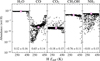 |
Fig. 1 Abundances of all samples at T=10 K, nH=105 cm−3, ζ= 1.3 × 10⁻¹⁷ s−1 and FUV=1 Habing at 104 years as function of the hydrogen diffusion barrier. Numbers at the bottom indicate rRIN and its 95% confidence intervals. Pink crosses indicate nominal abundances and hydrogen diffusion barrier. |
4 Results and discussion
4.1 Understanding the correlation coefficient
Figure 1 shows the abundances of a few major ice species at T= 10 K, nH=105 cm−3, ζ=1.3 × 10⁻¹⁷ s−1 and FUV=1 Habing at 104 years as a function of the sampled hydrogen diffusion barrier. Here, it can be seen that the H2O abundance as a function of the hydrogen diffusion barrier is a flat line, meaning that they are not correlated. On the other hand, there is a strong correlation between the CO abundance and H diffusion barrier, and this is indeed reflected in the value of rRIN.
Methanol, CH3OH, also shows a strong correlation, where the abundance at high H diffusion barriers (>425 K) decreases by nearly 10 orders of magnitude. This is an example of a non-linear correlation, also when using logarithmic abundances. As mentioned in Sect. 3.3, r without the RIN transformation underestimates the strength of this correlation, with r=−0.4 ± 0.11. This shows the need to use a rank-based correlation coefficient.
H2O, CH3OH and NH3 abundances all show a sharp decrease at H diffusion barriers above 425 K. At these high diffusion barriers, H becomes stationary, which leads to the unrealistic build-up of H ice up to an abundance of 10−4, which corresponds to about 102 monolayers. All carbon-, oxygen-, or nitrogen-bearing molecules are pushed to the bulk, where reactions are extremely slow due to the necessary diffusion of reagents through H2O. Thus, the abundance of larger species that rely on their formation on ices sharply decreases.
To illustrate the analysis workflow, we first show results for one set of physical conditions. The top panels in Fig. 2 present the abundances of five major ice species as function of time at T=10 K, nH=105 cm−3, ζ=1.3 × 10⁻¹⁷ s−1 and FUV= 1 Habing for all 1000 samples in black. The dashed pink lines indicate the abundance progression using the nominal network, whereas the light green lines show the log-average (or geometric mean) of all samples. All “strong” correlations, meaning |rRIN| ≥ 0.4, at any point in time are plotted in the bottom panels.
There is a considerable difference in the sensitivities before and after CO freeze-out, which occurs at around 104 years at this density. For example, the H2O abundance is first not sensitive to any parameter, however at 104 years becomes very sensitive to the N diffusion barrier.
It might not be immediately obvious why the H2O ice abundance is sensitive to the N diffusion barrier. Water and ammonia are mostly formed by multiple barrierless hydrogenations of O and N atoms, respectively. The nominal binding energies of atomic H and N are 650 and 720 K, respectively, meaning that the corresponding nominal diffusion barriers are 325 and 360 K. The main destruction pathways of atomic oxygen are through barrierless N+O → NO and O+H → OH. At later times, the gaseous O abundance is depleted because most of the oxygen is locked up in water already on the grain. Thus, the freeze-out rate of oxygen decreases and the abundance of surface abundance of O decreases from ∼ 10−6 to ∼ 6 × 10⁻⁹ with respect to hydrogen nuclei. This also happens because CO freeze-out pushes surface O to the bulk, where diffusion is much slower. Therefore, the very limited amount of surface O is used by the two reactions mentioned above, such that a more efficient N diffusion further depletes the amount of surface oxygen, and decreases the formation of OH and thus H2O. Additionally, with most of the CO frozen out, atomic H is consumed much faster by H+CO → HCO. This means that the two reactions mentioned above will swap in importance, that is to say, the ratio of the two reaction rates,  , goes up, and so the diffusion barrier of N becomes more important as well.
The opposite effect can be seen for the abundance of CO ice, where it is very sensitive to the hydrogen diffusion barrier at early times, and at later times that sensitivity is much weaker. CO on the grain is mainly formed and destroyed by HCO+H → CO+H2 and CO+H → HCO, respectively. A reaction between HCO and H can also form H2CO. At early times, when HCO forms and subsequently reacts with H, the abundance of CO will go down overall, because some will form H2CO. A higher diffusion barrier of atomic hydrogen will lead to a lower formation rate of HCO, and thus a higher abundance of CO (rRIN ≈ 0.9). At later times, however, the H abundance is so low that the correlation disappears. Methanol is still sensitive to the H diffusion barrier, because the abundance of methanol remains unchanged as all species are pushed to the bulk at 104 years and then reaches steady state due to the slow reactions in bulk ice.
NH3 is sensitive to the NH binding energy at early times. In the nominal network, the NH binding energy is 2600 K, which means that thermal desorption is negligible at 10 K. However, the barrierless reaction N+H → NH is quite exothermic (Δ Hreac= −88.43 kcal mol−1), and at these early times there is not yet a full monolayer of ice on the dust grains. Thus, ηCD, grainNH ≈ 0.56. Decreasing and increasing the binding energy of NH by 800 K changes the desorption probabilities to about 0.67 and 0.47, respectively, which will have a large effect on the NH abundance, and in turn on the abundance of NH3. At later times, this sensitivity disappears because the total ice abundance increases and the chemical desorption probability goes down. Then, NH3 is sensitive to the CH diffusion barrier at many physical conditions because of the barrierless reaction NH3+CH → CH2NH2, the main destruction pathway of NH3. The rate constant of this reaction, which is determined by the diffusion barrier of CH, imposes an upper limit on the NH3 abundance.
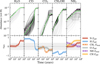 |
Fig. 2 Abundances (top) and correlation coefficients (bottom) of H2O, CO, CO2, CH3OH, and NH3 ices at T=10 K, nH=105 cm−3, ζ= 1.3 × 10⁻¹⁷ s−1 and FUV=1 Habing. In the top panels, the dashed pink line indicates the abundance using the nominal network, black lines indicate the individual samples, and light green is the log-average of all samples. In bottom subplots, the dashed gray line indicates perfectly uncorrelated parameters (rRIN=0), and the filled gray area indicates “weakly” correlated parameters (|rRIN|<0.4). The colored filled areas correspond to the 95% confidence intervals of the correlation coefficients. |
4.2 Across physical conditions
For the species of interest here, the correlations are relatively unaltered by changing the cosmic ray ionization rate (though this might not be the case at even higher rates, such as in the Central Molecular Zone; Le Petit et al. 2016). That is not to say that the abundances are unchanged by increasing the cosmic ray ionization rate, but the sensitivities are. Thus, for simplicity, we will continue discussing the abundance profiles and sensitivities using the standard rate of ζ=1.3 × 10⁻¹⁷ s−1. Similarly, the UV field strength has no effect on the ice abundances for densities above 104 cm−3 and no effect on the sensitivities at all physical conditions, so we will use 1 Habing for the rest of this work.
Figure 3 shows sensitivities for various physical conditions, as indicated above each set of panels. The temperature changes across the rows, whereas the density changes between the two columns. As expected, we observe that an increase in density mainly decreases the chemical timescale, and that the correlations are only affected to a limited extent. This can be seen by, for example, comparing Fig. 2 at nH=105 cm−3 and the top-right panel of Fig. 3 at nH=106 cm−3. On the other hand, changing the temperature allows other reactions to take over, such that each temperature has different sensitivities. For clarity, only 10, 30 and 50 K are shown in Fig. 3.
At 10 K and 103 cm−3 (top left in Fig. 3), many species are sensitive to the hydrogen diffusion barrier. There is no catastrophic CO freeze-out at this low density. This means that the H abundance on the surface is high, so species are still sensitive to its diffusion barrier. On the other hand, at higher densities, CO freeze-out depletes the H abundance, as mentioned in Sect. 4.1. The diffusion barriers of most species are too high for them to diffuse, so most species are stationary at this temperature. Small variations in the H diffusion barrier lead to large differences in the rate constants. For example, variation of the diffusion barrier between 350 and 450 K gives a difference in the rate constant of a factor ∼ 2 × 10⁴ (for the same prefactor) at 10 K. At 30 K, the same variation only results in a difference of a factor of 28. On the other hand, the variation of prefactors results in a factor of 104, which is why the abundances are more sensitive to the prefactors at 30 K.
The abundance of many species at 30 K and low density are correlated with the diffusion barrier of atomic oxygen. Since O is the more mobile reactant between C and O, some carbon- and oxygen-bearing species, such as CO2, rely on the diffusion of O to be formed on the ice. For example, the second most important formation reaction of CO2 at 30 K and nH=103 cm−3 is H2CO+ O → CO2+H2. Thus, a smaller diffusion barrier of O leads to a larger abundance of these species (rRIN<−0.4 at early times). On the other hand, the formation of water occurs mainly through diffusion of H, and lowering the diffusion of O atoms depletes the amount of oxygen (by formation of the species mentioned above) and thus lowers the H2O abundance (rRIN>0.4).
The CO abundance at 30 and 50 K and CO2 abundance at 50 K indicate the need for the use of accurate values for the desorption prefactor vdes. These are highly sensitive to the desorption prefactor, as indicated in the middle and bottom panels of Fig. 3, with a spread of about 4 orders of magnitude. This shows that the choice of prefactor is crucial, and astrochemical models need to use new chemical insight to calculate them (Minissale et al. 2022; Ligterink & Minissale 2023).
An interesting observation from Fig. 3 is that only one reaction energy barrier appears in these graphs, CO+OH → CO2+H(Ereac=1000 K). The maximum strength of correlation with this reaction is still quite weak, with rRIN ≈−0.45. This means that all other reaction barriers have correlations |rRIN|< 0.4 with all five species at all times and all of these six physical conditions. To confirm the insensitivity of abundances to reaction energy barriers, we repeated the calculations with only varying reaction energy barriers and keeping all other chemical parameters (binding energies, diffusion barriers, and prefactors) fixed. The results of these calculations are shown in Appendix D. The analysis here is limited to the total ice abundances, and the picture might be different if this is further differentiated to the surface and bulk abundances. The lack of correlations with reaction energy barriers is further discussed in Sect. 5.3.
4.3 Parameters showing strongest correlation
Many of the same parameters appear in Fig. 3. We have summarized these in Table 4. The references given in this table are by no means an exhaustive list (especially for H diffusion), but aim to give the reader an entry point into further reading.
We can compare our main correlations at 10 K with those of previous work. Comparing our results with those of Penteado et al. (2017), we find quite similar results. They find also the binding energy of C to be relevant, though they use a nominal binding energy of 715 K, and here a binding energy of 10 000 K corresponding to chemisorbed C−H2O is used. They find CH2 diffusion to be sensitive as well, but our results show CH is actually the more sensitive one due to the slightly higher values we use here for their binding energies. We did not have any correlation with the H2 binding energy, because we already included encounter desorption (Sect. 2.2). Iqbal et al. (2018) and Furuya et al. (2022a) also found the diffusion barriers of H, N, HCO, and O to constrain the predicted abundances. Instead of CH, they found the CH2 diffusion barrier, however that is also because the network they use makes CH2 more mobile than CH, whereas our network has the opposite behavior. Sil et al. (2024) calculated the binding energy of CH on H2O to be 2400 K, but Wakelam et al. (2017) found that CH barrierlessly reacts with H2O at a lower level of theory. Wakelam et al. (2017) also estimated the binding energy of CH2 to be 1400 K.
Of the parameters listed in Table 4, the H diffusion barrier has been investigated the most. Ásgeirsson et al. (2017) and Senevirathne et al. (2017) both investigated the diffusion of atomic hydrogen on crystalline and amorphous solid water using the same potential energy surface. They found diffusion to binding energy ratios of 0.64 and 0.37 respectively. This large difference is likely due to different surface structures. Al-Halabi & Van Dishoeck (2007) also investigated diffusion of H, and directly obtain the diffusion coefficient from molecular dynamics simulations.
The diffusion of atomic nitrogen on amorphous solid water was studied recently by Zaverkin et al. (2021), who found a ratio of 0.76. Pezzella et al. (2018) showed that the average diffusion barrier of atomic oxygen is 275 K, corresponding to a diffusion to binding energy ratio of around 0.3 using their binding energy. This confirms that there is no universal value for this ratio Furuya et al. (2022a), not even for atomic species, as used in most astrochemical models.
The diffusion barrier of HCO has not been studied explicitly. However, the binding energies of HCO reported in literature are larger than the ones used in this work. Thus, the diffusion of HCO is likely not as relevant as it appears from this study. We use a binding energy of 2400 K, as reported by Ferrero et al. (2020), whereas Bovolenta et al. (2022) reports a binding energy of around 1400 K. This large difference can likely be attributed to the different clusters, as the former uses a cluster with a cavity and the latter uses a spherical cluster of only 12−15 water molecules. Because HCO is formed from CO, it is most likely formed on a CO-rich surface. The strength of the interaction with a CO surface is lower than on H2O, meaning HCO diffuses more rapidly. To the best of our knowledge, the binding or diffusion of HCO on CO has not yet been studied.
The diffusion of CH3 was studied recently by Enrique-Romero & Lamberts (2025) on a small cluster of 14 H2O molecules. Due to the small cluster size, the binding energies and diffusion barriers can be best regarded as lower limits. Because they focused on the formation of CH3CN arising from short-range diffusion, the long-range diffusion of CH3 was not investigated.
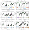 |
Fig. 3 Abundances (top) and correlation coefficients (bottom) of H2O, CO, CO2, CH3OH, and NH3 ices at various physical conditions indicated by the text above each subfigure. In the top panels, the dashed pink line indicates the abundance using the nominal network, black lines indicate the individual samples, and light green is the log-average of all samples. In bottom subplots, the dashed gray line indicates perfectly uncorrelated parameters (rRIN=0), and the filled gray area indicates “weakly” correlated parameters (|rRIN|<0.4). The color indicates which species or reaction the parameter belongs to, and the linestyle indicates its type. The colored filled areas correspond to the 95% confidence intervals of the correlation coefficients. Legends are the same for all panels. |
Selection of chemical parameters that many species are correlated with, and the temperature(s) at which they were found to be have strong correlations with ice abundances.
4.4 Limitations
Nondiffusive chemistry means that reactions can take place between any two reactants in proximity. For example, after a reaction has taken place, the product(s) of that reaction can again react with other close-by species. This means that diffusion of heavy radicals is not necessary to produce larger molecules, such as complex organic molecules; thus, it allows for their formation at lower temperatures. Diffusion is still necessary for the formation of the radicals. This is inherently present in kinetic Monte Carlo simulations, which can reproduce laboratory experiments at low temperatures where diffusion of larger radicals is slow (Fedoseev et al. 2015, 2017; Simons et al. 2020; Ioppolo et al. 2020). It has recently been implemented into rate equation models (Jin & Garrod 2020), but was not considered in this work. We expect that if it were, the correlations of abundances with binding energies of weakly bound species would increase because the nondiffusive chemistry would lead to cyclic H abstraction and addition, making chemical desorption more efficient (see Sect 4.1 of Jin & Garrod 2020). This also means that the abundances would become more sensitive to how chemical desorption is treated. On the other hand, we expect that correlations with diffusion barriers of larger radicals (e.g., HCO and CH3) to become less important because as a radical is formed, it can react with other radicals without needing to overcome diffusion barriers. As shown in Fig. 9 of Borshcheva et al. (2025), molecular diffusion barriers indeed matter less in the nondiffusive framework. However, larger molecules such as complex organic molecules are likely most affected by this. Occupation of deeper binding sites by other species can also greatly speed up diffusion (see for example Karssemeijer et al. 2013; Zaverkin et al. 2021) and is not taken into account in current astrochemical models.
Besides Langmuir–Hinshelwood reactions, chemistry on ices can also occur through Eley–Rideal reactions. Eley–Rideal reactions can occur when a species from the gas-phase adsorbs on the surface of the ice next to or on top of an already adsorbed species. In the network used here, there is a very limited number of Eley–Rideal reactions, meaning that chemistry must be driven by Langmuir–Hinshelwood (diffusive) reactions. Including more Eley–Rideal reactions might increase the importance of energy barriers. However, because Eley–Rideal reactions rely on collisions with the adsorbates, this is likely to be most important for major ice species such as CO.
Varying the reaction energy barrier affects the tunneling probability, and thus the reaction rate. However, we note that the tunneling probability estimated with the rectangular barrier approximation can be off by orders of magnitude compared to quantum chemical instanton calculations. For example, using Eq. (1) from Lamberts et al. (2017) and data there-in, we find an instanton tunneling probability of ∼ 4 × 10⁻⁹ at 10 K for CH4+ OH → CH3+H2O. Using the energy barrier they calculated using density functional theory (2575 K) and the rectangular barrier approximation, we find Preac ≈ 3 × 10⁻¹³. Decreasing this barrier by 800 K increases the probability to ∼ 4 × 10⁻¹¹, still two orders of magnitude off from the instanton probability. An “effective” energy barrier, the energy barrier that results in a correct tunneling probability from Eq. (5), or Model 3 suggested in Zheng & Truhlar (2010) for correct temperature dependence could be used, but for many reactions no tunneling probabilities are available.
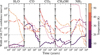 |
Fig. 4 Width of the 68.27% confidence intervals of abundances of selected ice species at various temperatures (averaged over all densities) over time at ζ=1.3 × 10⁻¹⁷ s−1 and FUV=1 Habing. The solid, dashed, dotted, dashed-dotted, and densely dotted lines correspond to 10, 20, 30, 40 and 50 K, respectively. The dashed gray line indicates a width of two orders of magnitude. |
5 Implications
5.1 Poorly constrained species
As mentioned in Sect. 3.2, we are not able to give quantitative uncertainties of the abundances. Nevertheless, qualitative uncertainties are still very beneficial to properly constrain physical parameters of observed clouds. At 10 K, the abundance of H2O is quite insensitive to changes in the ice chemistry, such that observations of H2O ice can be accurately fitted. On the other hand, the abundances of CO and CH3OH are very sensitive to changes in the network (see for example the top row of Fig. 3), such that fits of observations are also sensitive to changes in the network. We note again that the hydrogen diffusion barrier is varied with 162.5 K in either direction, and this is a similar change as going from  to
to  . This small (in terms of energy) change in hydrogen diffusion barrier has an extremely large effect on many species at 10 K. At 20 K and above, variations of diffusion barriers of larger species start to strongly affect the predicted abundances. Figure 4 shows the width, meaning the ratio of the upper limit to the lower limit, of the 68.27% confidence interval of abundances at various temperatures, averaged over all densities. In general, the width goes down at later times, because these species are mostly consumed by reactions. It is clear that the abundances are often uncertain to within two to four orders of magnitude.
This shows the risk of extracting chemical parameters from comparisons between models and observations, such as a diffusion barrier to binding energy ratio (Garrod & Pauly 2011; Borshcheva et al. 2025). From our sensitivity analysis, we conclude that observations of specific species cannot determine a ratio χ that is universal for all atoms and molecules.
5.2 Assumptions in models
Astrochemically relevant ices (e.g., amorphous solid water) do not have unique binding sites, but have a distribution of binding sites with various depths and probabilities (Amiaud et al. 2006; He et al. 2016; Minissale et al. 2022). Early attempts to include this in astrochemical models relied on treating the species in different binding sites as entirely different species in the network (i.e., with separate abundances and reactions), with rates connecting them (Cuppen & Garrod 2011; Grassi et al. 2020). This made it too computationally expensive to do so for every species. Furuya (2024) developed an efficient method to include binding energy distributions. While we did not take binding energy distributions into account, we still probe whether a species will be strongly affected by including distributions. It is important for the binding energy distributions to be well-studied and implemented, as simply assuming a normal distribution is not valid for many species (see e.g., Bovolenta et al. 2022; Enrique-Romero & Lamberts 2024) and even the assumed width of the distribution has an effect on the abundances (see Figs. 6 and 7 of Furuya 2024). Species that are strongly correlated with binding energies or diffusion barriers will be affected by the assumed distributions.
Recently, there have been multiple works that vary the binding energy and, as a result, the diffusion barrier of species by the amount of CO in the ice (see e.g., Molpeceres et al. 2024). This becomes especially important after the catastrophic CO freeze-out has occurred, which greatly increases the abundance of CO on the surface, thus decreasing the interaction strength of adsorbates with the ice surface. Some works simply assume ratios of the interaction strengths  for all species (see, e.g., Kalvāns et al. 2024), although this should be done with care because, as shown above, assumptions about diffusion barriers greatly influence the calculated abundances. Thus, for scaling the binding energy by the amount of CO, we recommend using the method by Molpeceres et al. (2024), where the binding energies of species of interest on CO are calculated using density functional theory, and verifying that varying the binding energy on CO in the model of other species does not affect abundances.
5.3 Recommendations for experiments and calculations
One of the main findings is that the calculated ice abundances of many species are not sensitive to reaction energy barriers. That means that getting accurate reaction energy barriers (using e.g., high-level density functional theory) is often not necessary. This also applies to complex organic molecules, as discussed in Appendix C.
This is because of the treatment of competition. Consider a Langmuir–Hinshelwood reaction between i and j, where i has a lower diffusion barrier. At low diffusion barriers, the diffusion rate ( , Eq. (3)) becomes much larger than the reaction rate κi+j if the reaction has a barrier. Thus, the fraction describing competition (Eq. (6)) can be approximated as
  , and the resulting reaction rate constant (Eq. (7)) becomes approximately
 (23)
independent of the diffusion rate. On the other hand, reactions with a low energy barrier or for which the diffusion barriers of the reagents are high have
(23)
independent of the diffusion rate. On the other hand, reactions with a low energy barrier or for which the diffusion barriers of the reagents are high have  , such that
 (24)
independent of κi+j and thus the reaction barrier height. In other words, the reaction rate constant
(24)
independent of κi+j and thus the reaction barrier height. In other words, the reaction rate constant  is proportional to the rate of the slowest process.
Figure 5 shows the ratio between the reaction probability (Eq. (5)) and the Boltzmann factor for diffusion at 10 K. Low ratios, indicated by green, correspond to the fast diffusion limit (Eq. (23)) and high ratios, indicated by purple, correspond to the slow diffusion limit (Eq. (24)). We neglect the influence of the prefactors in this figure, meaning that we show the ratio of the reaction probability to the diffusion probability, and not their respective rate constants. The exact values of the tunneling mass μ in Fig. 5 are not important, but two examples are shown to indicate how the tunneling efficiency affects the trend. For reactions where tunneling through the reaction energy barrier is inefficient; for instance, if a carbon atom is being exchanged (μ=12 amu, shown in Fig. 5), the height of the reaction energy barrier has more of an effect on the ratio. Many relevant reactions on ices, especially at this low temperature, have a reaction barrier below 1000 K to 2000 K, tunneling mass of μ=1 amu and reagents with diffusion barriers above 300 K. Thus, they fall in the slow-diffusion limit, where Preac ≫ exp (−Ediff/T), and their reaction rates are dictated mainly by the rate of diffusion of the most mobile species according to Eq. (24). This means that an accurate reaction probability, calculated with for example instanton theory (e.g., in Lamberts et al. 2017), or an exact energy barrier for the reaction is not necessary. On the other hand, if there is reason to suspect that the reaction might occur in the fast-diffusion limit (green in Fig. 5), for example because it has a very high barrier or involves movement of relatively heavy atoms making tunneling inefficient, then the actual reaction probability becomes more important. However, these reactions are generally less important for the ice chemistry. At higher temperatures these regimes shift further down and right, because diffusion is a temperature-dependent process whereas the reactions are often tunneling-dominated and so temperature-independent.
To give an example, the CO2 abundance at 50 K correlates with the reaction barrier of CO+OH → CO2+H, as can be seen in the bottom-left panel of Fig. 3. At the nominal CO and OH diffusion barriers and energy barrier (1000 K), the ratio between the sum of the diffusion rate constants and the reaction rate constant is around 2 × 10⁻³, in the fast diffusion regime. On the other hand, at the minimum of the range of its energy barrier, the ratio becomes around 50, in the slow diffusion regime. Thus, the height of the reaction barrier is important for the abundance of CO2.
This means that once the diffusion barriers are properly constrained, accurate reaction energy barriers are often not required to have robust chemical models. After an approximate calculation (using, e.g., a lower accuracy density functional or machine-learned interatomic potential) or measurement has been done, it can be decided if it needs closer investigation. If the reaction falls in the slow diffusion regime at the physical conditions the reactants are expected to be available, it is probably not needed to obtain a more accurate energy barrier. On the other hand, if the reaction falls close to the switch or in the fast diffusion regime, a more accurate energy barrier might be necessary. We note again that this is a diffusive rate equation model that has no microscopic detail. In a model with more microscopic detail, for example kinetic Monte Carlo, where explicit competition between different reactions is taken into account, the situation might be different.
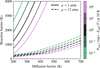 |
Fig. 5 Ratio between the reaction probability (Eq. (5)) and the Boltzmann factor for diffusion at 10 K, for reactions with different energy barriers and diffusion barrier of the most mobile reagent. Solid lines indicate a reaction where tunneling is efficient (μ=1 amu), and dashed lines indicate a reaction where tunneling is inefficient (μ=12 amu). |
6 Summary and conclusions
We investigated the correlation of abundances of ice species with binding energies, diffusion barriers, and reaction energy barriers, as well as the desorption and diffusion prefactors. We also improved the treatment of interstellar ice chemistry in UCLCHEM by updating the chemical desorption formalism, limiting the amount of H2 on the surface, including an improved calculation of the tunneling probability, and correctly calculating the desorption prefactors. We summarize the main findings of this work below.
Ice chemistry in rate equation based astrochemical models for prestellar objects is mainly sensitive to diffusion of small radicals such as H, N, O, CH3, and HCO. More attention needs to be given to accurate calculation or measurement of the diffusion barrier of these larger radicals.
In many cases, accurate energy barriers for reactions are not essential because diffusion is actually the rate-limiting step. This means that reaction energy barriers can be determined using more approximate methods. Depending on whether it is faster or not than the hopping rate, a more accurate barrier needs to be determined.
Fitting binding energies, diffusion barriers or reaction energy barriers from observations is extremely risky because of the complex interplay of many parameters. When trying to constrain parameters, the observed species need to be sensitive to the parameters.
Care needs to be taken when fitting observed abundances to obtain physical conditions because the modeled abundances of some species are highly sensitive to the chemical parameters in the network. This could lead to differences in determined physical conditions when using different astrochemical codes or networks.
Overall, we have done an extensive sensitivity analysis of ice chemistry in rate-equation based astrochemical models. To get more accurate astrochemical models, more accurate diffusion barriers need to be determined.
Acknowledgements
T.M.D. is financially supported by the Dutch Astrochemistry Network of the Dutch Research Council (NWO) under grant no. ASTRO.JWST.001. S.V. acknowledges funding from the European Research Council (ERC) under the European Union’s Horizon 2020 research and innovation programme MOPPEX 833460. The authors thank Kenji Furuya and Germán Molpeceres for fruitful discussions. Software. UCLCHEM (Holdship et al. 2017), NumPy (Harris et al. 2020), Matplotlib (Hunter 2007), SciPy (Virtanen et al. 2020), pandas (The pandas development team 2020).
References
- Al-Halabi, A., & Van Dishoeck, E. F., 2007, MNRAS, 382, 1648 [NASA ADS] [CrossRef] [Google Scholar]
- Amiaud, L., Fillion, J. H., Baouche, S., et al. 2006, JChPh, 124 [Google Scholar]
- Angeli, D., 2009, Eur. J. Control, 15, 398 [Google Scholar]
- Ásgeirsson, V., Jónsson, H., & Wikfeldt, K. T., 2017, JPCC, 121, 1648 [Google Scholar]
- Asplund, M., Grevesse, N., Sauval, A. J., & Scott, P., 2009, ARA&A, 47, 481 [CrossRef] [Google Scholar]
- Bishara, A. J., & Hittner, J. B., 2012, Psychol. Methods, 17, 399 [CrossRef] [Google Scholar]
- Bliss, C. I., 1967, Statistics in Biology. Statistical Methods for Research in the Natural Sciences (McGraw-Hill Book Company), xiv+558 [Google Scholar]
- Borshcheva, K., Fedoseev, G., Punanova, A. F., et al. 2025, ApJ, 990, 163 [Google Scholar]
- Bovolenta, G. M., Vogt-Geisse, S., Bovino, S., & Grassi, T., 2022, ApJS, 262, 17 [NASA ADS] [CrossRef] [Google Scholar]
- Brown, P. N., Byrne, G. D., & Hindmarsh, A. C., 1989, SIAM J. Sci. Statist. Comput., 10, 1038 [Google Scholar]
- Byrne, A. N., Xue, C., Van Voorhis, T., & McGuire, B. A., 2024, PCCP, 26, 26734 [Google Scholar]
- Chang, Q., Cuppen, H. M., & Herbst, E., 2007, A&A, 469, 973 [NASA ADS] [CrossRef] [EDP Sciences] [Google Scholar]
- Cuppen, H. M., & Garrod, R. T., 2011, A&A, 529, A151 [NASA ADS] [CrossRef] [EDP Sciences] [Google Scholar]
- Cuppen, H. M., & Herbst, E., 2007, ApJ, 668, 294–309 [NASA ADS] [Google Scholar]
- Cuppen, H. M., Walsh, C., Lamberts, T., et al. 2017, Space Sci. Rev., 212, 1 [Google Scholar]
- Curtiss, L. A., Redfern, P. C., Smith, B. J., & Radom, L., 1996, JChPh, 104, 5148 [Google Scholar]
- Dobrijevic, M., Hébrard, E., Plessis, S., et al. 2010, Adv. Space Res., 45, 77 [NASA ADS] [CrossRef] [Google Scholar]
- Efron, B., & Tibshirani, R., 1994, An Introduction to the Bootstrap (Chapman and Hall/CRC) [Google Scholar]
- Enrique-Romero, J., & Lamberts, T., 2024, JPCL, 15, 7799 [Google Scholar]
- Enrique-Romero, J., & Lamberts, T., 2025, A&A, 699, A235 [NASA ADS] [CrossRef] [EDP Sciences] [Google Scholar]
- Enrique-Romero, J., Rimola, A., Ceccarelli, C., et al. 2022, ApJS, 259, 39 [NASA ADS] [CrossRef] [Google Scholar]
- Fedoseev, G., Cuppen, H. M., Ioppolo, S., Lamberts, T., & Linnartz, H., 2015, MNRAS, 448, 1288 [NASA ADS] [CrossRef] [Google Scholar]
- Fedoseev, G., Chuang, K.-J., Ioppolo, S., et al. 2017, ApJ, 842, 52 [NASA ADS] [CrossRef] [Google Scholar]
- Ferrero, S., Zamirri, L., Ceccarelli, C., et al. 2020, ApJ, 904, 11 [NASA ADS] [CrossRef] [Google Scholar]
- Ferrero, S., Pantaleone, S., Ceccarelli, C., et al. 2023, ApJ, 944, 142 [NASA ADS] [CrossRef] [Google Scholar]
- Fredon, A., Lamberts, T., & Cuppen, H. M., 2017, ApJ, 849, 125 [NASA ADS] [CrossRef] [Google Scholar]
- Fredon, A., Radchenko, A. K., & Cuppen, H. M., 2021, AcChR, 54, 745 [Google Scholar]
- Furuya, K., 2024, ApJ, 974, 115 [NASA ADS] [CrossRef] [Google Scholar]
- Furuya, K., Hama, T., Oba, Y., et al. 2022a, ApJ, 933, L16 [CrossRef] [Google Scholar]
- Furuya, K., Oba, Y., & Shimonishi, T. 2022b, ApJ, 926, 171 [NASA ADS] [CrossRef] [Google Scholar]
- Garrod, R. T., 2013, ApJ, 765, 60 [Google Scholar]
- Garrod, R. T., & Pauly, T., 2011, ApJ, 735, 15 [Google Scholar]
- Garrod, R. T., Belloche, A., Müller, H. S. P., & Menten, K. M., 2017, A&A, 601, A48 [NASA ADS] [CrossRef] [EDP Sciences] [Google Scholar]
- Ghesquière, P., Mineva, T., Talbi, D., et al. 2015, PCCP, 17, 11455 [Google Scholar]
- Gould, R. J., 1963, PhD thesis, Cornell University [Google Scholar]
- Grassi, T., Bovino, S., Caselli, P., et al. 2020, A&A, 643, A155 [EDP Sciences] [Google Scholar]
- Hama, T., Kuwahata, K., Watanabe, N., et al. 2012, ApJ, 757, 185 [NASA ADS] [CrossRef] [Google Scholar]
- Harris, C. R., Millman, K. J., van der Walt, S. J., et al. 2020, Nature, 585, 357 [NASA ADS] [CrossRef] [Google Scholar]
- Hasegawa, T. I., Herbst, E., & Leukng, C. M., 1992, ApJS, 82, 167 [NASA ADS] [CrossRef] [Google Scholar]
- He, J., Acharyya, K., & Vidali, G., 2016, ApJ, 825, 89 [Google Scholar]
- Heyl, J., Holdship, J., & Viti, S., 2022, ApJ, 931, 26 [NASA ADS] [CrossRef] [Google Scholar]
- Hincelin, U., Chang, Q., & Herbst, E., 2015, A&A, 574, A24 [NASA ADS] [CrossRef] [EDP Sciences] [Google Scholar]
- Holdship, J., Viti, S., Jiménez-Serra, I., Makrymallis, A., & Priestley, F., 2017, ApJ, 154, 38 [CrossRef] [Google Scholar]
- Holdship, J., Jeffrey, N., Makrymallis, A., Viti, S., & Yates, J., 2018, ApJ, 866, 116 [NASA ADS] [CrossRef] [Google Scholar]
- Hunter, J. D., 2007, Comput. Sci. Eng., 9, 90 [NASA ADS] [CrossRef] [Google Scholar]
- Ioppolo, S., Fedoseev, G., Chuang, K.-J., et al. 2020, Nat. Astron., 5, 197 [NASA ADS] [CrossRef] [Google Scholar]
- Iqbal, W., Wakelam, V., & Gratier, P., 2018, A&A, 620, A109 [NASA ADS] [CrossRef] [EDP Sciences] [Google Scholar]
- Jenkins, E. B., 2009, ApJ, 700, 1299 [Google Scholar]
- Jin, M., & Garrod, R. T., 2020, ApJS, 249, 26 [Google Scholar]
- Johnson III, R. D., 2022, NIST Computational Chemistry Comparison and Benchmark Database [Google Scholar]
- Kalvāns, J., Kalniņa, A., & Veitners, K., 2024, A&A, 687, A296 [NASA ADS] [CrossRef] [EDP Sciences] [Google Scholar]
- Karssemeijer, L. J., Ioppolo, S., van Hemert, M. C., et al. 2013, ApJ, 781, 16 [Google Scholar]
- Kimura, H., Mann, I., & Jessberger, E. K., 2003, ApJ, 582, 846 [CrossRef] [Google Scholar]
- Kouchi, A., Furuya, K., Hama, T., et al. 2020, ApJ, 891, L22 [NASA ADS] [CrossRef] [Google Scholar]
- Kuntz, P. J., Mitchell, G. F., & Ginsburg, J., 1976, ApJ, 209, 116 [Google Scholar]
- Lamberts, T., Fedoseev, G., Kästner, J., Ioppolo, S., & Linnartz, H., 2017, A&A, 599, A132 [NASA ADS] [CrossRef] [EDP Sciences] [Google Scholar]
- Lamberts, T., Markmeyer, M. N., Kolb, F. J., & Kästner, J., 2019, ACS Earth Space Chem., 3, 958 [Google Scholar]
- Le Petit, F., Ruaud, M., Bron, E., et al. 2016, A&A, 585, A105 [NASA ADS] [CrossRef] [EDP Sciences] [Google Scholar]
- Ligterink, N. F. W., & Minissale, M., 2023, A&A, 676, A80 [NASA ADS] [CrossRef] [EDP Sciences] [Google Scholar]
- Ligterink, N. F. W., Walsh, C., Cuppen, H. M., et al. 2025, PCCP, 27, 19630 [Google Scholar]
- Löfgren, P., Ahlström, P., Lausma, J., Kasemo, B., & Chakarov, D., 2002, Langmuir, 19, 265 [Google Scholar]
- May, R. A., Smith, R. S., & Kay, B. D., 2012, J. Phys. Chem. Lett., 3, 327 [Google Scholar]
- Millar, T. J., Walsh, C., Van de Sande, M., & Markwick, A. J., 2024, A&A, 682, A109 [NASA ADS] [CrossRef] [EDP Sciences] [Google Scholar]
- Minissale, M., Dulieu, F., Cazaux, S., & Hocuk, S., 2015, A&A, 585, A24 [Google Scholar]
- Minissale, M., Aikawa, Y., Bergin, E., et al. 2022, ACS ESC, 6, 597 [Google Scholar]
- Molpeceres, G., Zaverkin, V., Furuya, K., Aikawa, Y., & Kästner, J., 2023, A&A, 673, A51 [NASA ADS] [CrossRef] [EDP Sciences] [Google Scholar]
- Molpeceres, G., Furuya, K., & Aikawa, Y., 2024, A&A, 688, A150 [NASA ADS] [CrossRef] [EDP Sciences] [Google Scholar]
- Morata, O., & Hasegawa, T. I., 2013, MNRAS, 429, 3578 [Google Scholar]
- Müller, H. S., Schlöder, F., Stutzki, J., & Winnewisser, G., 2005, JMoSt, 742, 215 [Google Scholar]
- Neese, F., 2025, WIREs Computat. Mol. Sci., 15, e70019 [Google Scholar]
- O’Boyle, N. M., Banck, M., James, C. A., et al. 2011, J. Cheminformatics, 3, 33 [CrossRef] [Google Scholar]
- Padovani, M., Ivlev, A. V., Galli, D., & Caselli, P., 2018, A&A, 614, A111 [NASA ADS] [CrossRef] [EDP Sciences] [Google Scholar]
- Pantaleone, S., Enrique-Romero, J., Ceccarelli, C., et al. 2020, ApJ, 897, 56 [NASA ADS] [CrossRef] [Google Scholar]
- Penteado, E. M., Walsh, C., & Cuppen, H. M., 2017, ApJ, 844, 71 [Google Scholar]
- Pezzella, M., Unke, O. T., & Meuwly, M., 2018, J. Phys. Chem. L., 9, 1822 [Google Scholar]
- Quénard, D., Jiménez-Serra, I., Viti, S., Holdship, J., & Coutens, A., 2018, MNRAS, 474, 2796 [Google Scholar]
- Riedel, W., Sipilä, O., Redaelli, E., et al. 2023, A&A, 680, A87 [NASA ADS] [CrossRef] [EDP Sciences] [Google Scholar]
- Ruaud, M., Wakelam, V., & Hersant, F., 2016, MNRAS, 459, 3756 [Google Scholar]
- Ruscic, B., & Bross, D., 2025, Active Thermochemical Tables (ATcT) values based on ver. 1.220 of the Thermochemical Network [Google Scholar]
- Saltelli, A., Aleksankina, K., Becker, W., et al. 2019, EnvMS, 114, 29 [Google Scholar]
- Senevirathne, B., Andersson, S., Dulieu, F., & Nyman, G., 2017, MolAs, 6, 59 [Google Scholar]
- Sil, M., Roy, A., Gorai, P., et al. 2024, A&A, 690, A252 [NASA ADS] [CrossRef] [EDP Sciences] [Google Scholar]
- Simons, M. A. J., Lamberts, T., & Cuppen, H. M., 2020, A&A, 634, A52 [NASA ADS] [CrossRef] [EDP Sciences] [Google Scholar]
- Sobol’, I., 1967, USSR Computat. Math. Math. Phys., 7, 86 [CrossRef] [Google Scholar]
- Spearman, C., 1904, AmJPsy, 15, 72 [Google Scholar]
- The pandas development team 2020, pandas-dev/pandas: Pandas [Google Scholar]
- Tielens, A. G. G. M., & Allamandola, L. J., 1987, Composition, Structure, and Chemistry of Interstellar Dust (Springer Netherlands), 397 [Google Scholar]
- Vasyunin, A. I., Semenov, D., Henning, T., et al. 2008, ApJ, 672, 629 [Google Scholar]
- Vermariën, G., Viti, S., Heyl, J., & Fontani, F., 2025, A&A, 699, A18 [NASA ADS] [CrossRef] [EDP Sciences] [Google Scholar]
- Virtanen, P., Gommers, R., Oliphant, T. E., et al. 2020, NatMe, 17, 261 [NASA ADS] [Google Scholar]
- Wakelam, V., Herbst, E., & Selsis, F., 2006, A&A, 451, 551 [NASA ADS] [CrossRef] [EDP Sciences] [Google Scholar]
- Wakelam, V., Herbst, E., Le Bourlot, J., et al. 2010, A&A, 517, A21 [NASA ADS] [CrossRef] [EDP Sciences] [Google Scholar]
- Wakelam, V., Loison, J.-C., Mereau, R., & Ruaud, M., 2017, MolAs, 6, 22 [NASA ADS] [Google Scholar]
- Wakelam, V., Gratier, P., Loison, J.-C., et al. 2024, A&A, 689, A63 [NASA ADS] [CrossRef] [EDP Sciences] [Google Scholar]
- Yoshikawa, N., & Hutchison, G. R., 2019, J. Cheminformatics, 11, 49 [Google Scholar]
- Zaverkin, V., Molpeceres, G., & Kästner, J., 2021, MNRAS, 510, 3063 [Google Scholar]
- Zheng, J., & Truhlar, D. G., 2010, PCCP, 12, 7782 [Google Scholar]
Chemical accuracy is the accuracy required to match or exceed experimental accuracy and to make realistic chemical predictions. It is often taken to be 1 kcal mol−1 ≈ 500 K.
Appendix A Estimation of tunneling mass
For a Langmuir–Hinshelwood reaction, the mass of the tunneling “particle” is essential in correctly calculating the rate constant. In most astrochemical models, the mass of the tunneling particle is taken as the reduced mass of the two reagents (Hasegawa et al. 1992; Ruaud et al. 2016),
 (A.1)
However, this strongly overestimates the mass of the tunneling particle (and so underestimates the rate constant) for some reactions. For example, the reagents of reaction CH4+OH → CH3+H2O have a reduced mass of ∼ 8 amu, while the tunneling particle is a hydrogen atom (moving from CH4 to the OH radical) and so to get an accurate tunneling probability a tunneling particle mass of 1 amu should be used instead. With a barrier of 2575 K (Lamberts et al. 2017), using the reduced mass results in a tunneling probability underestimated by ∼ 23 orders of magnitude, whereas using μ=1 amu underestimates the reaction rate constant by about 4 orders of magnitude. To remedy this, we estimate the tunneling mass of a Langmuir–Hinshelwood reaction using the following method, similar to Garrod et al. (2017). For a one-product reaction, we simply use Eq. (A.1). For a two-product reaction, find which reagent is most similar to which product. If the difference between a reagent and the corresponding product is one atom, that atom has been exchanged between the two reagents, and so the tunneling mass is set to the mass of that atom. If not, Eq. (A.1) is used. This method does not always decrease the tunneling mass. For example, for H + O2H → 2 OH, the predicted tunneling mass is mO = 16 amu, whereas the reduced mass of the reagents is ∼ 1 amu. Barrierless reactions are unaffected because their tunneling probability is unity, regardless of the tunneling mass.
(A.1)
However, this strongly overestimates the mass of the tunneling particle (and so underestimates the rate constant) for some reactions. For example, the reagents of reaction CH4+OH → CH3+H2O have a reduced mass of ∼ 8 amu, while the tunneling particle is a hydrogen atom (moving from CH4 to the OH radical) and so to get an accurate tunneling probability a tunneling particle mass of 1 amu should be used instead. With a barrier of 2575 K (Lamberts et al. 2017), using the reduced mass results in a tunneling probability underestimated by ∼ 23 orders of magnitude, whereas using μ=1 amu underestimates the reaction rate constant by about 4 orders of magnitude. To remedy this, we estimate the tunneling mass of a Langmuir–Hinshelwood reaction using the following method, similar to Garrod et al. (2017). For a one-product reaction, we simply use Eq. (A.1). For a two-product reaction, find which reagent is most similar to which product. If the difference between a reagent and the corresponding product is one atom, that atom has been exchanged between the two reagents, and so the tunneling mass is set to the mass of that atom. If not, Eq. (A.1) is used. This method does not always decrease the tunneling mass. For example, for H + O2H → 2 OH, the predicted tunneling mass is mO = 16 amu, whereas the reduced mass of the reagents is ∼ 1 amu. Barrierless reactions are unaffected because their tunneling probability is unity, regardless of the tunneling mass.
Appendix B Entalpies of formation
If the enthalpy of formation of a species was unavailable in databases, it was instead calculated using quantum chemical methods. First, the (approximately) optimal geometry was generated from the SMILES code using OpenBabel’s 3D conformer generation (O’Boyle et al. 2011; Yoshikawa & Hutchison 2019). The precision of the generated atomic coordinates was then reduced to 3 decimal places to prevent ORCA from placing incorrect symmetry constraints during further geometry optimizations. High accuracy energies were then calculated for the molecules and the atoms they are composed of using the G2(MP2,SVP) method, as described by Curtiss et al. (1996). This method consists of geometry optimizations, a zero-point vibrational energy calculation, and high-accuracy single-point calculations, resulting in E0. The calculations were carried out in ORCA version 6.1.0 (Neese 2025), with the compound[G2-MP2-SVP] keyword. This is done for the two lowest multiplicities (i.e., multiplicities of 1 and 3 for a species with an even number of electrons, and multiplicities of 2 and 4 for species with an odd number of electrons) to find the true electronic ground state. The enthalpy of formation of a molecule, AxByCz, is then
 (B.1)
where the enthalpies of formation of atoms A, B and C are experimental values taken from the Active Thermochemical Tables (ATcT, Ruscic & Bross 2025). The effect of a non-zero temperature is neglected. Figure B.1 compares literature values for the enthalpies of formation from ATcT with values calculated with G2(MP2,SVP). This method is clearly accurate enough, even for open-shell molecules, with a mean absolute deviation of only 1.31 kcal mol−1, which is just above “chemical accuracy.” The enthalpies of formation are only used here for determining the chemical desorption probability, and are therefore less critical. The newly calculated enthalpies of formation are shown in Table B.1. The code to calculate enthalpies of formation of new species is available on GitHub6.
(B.1)
where the enthalpies of formation of atoms A, B and C are experimental values taken from the Active Thermochemical Tables (ATcT, Ruscic & Bross 2025). The effect of a non-zero temperature is neglected. Figure B.1 compares literature values for the enthalpies of formation from ATcT with values calculated with G2(MP2,SVP). This method is clearly accurate enough, even for open-shell molecules, with a mean absolute deviation of only 1.31 kcal mol−1, which is just above “chemical accuracy.” The enthalpies of formation are only used here for determining the chemical desorption probability, and are therefore less critical. The newly calculated enthalpies of formation are shown in Table B.1. The code to calculate enthalpies of formation of new species is available on GitHub6.
Newly calculated enthalpies of formation using the method described in Appendix B.
 |
Fig. B.1 Comparison of enthalpies of formation from ATcT and calculated using the method described in Appendix B. Blue circles indicate molecules with an even number of electrons, whereas red crosses indicate molecules with an odd number of electrons. The dashed gray line indicates a perfect agreement. |
Appendix C Complex organic molecules
Complex organic molecules (COMs) are organic molecules consisting of six or more atoms. They are believed to be important precursors for the formation of biologically relevant molecules that might lead to the emergence of life.
Figure C.1 shows sensitivities at different physical conditions for various COMs. At low temperature (10 K), many COMs are sensitive to the diffusion barrier of atomic H. If the H diffusion barrier is higher, their abundance is too. These COMs are mostly formed by barrierless recombination of smaller radicals, such as CH3+CHO → CH3CHO. The abundance of these radicals is governed by the rate of their hydrogenation, for example CH3+H → CH4 or CHO+H → H2CO/CO+H2. Because these larger radicals are more strongly bound to the surface than atomic hydrogen, the reaction rate is mainly determined by the H diffusion rate. If the hydrogen diffusion barrier is higher, these hydrogenation reactions will occur slower and as a result the abundance of these radicals are larger, such that the abundance of the resulting COMs is also larger. This was also found by Furuya (2024) and Jin & Garrod (2020).
At 30 K, the abundance of H on the ice is low and its diffusion occurs rapidly, and the limiting step becomes the diffusion of the larger radicals. This means that many COMs are sensitive to the diffusion barriers of the reagent radicals. For example, CH3CHO is very sensitive to the CH3 diffusion barrier, because it is the more mobile one of the two reagents that react to form it. On the other hand, HCOOCH3 is more sensitive to the diffusion barrier of HCO than the one of CH3O because CH3O is more strongly bound to the surface.
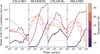 |
Fig. C.2 Width of the 68.27% confidence intervals of abundances of some complex organic molecules at various temperatures (averaged over all densities) over time at ζ=1.3 × 10⁻¹⁷ s−1 and FUV=1 Habing. The solid, dashed, dotted, dashed-dotted, and densely dotted lines correspond to 10, 20, 30, 40 and 50 K, respectively. The dashed gray line indicates a width of 2 orders of magnitude. |
At 50 K, the situation is similar, but now also the desorption of atomic hydrogen is important. Higher desorption prefactors lead to a lower abundance of atomic hydrogen on the ice, which leads to a lower rate of radical destruction. This in turn, as was the case at 10 K, leads to a higher abundance of COMs.
Figure C.2 shows the widths of the 68.27% confidence intervals of abundances. This shows that these complex organic molecules are extremely sensitive to the network being used. Especially at 20 K, where diffusion of HCO is either possible or not possible depending on its diffusion barrier, the uncertainties of HCOOCH3 and NH2CHO are extremely large.
Appendix D Variation of reaction energy barriers
To confirm that the abundances are not sensitive to the reaction energy barriers, we repeated the same calculations, but only varying the reaction energy barriers and keeping the binding energies, diffusion barriers and the prefactors fixed to their nominal values. Additionally, we increase the standard deviation of the sampled reaction energy barriers to widen the range of sampled rate constants κi+j, as shown in Table D.1. These calculations were done on a grid of only varying the temperature and density because the cosmic ray ionization rate and UV field strength have a negligible effect on the correlations, as discussed in Sect. 4.2.
Figure D.1 shows the widths of the 68.27% confidence intervals of the main ice species, varying only the reaction energy barriers. The confidence intervals of H2O, CO2 and NH3 are quite narrow, indicating that the abundances are unaffected by changing the reaction energy barriers. The abundances of CO and CH3OH at 20 and 30 K still have a spread of about 3 orders of magnitude at most. This is mostly because of variation of the energy barrier of H+CO → HCO, with rRIN ≈ 0.8 at 30 K and 106 cm−3 from 103 to 106 years. Nevertheless, it can be seen that the variance in abundances is much smaller, often within 1 order of magnitude.
Sample widths for reaction energy barriers.
 |
Fig. D.1 Width of the 68.27% confidence intervals of abundances of selected ice species while only varying the reaction energy barriers at various temperatures (averaged over all densities) over time at ζ=1.3 × 10⁻¹⁷ s−1 and FUV=1 Habing. The solid, dashed, dotted, dashed-dotted, and densely dotted lines correspond to 10, 20, 30, 40 and 50 K, respectively. The dashed gray line indicates a width of 2 orders of magnitude. |
All Tables
Selection of chemical parameters that many species are correlated with, and the temperature(s) at which they were found to be have strong correlations with ice abundances.
Newly calculated enthalpies of formation using the method described in Appendix B.
All Figures
|
Fig. 1 Abundances of all samples at T=10 K, nH=105 cm−3, ζ= 1.3 × 10⁻¹⁷ s−1 and FUV=1 Habing at 104 years as function of the hydrogen diffusion barrier. Numbers at the bottom indicate rRIN and its 95% confidence intervals. Pink crosses indicate nominal abundances and hydrogen diffusion barrier. |
| In the text | |
|
Fig. 2 Abundances (top) and correlation coefficients (bottom) of H2O, CO, CO2, CH3OH, and NH3 ices at T=10 K, nH=105 cm−3, ζ= 1.3 × 10⁻¹⁷ s−1 and FUV=1 Habing. In the top panels, the dashed pink line indicates the abundance using the nominal network, black lines indicate the individual samples, and light green is the log-average of all samples. In bottom subplots, the dashed gray line indicates perfectly uncorrelated parameters (rRIN=0), and the filled gray area indicates “weakly” correlated parameters (|rRIN|<0.4). The colored filled areas correspond to the 95% confidence intervals of the correlation coefficients. |
| In the text | |
|
Fig. 3 Abundances (top) and correlation coefficients (bottom) of H2O, CO, CO2, CH3OH, and NH3 ices at various physical conditions indicated by the text above each subfigure. In the top panels, the dashed pink line indicates the abundance using the nominal network, black lines indicate the individual samples, and light green is the log-average of all samples. In bottom subplots, the dashed gray line indicates perfectly uncorrelated parameters (rRIN=0), and the filled gray area indicates “weakly” correlated parameters (|rRIN|<0.4). The color indicates which species or reaction the parameter belongs to, and the linestyle indicates its type. The colored filled areas correspond to the 95% confidence intervals of the correlation coefficients. Legends are the same for all panels. |
| In the text | |
|
Fig. 4 Width of the 68.27% confidence intervals of abundances of selected ice species at various temperatures (averaged over all densities) over time at ζ=1.3 × 10⁻¹⁷ s−1 and FUV=1 Habing. The solid, dashed, dotted, dashed-dotted, and densely dotted lines correspond to 10, 20, 30, 40 and 50 K, respectively. The dashed gray line indicates a width of two orders of magnitude. |
| In the text | |
|
Fig. 5 Ratio between the reaction probability (Eq. (5)) and the Boltzmann factor for diffusion at 10 K, for reactions with different energy barriers and diffusion barrier of the most mobile reagent. Solid lines indicate a reaction where tunneling is efficient (μ=1 amu), and dashed lines indicate a reaction where tunneling is inefficient (μ=12 amu). |
| In the text | |
|
Fig. B.1 Comparison of enthalpies of formation from ATcT and calculated using the method described in Appendix B. Blue circles indicate molecules with an even number of electrons, whereas red crosses indicate molecules with an odd number of electrons. The dashed gray line indicates a perfect agreement. |
| In the text | |
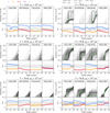 |
Fig. C.1 Same as Fig. 3, but for various complex organic molecules. |
| In the text | |
|
Fig. C.2 Width of the 68.27% confidence intervals of abundances of some complex organic molecules at various temperatures (averaged over all densities) over time at ζ=1.3 × 10⁻¹⁷ s−1 and FUV=1 Habing. The solid, dashed, dotted, dashed-dotted, and densely dotted lines correspond to 10, 20, 30, 40 and 50 K, respectively. The dashed gray line indicates a width of 2 orders of magnitude. |
| In the text | |
|
Fig. D.1 Width of the 68.27% confidence intervals of abundances of selected ice species while only varying the reaction energy barriers at various temperatures (averaged over all densities) over time at ζ=1.3 × 10⁻¹⁷ s−1 and FUV=1 Habing. The solid, dashed, dotted, dashed-dotted, and densely dotted lines correspond to 10, 20, 30, 40 and 50 K, respectively. The dashed gray line indicates a width of 2 orders of magnitude. |
| In the text | |
Current usage metrics show cumulative count of Article Views (full-text article views including HTML views, PDF and ePub downloads, according to the available data) and Abstracts Views on Vision4Press platform.
Data correspond to usage on the plateform after 2015. The current usage metrics is available 48-96 hours after online publication and is updated daily on week days.
Initial download of the metrics may take a while.