| Issue |
A&A
Volume 706, February 2026
|
|
|---|---|---|
| Article Number | A173 | |
| Number of page(s) | 12 | |
| Section | Galactic structure, stellar clusters and populations | |
| DOI | https://doi.org/10.1051/0004-6361/202557992 | |
| Published online | 10 February 2026 | |
APOGEE physical properties of globular cluster tidal tails
1
Instituto Interdisciplinario de Ciencias Básicas (ICB), CONICET-UNCuyo,
Padre J. Contreras 1300,
M5502JMA,
Mendoza,
Argentina
2
Consejo Nacional de Investigaciones Científicas y Técnicas (CONICET),
Godoy Cruz 2290,
C1425FQB,
Buenos Aires,
Argentina
★ Corresponding author: This email address is being protected from spambots. You need JavaScript enabled to view it.
Received:
5
November
2025
Accepted:
12
December
2025
Abstract
A recent model prediction claimed that there is a correlation between the formation scenarios of globular clusters (i.e., whether they formed in situ or in dark matter halos that were accreted into the Milky Way) and some properties of their tidal tails, particularly their widths (w), and their dispersions in the z-component of the angular momentum (σLZ) and in the line-of-sight (σVLOS) and tangential (σVTan) velocities. I exploited the APOGEE DR17 database and selected highly confident tidal tail members of 17 Milky Way globular clusters, for which the above four properties were computed for the first time. From all the possible paired property combinations, I found that σVLos and σVTan resulted as highly correlated, nearly to the identity relationship. This observation-based correlation was in overall very good agreement with that arising from the aforementioned predictions. Additionally, when the four analyzed properties are linked to the accretion groups of the Milky Way with which the globular clusters are meant to be associated, I found kinematically cold and hot tidal tails pertaining to globular clusters distributed in all the considered accretion groups. This outcome could be evidence that globular clusters form in galaxies within a wide variety of dark matter halos, with different masses and profiles.
Key words: methods: data analysis / globular clusters: general
© The Authors 2026
 Open Access article, published by EDP Sciences, under the terms of the Creative Commons Attribution License (https://creativecommons.org/licenses/by/4.0), which permits unrestricted use, distribution, and reproduction in any medium, provided the original work is properly cited.
This article is published in open access under the Subscribe to Open model. This email address is being protected from spambots. You need JavaScript enabled to view it. to support open access publication.
1 Introduction
Recently, Malhan et al. (2021) and Malhan et al. (2022) showed that there is a correspondence between some physical properties of globular cluster tidal tails and the formation environment of the globular clusters, specifically whether they were accreted or formed in situ. In particular, they found that the width of the tidal tails, and the dispersions in the z-component of the angular momentum, and in the line-of-sight and tangential velocities of member stars of globular cluster tidal tails can tell us something about the globular clusters’ origin. They simulated globular clusters formed in a low-mass galaxy halo with cored or cuspy central density profiles of dark matter that later merged with the Milky Way and globular clusters formed in situ. On average, globular clusters from cuspy profiles have tidal tails with dispersion in the z-component of the angular momentum, and in the line-of-sight and tangential velocities that are three times larger than those of clusters formed in cored dark matter profiles. Likewise, globular clusters formed in situ have mean values of dispersion of these properties nearly ten times smaller than those for globular clusters accreted inside cored subhalos. The tidal tail width increases from some tens of parsecs for those formed in situ to a few hundred parsecs for globular clusters formed inside cored dark matter profiles, and to a few kiloparsecs for cuspy ones.
These predictions open, for the first time, the possibility of disentangling the origin of individual globular clusters without the need of constructing a multicomponent model for the whole population of galactic globular clusters (see, e.g., Massari et al. 2019; Forbes 2020; Callingham et al. 2022). However, the usefulness of the predictions depends on the knowledge of the aforementioned quantities for a statistically significant sample of member stars of globular cluster tidal tails. Out of all Milky Way globular clusters with tidal tails (Piatti & Carballo-Bello 2020; Zhang et al. 2022), NGC 288 and NGC 5904 (M5) are the only globular clusters with a tangential velocity dispersion analysis. Piatti (2023) used the 50 highest ranked tidal tail member candidates in M5 (Grillmair 2019) to conclude that the globular cluster formed inside a ~ 109 M⊙ cuspy dark matter subhalo. Likewise, Grillmair (2025) found that NGC 288’s tidal tails are consistent with the cluster being stripped from a parent galaxy with a large cored dark matter halo, which is in very good agreement with the results by Belokurov et al. (2018) and Helmi et al. (2018), who found that it could have been brought into the Milky Way halo during the Gaia-Enceladus-Sausage event.
The Apache Point Observatory Galactic Evolution Experiment (APOGEE; Majewski et al. 2017) gave us the opportunity to exploit a homogeneous chemical composition and kinematics database for a large percentage of the Milky Way globular cluster population, with the aim of computing the width of tidal tails, and the dispersion of the z-component of the angular momentum, and the line-of-sight and tangential velocities of globular cluster tidal tail members. Precisely, the main aim of this work is to probe the performance of the predictions by Malhan et al. (2021) and Malhan et al. (2022) by comparing their outcomes with the observation-based dispersion values of globular clusters with data available in APOGEE. In Section 2, I describe the employed data and the selection of globular cluster tidal tail members, and the computation of the dispersion values of the four mentioned astrophysical properties. I analyze and discuss our findings in Section 3, and in Section 4 I summarize the main conclusions of this work.
2 Data handling
Schiavon et al. (2024) compiled a catalog of 72 Milky Way globular clusters with information of the chemistry (20 species), radial velocities, and the imported Gaia EDR3 data (Gaia Collaboration 2021) of 6422 member stars, retrieved from APOGEE DR17 (Abdurro’uf et al. 2022). The stars contained in the Schiavon et al. (2024) APOGEE value-added catalog are mainly red giants for which the most reliable abundances correspond to C, N, O, Mg, Al, Si, Mn, Fe, and Ni. They defined two types of cluster members, namely likely members and outliers; the likely members are those with the highest probabilities of being cluster members. As a stringent selection criterion, I used here only the likely members, and the abundances of the eight most reliable chemical elements mentioned above, in addition to [Fe/H].
With the aim of extracting from APOGEE DR17 the tidal tail stars of Milky Way globular clusters, I relied on their abundances of chemical elements, which have negligible variations along their lifetimes. Until recently, the mean proper motion and/or radial velocity of globular clusters were used as selection criteria of tidal tail stars, assuming that the tidal tail stars should share the motions of cluster stars (Sollima 2020; Xu et al. 2024). However, since tidal tail stars escape from the cluster, they need to reach velocities different from those of the cluster members. In addition, the Milky Way gravitational field accelerates them differently, so that the mean kinematic properties of tidal tail stars vary along the tail extensions (Piatti et al. 2023; Grondin et al. 2024). Because of the diverse orientation in space of globular cluster tidal tails, the heliocentric distances of their stars vary along the tails, and thus it would not be appropriate to adopt a constant distance for them. This also prevents us from employing color-magnitude diagrams to select tidal tail stars placed along the cluster main sequences, since the ordinate variable of the color-magnitude diagram depends on the star’s heliocentric distance.
I first used the Schiavon et al. (2024)'s APOGEE value-added catalog with the aim of computing the mean values and dispersion of [Fe/H] and those for the other eight chemical elements of the 72 Milky Way globular clusters. Table B.1 lists the resulting values. I did not include Ter 5 because it is a Milky Way bulge globular cluster with a complex formation and evolution history and a remarkable metallicity spread (Origlia et al. 2025). For each globular cluster I then searched the APOGEE DR17 database for stars with chemical element abundance patterns within 1σ of that globular cluster, to be consistent with the definition of likely members of Schiavon et al. (2024) used here; this is a way to make a conservative selection that leads to a very pure sample. This provides a high signal-to-noise ratio for contrasting the tidal tail profiles to the contamination. I retrieved only stars complying with the following:
![Mathematical equation: {\rm [Fe/H]}_{\rm star} - <{\rm [Fe/H]}_{\rm cls} >\, \le \sigma({\rm [Fe/H]}_{\rm cls})](/articles/aa/full_html/2026/02/aa57992-25/aa57992-25-eq1.png)
and
![Mathematical equation: {\rm [X/Fe]}_{\rm star} - <{\rm [X/Fe]}_{\rm cls}> \,\le \sigma({\rm [X/Fe]}_{\rm cls}).](/articles/aa/full_html/2026/02/aa57992-25/aa57992-25-eq2.png)
Here X represent the chemical elements C, N, O, Mg, Al, Si, Mn, and Ni, and the “star” and “cls” subscripts refer to the values of the searched stars in the APOGEE DR17 database and the clusters’ mean values and dispersions in Table B.1. From this search, I found 42 globular clusters with no selected stars and 12 globular clusters with a few stars, which I removed from the final sample. Figure 1 depicts the distribution of the 23 917 finally extracted stars for the 17 surviving globular clusters in the log g versus Teff plane. As can be seen, they are all red giant stars.
The similarity imposed between the chemical element abundance patterns of tidal tail and cluster stars does not warrant that the selected stars are indeed globular cluster tidal tails. As is known, the Milky Way disks and halo are populated by stars with metallicity patterns that are indistinguishable from those of globular clusters (Reddy et al. 2003; Venn et al. 2004; Reddy et al. 2006; Nissen & Schuster 2010). In order to remove any potential star not belonging to globular cluster tidal tails, I required that the selected stars trace a smooth stellar path from the globular cluster’s center, are located beyond the globular cluster’s radius, and show a smooth correlation of their widths and of their z-component of the angular momentum, line-of-sight and tangential velocities with the position along the tidal tails. I relied on this aspect in the recipe outlined by Malhan et al. (2021) and Malhan et al. (2022) to compute the dispersion of different properties along the tidal tails. Briefly, they defined an angular coordinate along the tidal tails and another perpendicular to them. Then they fitted the variation of each considered property along 30° long segments of tidal tails with a smooth polynomial, and subtracted the fitted function from the property values to obtain the residual distribution. The standard deviation of this distribution provides the property dispersion of that tidal tail segment. These criteria were aimed at selecting a coherent sample of stars highly ranked as globular cluster tidal tail members.
For that purpose, I used the globular cluster central coordinates (right ascension, declination), mean heliocentric distances, and radial velocities from Schiavon et al. (2024), and Gaia astrometry information (parallax, proper motion) included into the APOGEE DR17 database (Abdurro’uf et al. 2022), and followed the recipes summarized above (see also, Piatti 2025) to compute the variation in the four considered properties along the physical extension of the tidal tails. In brief, I computed the Cartesian coordinates (X, Y, Z) and space velocity components (VX, VY, V>) of each selected star, and from them I obtained the z-component of their angular momentum. I also calculated their tangential velocities VTan = k × (1/parallax) × μ, where k = 4.7405 km s−1 kpc−1 (mas/yr)−1 and μ is the total proper motion. Then, I carried out two perpendicular rotations around the cluster’s center in order to have the tidal tails centered on the cluster and mainly oriented along one of the three perpendicular axes (ϕ1). First, I rotated the galactic (X′ Y, Z) system around the Y-axis to the (X′ Y, φ3) system as


where θ is the rotating angle, to have the tidal tail in the (X′ Z) plane aligned along the X′ direction. Then, I rotated the (X′, Y, φ3) system around the φ3−axis to the (φ1,φ2, φ3) system, as


where ψ is the rotating angle, to have the tidal tail in the (X′ Y) plane aligned along the φ1 direction. The appropriate rotation angles θ and ψ were obtained by visually inspecting the orientation of the stellar density contours in the rotated 3D coordinate system. I called the rotated framework (φ1, φ2, φ3), where φ1 is along the tidal tails, φ2 is perpendicular to φ1 and contained in the tidal tails plane, and φ3 is perpendicular to φ1 and φ2 . Figure 2 illustrates the projected spatial distribution in the (φ1,φ2) plane of the selected tidal tails stars of NGC 5139. Figure A.1 includes similar figures of the 16 remaining globular clusters, while the source identifications of the selected stars are compiled in Table B.3. The reasons supporting the choice of Cartesian galactocentric coordinates instead of angular ones and the transformation equations of the two perpendicular rotations are described in Piatti (2025).
I then plotted the z-component of the angular momentum (Lz), and the line-of-sight (VLOS) and tangential (VTan) velocities as a function of φ1 for all the selected stars. Figure 3 illustrates the resulting spatial distributions of VLOS, VTan, and Lz along the tidal tail direction (φ1) of NGC 5139. The observed distributions were fitted with polynomials of up to second order, which represent the mean behavior of these parameters along the tails. I visually inspected the fits of the properties of the 17 globular clusters, and they visibly match the ensemble of points. Finally, I calculated the residuals (observed individual value - mean fitted value for the corresponding φ1) and the respective standard dispersion, namely σVLOS, σVTan, and σLZ, which are the properties proposed by Malhan et al. (2021) and Malhan et al. (2022) sensible to the origin of Milky Way globular clusters, i.e., whether formed in situ or in dwarf galaxies with central cored or cuspy dark matter profiles. The tidal tail width (w) was computed by calculating the average diameter of the tidal tail’s dispersion in the (φ2,φ3) plane. The uncertainties in these quantities are based on the errors in parallax, proper motions, and radial velocity. I generated random kicks proportional to the error, which means that I sampled from the actual measurement from the uniform distribution within the interval [measurement - error, measurement + error]. I randomly generated a thousand different values of parallax, proper motions, and radial velocity based on their errors (variable = mean_value + variable_error×2×(0.5 - t), with −1<t<1 randomly chosen), and repeated the computation of all the quantities following the procedure described above. I used all the 1000 different w, σVLOS, σVTan, and σLZ values to calculate their mean and dispersion. I checked that by using subsamples of 100 values it resulted in a negligible mean and dispersion with respect to whole sample. Table B.2 lists the resulting w, σVLOS, σVTan, and σLZ values for 17 Milky Way globular clusters. Its second column shows the length of the tidal tails, calculated as the difference in φ1 between the two farthest stars located on opposite sides from the cluster’s center. The resulting σVTan value of NGC 5904 is in very good agreement with that derived by Piatti (2023, 7.50±1.38 km/s) using the tangential velocities of 50 highly ranked tidal tail members.
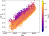 |
Fig. 1 log g vs. Teff plane with all the stars retrieved from the APOGEE DR17 database (see text for details). |
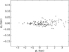 |
Fig. 2 Spatial diatribution in the (φ1,φ2) plane (see Piatti 2025) of selected tidal tail stars of NGC 5139. |
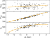 |
Fig. 3 VLOS (km/s), VTan (km/s), and Lz (km/s kpc) as a function of φ1 for selected tidal tail stars of NGC 5139 (black dots). The orange line is the best-fit polynomial. |
3 Analysis and discussion
As far as I am aware, Table B.2 is the largest compilation of globular cluster tidal tails with their widths, and dispersion in the z-component of the angular momentum, and in the line-of-sight and tangential velocities derived from observational data of selected members. Therefore, it represents a valuable data set to explore whether there is any correlation between these properties, how well they match the models of Malhan et al. (2021) and Malhan et al. (2022), and what they tell us about the association of the globular clusters with the different accretion groups of the Milky Way (e.g., Callingham et al. 2022). Furthermore, it can help in disentangling whether these parameters are drivers of the globular clusters’ origin, and also to show the pace of any eventual trends. For these reasons, I started by digging into the relationships of each of these parameters with respect to the three remaining parameters.
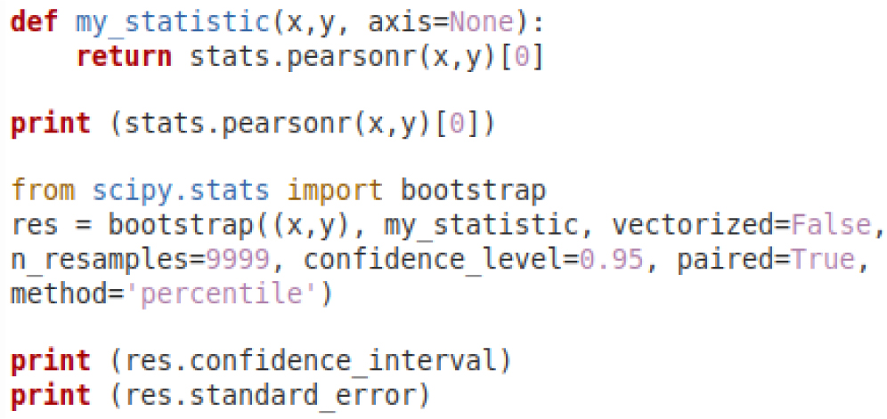
Figure 4 depicts the collection of all the attempted relationships. At first glance, σVLOS and σVTan seem to be tightly correlated; σLz shows a mild linear correlation with both velocity dispersions, while w does not seem to show any robust trend with any of the other parameters. In order to quantify the visually suggested behaviors, I have computed bootstrap confidence intervals for two different statistics, namely the Pearson and Spearman correlations, and the resulting values are shown in Table 1, which confirms the suggested trends. The confidence intervals were computed using scipy.stats.bootstrap1. For the sake of clarity, an example is provided below.
These outcomes show that the physical width of tidal tails would not be necessarily linked with their kinematic agitation, in the sense that the kinematically hotter a tidal tail (σ > 1-2 km/s), the wider its extension, as expected. Although some indication that the latter could be true, the tidal tails sample analyzed here could be hampering such a trend. Nevertheless, the present results also allow for the possibility that some hot tidal tails (σ > 5 km/s) are relatively thin (w < 300 pc).
From a purely kinematic point of view, it would seem that the tidal tails are similarly agitated in any observed direction, as judged by the nearly identity relationship found between the dispersion of perpendicular velocities (VLOS versus VTan). Whenever a physical position parameter is combined with the kinematic behavior, as is the case of Lz, some scattered points appear in the dispersion plot (σVLOS,σVTan vs. σLz diagrams). If we discarded these few points, a clearer linear relation between the properties involved would arise. Since σvLOS and σvTan are well correlated, the scattered points in the σVLOS,σVTan versus σLz planes should be due to σLz. I have checked the fits of Lz as a function of φ1 for these scatted points (NGC 1851, NGC 1904) and found a well-fitted function with points slightly departing from the mean fitted relationship. This means that σLz cannot be smaller as required for a better linear behavior with σVLOS and σVTan, respectively.
The simulations carried out by Malhan et al. (2021) and Malhan et al. (2022) predicted that globular clusters formed in situ, or in dark matter subhalos with cored and cuspy profiles that were accreted into the Milky Way, develop tidal tails with increasing width, and dispersion of the z-component of the angular momentum and of the line-of-sight and tangential velocities, respectively. I superimposed the range of values of these properties obtained by Malhan et al. (2021) and Malhan et al. (2022) on the observation-based results illustrated in Figure 4. Figure 5 shows the resulting comparison, where probability distribution functions of globular clusters formed in situ, in 108 M⊙ and 109 M⊙ dark matter halos with cored and cuspy profiles are shown in magenta, blue, yellow, orange, and red, respectively.
The simulated properties show steady increasing relationships for all the examined 2D planes. The values of the four properties for the 109 M⊙ cuspy profiles are notably the largest ones, while some superposition exits in σVLOS and σVTan between the 109 M⊙ cored profile and the in situ 108 M⊙ cored and 108 M⊙ cuspy profiles, respectively. This implies that σVLOS and σVTan cannot unambiguously point to a unique globular cluster formation scenario, as seems to be the case of the simulated w and σLz values. Nevertheless, because of the overall monotonic behavior of any paired properties seen in Figure 4 and in Figure 5, the present observation-based results bring support to the predicted different origins of globular clusters.
A closer look at Figure 5 reveals that, for each panel, the slopes in the observation-based and in the simulated relations are in reasonably good agreement for the σVTan - σVLos and the σLz−w planes, while they depart significantly when σLz and w are plotted against σVLOS or σLz. The reason for such a difference could be due to the predicted much larger values of w and σLz for the 109 M⊙ cuspy model, even though the 108 M⊙ cuspy profile also shows some slightly larger w and σLz values. From these behaviors, it would seem to be recommendable to employ the σVLOS versus σVTan plane to infer the origins of globular clusters. I would like to note that disentangling in the simulations what is causing the split from the observation-based trends could become a complex analysis of assumptions, different employed parameters, computational details that are beyond of this work. Indeed, models of globular cluster tidal tails based on different physical considerations computed by Grondin et al. (2024) produce different w, σLz, σVLOS, and σVTan relations (Piatti 2025).
Finally, I linked the properties of globular cluster tidal tails from Table B.2 with the accretion group of the Milky Way associated with that globular cluster proposed by Callingham et al. (2022). From the defined accretion groups, the presently studied globular clusters belong to the Milky Way disk, Sequoia (Seq), Helmi, Kraken, Gaia-Enceladus-Sausage (GES), or Sagittarius (Sag). Figure 6 shows the ranges of the parameter values for these accretion groups. As can be seen, the tidal tails of the globular clusters formed in situ or in an accreted galaxy can be kinematically cold or hot (σ < or > ~2 km/s). Bearing in mind the different formation scenarios of globular clusters proposed by Malhan et al. (2021) and Malhan et al. (2021), this implies that the population of globular clusters of a galaxy can form within a variety of dark matter halos, in terms of mass and profiles. This would also seem valid for globular clusters formed in situ. In addition to this overall characteristic, Figure 6 also tells us that NGC 6715, the nuclear globular cluster of Sagittarius, has the widest and the kinematically hottest tidal tails. Despite the limited number of globular clusters analyzed, Figure 6 would still seem to suggest that subtle differences in the ranges of w, σVLOS, and σVTan, and σLz exist among the different accretion groups of the Milky Way.
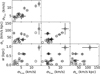 |
Fig. 4 Correlation between different globular cluster tidal tail properties using the information in Table B.2. |
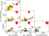 |
Fig. 5 Same as Figure 4 with the predictions from Malhan et al. (2021) and Malhan et al. (2021) superimposed. The different colors refer to globular clusters formed in situ (magenta), in 108 M⊙ and 109 M⊙ cored profiles (blue and yellow, respectively), and in 108 M⊙ and 109 M⊙ cuspy profiles (orange and red, respectively). |
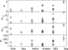 |
Fig. 6 w (kpc), VLOS (km/s), VTan (km/s), and Lz (km/s kpc) as a function of different accretion groups of the Milky Way, according to Callingham et al. (2022) Shown from left to right are the Milky Way disk, Sequoia (Seq), Helmi, Kraken, Gaia-Enceladus-Sausage (GES), and Sagittarius (Sag). |
4 Conclusions
In this study, I explored from an observation-based point of view the scope of the predictions by Malhan et al. (2021) and Malhan et al. (2022) with respect to the relation claimed between the origin of globular clusters and the range of values of some properties of their tidal tails. I specifically looked at their widths, and their dispersion in the z-component of the angular momentum, and in the line-of-sight and tangential velocities. I took advantage of the APOGEE DR17 database in conjunction with the APOGEE value-added catalog of globular clusters to compile the largest data set of the four properties mentioned above of globular cluster tidal tails. They were computed following the recipe outlines in Malhan et al. (2021). Then, from an in-depth analysis of these properties for 17 globular clusters, the following conclusions are drawn:
σVLOS and σVTan were found to be tightly correlated; correlations involving σLz show a mild linear relationship, while those with w do not seem to show a robust trend. However, the latter could be blurred by a number of scattered points. The nearly identity relationship between σVLOS and σVTan reveals that, along the tidal tails, there is not any preferred direction of kinematic agitation. By comparing the resulting trends with those coming from the probability distribution functions obtained from the simulations carried out by Malhan et al. (2021) and Malhan et al. (2022), I found an overall agreement, which brings support to their predictions that globular clusters formed in situ or in dark matter halos with cored or cuspy profiles that were accreted into the Milky Way span different ranges of values of the four mentioned properties.
Because larger values of w and σLz for dark matter halos with cuspy profiles are predicted by the simulations in comparison with the observation-based ones obtained here, the σVLOS versus σVTan plane would seem to be more suitable to infer the origin of globular clusters. Nevertheless, the latter diagram shows some superposition between the probability distribution function of the 109 M⊙ cored dark matter profile with those of in situ, 108 M⊙ cored, and 108 M⊙ cuspy profiles, respectively.
When the values of the four analyzed properties are linked to the accretion groups of the Milky Way with which globular clusters are associated, I found kinematically cold and hot globular tidal tails belonging to globular clusters distributed in almost all the considered groups, namely: the Milky Way disk, Sequoia, Helmi, Kraken, Gaia-Enceladus-Sausage, and Sagittarius. From the perspective of the formation scenario of globular clusters, and in the context of Malhan et al. (2021)'s predictions, this outcome is observational evidence that globular clusters can form within a variety of dark matter halos in terms of mass and profiles.
Acknowledgements
I thank K. Malhan for his kind exchange of ideas. I thank the referee for the thorough reading of the manuscript and timely suggestions to improve it. Data for reproducing the figures and analysis in this work are available upon request to the first author.
References
- Abdurro’uf Accetta, K., Aerts, C., et al. 2022, ApJS, 259, 35 [NASA ADS] [CrossRef] [Google Scholar]
- Belokurov, V., Erkal, D., Evans, N. W., Koposov, S. E., & Deason, A. J. 2018, MNRAS, 478, 611 [Google Scholar]
- Callingham, T. M., Cautun, M., Deason, A. J., et al. 2022, MNRAS, 513, 4107 [NASA ADS] [CrossRef] [Google Scholar]
- Forbes, D. A. 2020, MNRAS, 493, 847 [Google Scholar]
- Gaia Collaboration (Brown, A. G. A., et al.) 2021, A&A, 649, A1 [NASA ADS] [CrossRef] [EDP Sciences] [Google Scholar]
- Grillmair, C. J. 2019, ApJ, 884, 174 [Google Scholar]
- Grillmair, C. J. 2025, ApJ, 979, 75 [Google Scholar]
- Grondin, S. M., Webb, J. J., Lane, J. M. M., Speagle, J. S., & Leigh, N. W. C. 2024, MNRAS, 528, 5189 [Google Scholar]
- Helmi, A., Babusiaux, C., Koppelman, H. H., et al. 2018, Nature, 563, 85 [Google Scholar]
- Majewski, S. R., Schiavon, R. P., Frinchaboy, P. M., et al. 2017, AJ, 154, 94 [NASA ADS] [CrossRef] [Google Scholar]
- Malhan, K., Valluri, M., & Freese, K. 2021, MNRAS, 501, 179 [Google Scholar]
- Malhan, K., Valluri, M., Freese, K., & Ibata, R. A. 2022, ApJ, 941, L38 [Google Scholar]
- Massari, D., Koppelman, H. H., & Helmi, A. 2019, A&A, 630, L4 [NASA ADS] [CrossRef] [EDP Sciences] [Google Scholar]
- Nissen, P. E., & Schuster, W. J. 2010, A&A, 511, L10 [NASA ADS] [CrossRef] [EDP Sciences] [Google Scholar]
- Origlia, L., Ferraro, F. R., Fanelli, C., et al. 2025, A&A, 697, A19 [NASA ADS] [CrossRef] [EDP Sciences] [Google Scholar]
- Piatti, A. E. 2023, MNRAS, 525, L72 [Google Scholar]
- Piatti, A. E. 2025, ApJ, 983, 123 [Google Scholar]
- Piatti, A. E., & Carballo-Bello, J. A. 2020, A&A, 637, L2 [NASA ADS] [CrossRef] [EDP Sciences] [Google Scholar]
- Piatti, A. E., Illesca, D. M. F., Massara, A. A., et al. 2023, MNRAS, 518, 6216 [Google Scholar]
- Reddy, B. E., Tomkin, J., Lambert, D. L., & Allende Prieto, C. 2003, MNRAS, 340, 304 [Google Scholar]
- Reddy, B. E., Lambert, D. L., & Allende Prieto, C. 2006, VizieR Online Data Catalog: Elemental abundances for 176 stars (Reddy+, 2006), VizieR On-line Data Catalog: J/MNRAS/367/1329. Originally published in: 2006MNRAS.367.1329R [Google Scholar]
- Schiavon, R. P., Phillips, S. G., Myers, N., et al. 2024, MNRAS, 528, 1393 [CrossRef] [Google Scholar]
- Sollima, A. 2020, MNRAS, 495, 2222 [Google Scholar]
- Venn, K. A., Irwin, M., Shetrone, M. D., et al. 2004, AJ, 128, 1177 [NASA ADS] [CrossRef] [Google Scholar]
- Xu, C., Tang, B., Li, C., et al. 2024, A&A, 684, A205 [NASA ADS] [CrossRef] [EDP Sciences] [Google Scholar]
- Zhang, S., Mackey, D., & Da Costa, G. S. 2022, MNRAS, 513, 3136 [NASA ADS] [CrossRef] [Google Scholar]
Appendix A Selected globular clusters’ stars
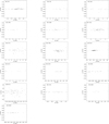 |
Fig. A.1 Spatial distribution in the (φ1,φ2) plane (see Piatti 2025) of selected tidal tail stars. |
Appendix B Mean properties of Milky Way globular clusters in the Schiavon et al. (2024) APOGEE added-value catalog
Mean abundances of chemical elements in Milky Way globular clusters.
σVLOS, σVTan, and σLz values of Milky Way globular clusters.
Source_ID from APOGEE DR17 of selected stars of globular clusters.
All Tables
All Figures
|
Fig. 1 log g vs. Teff plane with all the stars retrieved from the APOGEE DR17 database (see text for details). |
| In the text | |
|
Fig. 2 Spatial diatribution in the (φ1,φ2) plane (see Piatti 2025) of selected tidal tail stars of NGC 5139. |
| In the text | |
|
Fig. 3 VLOS (km/s), VTan (km/s), and Lz (km/s kpc) as a function of φ1 for selected tidal tail stars of NGC 5139 (black dots). The orange line is the best-fit polynomial. |
| In the text | |
|
Fig. 4 Correlation between different globular cluster tidal tail properties using the information in Table B.2. |
| In the text | |
|
Fig. 5 Same as Figure 4 with the predictions from Malhan et al. (2021) and Malhan et al. (2021) superimposed. The different colors refer to globular clusters formed in situ (magenta), in 108 M⊙ and 109 M⊙ cored profiles (blue and yellow, respectively), and in 108 M⊙ and 109 M⊙ cuspy profiles (orange and red, respectively). |
| In the text | |
|
Fig. 6 w (kpc), VLOS (km/s), VTan (km/s), and Lz (km/s kpc) as a function of different accretion groups of the Milky Way, according to Callingham et al. (2022) Shown from left to right are the Milky Way disk, Sequoia (Seq), Helmi, Kraken, Gaia-Enceladus-Sausage (GES), and Sagittarius (Sag). |
| In the text | |
|
Fig. A.1 Spatial distribution in the (φ1,φ2) plane (see Piatti 2025) of selected tidal tail stars. |
| In the text | |
Current usage metrics show cumulative count of Article Views (full-text article views including HTML views, PDF and ePub downloads, according to the available data) and Abstracts Views on Vision4Press platform.
Data correspond to usage on the plateform after 2015. The current usage metrics is available 48-96 hours after online publication and is updated daily on week days.
Initial download of the metrics may take a while.