| Issue |
A&A
Volume 707, March 2026
|
|
|---|---|---|
| Article Number | A176 | |
| Number of page(s) | 20 | |
| Section | Cosmology (including clusters of galaxies) | |
| DOI | https://doi.org/10.1051/0004-6361/202348713 | |
| Published online | 06 March 2026 | |
Euclid: Constraints on f(R) cosmologies from the spectroscopic and photometric primary probes★
1
Institute for Theoretical Particle Physics and Cosmology (TTK), RWTH Aachen University 52056 Aachen, Germany
2
INAF-Osservatorio Astronomico di Roma Via Frascati 33 00078 Monteporzio Catone, Italy
3
INFN-Sezione di Roma, Piazzale Aldo Moro, 2 – c/o Dipartimento di Fisica Edificio G. Marconi 00185 Roma, Italy
4
Departamento de Física, FCFM, Universidad de Chile Blanco Encalada 2008 Santiago, Chile
5
Department of Physics “E. Pancini”, University Federico II Via Cinthia 6 80126 Napoli, Italy
6
Dipartimento di Fisica, Università degli Studi di Torino Via P. Giuria 1 10125 Torino, Italy
7
INFN-Sezione di Torino Via P. Giuria 1 10125 Torino, Italy
8
INAF-Osservatorio Astrofisico di Torino Via Osservatorio 20 10025 Pino Torinese (TO), Italy
9
Dipartimento di Fisica, Università degli studi di Genova, and INFN-Sezione di Genova Via Dodecaneso 33 16146 Genova, Italy
10
INAF-Osservatorio Astronomico di Trieste Via G. B. Tiepolo 11 34143 Trieste, Italy
11
SISSA, International School for Advanced Studies Via Bonomea 265 34136 Trieste TS, Italy
12
IFPU, Institute for Fundamental Physics of the Universe Via Beirut 2 34151 Trieste, Italy
13
Dipartimento di Fisica “Aldo Pontremoli”, Università degli Studi di Milano Via Celoria 16 20133 Milano, Italy
14
INFN-Sezione di Milano Via Celoria 16 20133 Milano, Italy
15
Institute of Cosmology and Gravitation, University of Portsmouth Portsmouth PO1 3FX, UK
16
Institut de Recherche en Astrophysique et Planétologie (IRAP), Université de Toulouse, CNRS, UPS, CNES 14 Av. Edouard Belin 31400 Toulouse, France
17
Université de Genève, Département de Physique Théorique and Centre for Astroparticle Physics 24 quai Ernest-Ansermet CH-1211 Genève 4, Switzerland
18
Institute of Space Sciences (ICE, CSIC), Campus UAB, Carrer de Can Magrans s/n 08193 Barcelona, Spain
19
Institut d’Estudis Espacials de Catalunya (IEEC), Edifici RDIT, Campus UPC 08860 Castelldefels Barcelona, Spain
20
Université Paris-Saclay, Université Paris Cité, CEA, CNRS, AIM 91191 Gif-sur-Yvette, France
21
Institut für Theoretische Physik, University of Heidelberg Philosophenweg 16 69120 Heidelberg, Germany
22
Université St Joseph; Faculty of Sciences Beirut, Lebanon
23
Institute Lorentz, Leiden University Niels Bohrweg 2 2333 CA Leiden, The Netherlands
24
Dipartimento di Scienze Matematiche, Fisiche e Informatiche, Università di Parma Viale delle Scienze 7/A 43124 Parma, Italy
25
INFN Gruppo Collegato di Parma Viale delle Scienze 7/A 43124 Parma, Italy
26
Institut de Physique Théorique, CEA, CNRS, Université Paris-Saclay 91191 Gif-sur-Yvette Cedex, France
27
Aix-Marseille Université, CNRS/IN2P3, CPPM Marseille, France
28
Mullard Space Science Laboratory, University College London Holmbury St Mary Dorking Surrey RH5 6NT, UK
29
Institute for Astronomy, University of Edinburgh, Royal Observatory Blackford Hill Edinburgh EH9 3HJ, UK
30
Higgs Centre for Theoretical Physics, School of Physics and Astronomy, The University of Edinburgh Edinburgh EH9 3FD, UK
31
Université Paris-Saclay, CNRS, Institut d’astrophysique spatiale 91405 Orsay, France
32
INAF-IASF Milano Via Alfonso Corti 12 20133 Milano, Italy
33
Instituto de Física Teórica UAM-CSIC, Campus de Cantoblanco 28049 Madrid, Spain
34
ESAC/ESA, Camino Bajo del Castillo, s/n. Urb. Villafranca del Castillo 28692 Villanueva de la Cañada Madrid, Spain
35
INAF-Osservatorio di Astrofisica e Scienza dello Spazio di Bologna Via Piero Gobetti 93/3 40129 Bologna, Italy
36
Dipartimento di Fisica e Astronomia, Università di Bologna Via Gobetti 93/2 40129 Bologna, Italy
37
INFN-Sezione di Bologna Viale Berti Pichat 6/2 40127 Bologna, Italy
38
Max Planck Institute for Extraterrestrial Physics Giessenbachstr. 1 85748 Garching, Germany
39
Dipartimento di Fisica, Università di Genova Via Dodecaneso 33 16146 Genova, Italy
40
INFN-Sezione di Genova Via Dodecaneso 33 16146 Genova, Italy
41
INAF-Osservatorio Astronomico di Capodimonte Via Moiariello 16 80131 Napoli, Italy
42
Instituto de Astrofísica e Ciências do Espaço, Universidade do Porto, CAUP Rua das Estrelas PT4150-762 Porto, Portugal
43
Institut de Física d’Altes Energies (IFAE), The Barcelona Institute of Science and Technology, Campus UAB 08193 Bellaterra (Barcelona), Spain
44
Port d’Informació Científica, Campus UAB C. Albareda s/n 08193 Bellaterra (Barcelona), Spain
45
INFN section of Naples Via Cinthia 6 80126 Napoli, Italy
46
Dipartimento di Fisica e Astronomia “Augusto Righi” – Alma Mater Studiorum Università di Bologna Viale Berti Pichat 6/2 40127 Bologna, Italy
47
Centre National d’Etudes Spatiales – Centre spatial de Toulouse 18 avenue Edouard Belin 31401 Toulouse Cedex 9, France
48
Institut national de physique nucléaire et de physique des particules 3 rue Michel-Ange 75794 Paris Cédex 16, France
49
Jodrell Bank Centre for Astrophysics, Department of Physics and Astronomy, University of Manchester Oxford Road Manchester M13 9PL, UK
50
European Space Agency/ESRIN, Largo Galileo Galilei 1 00044 Frascati Roma, Italy
51
Université Claude Bernard Lyon 1, CNRS/IN2P3, IP2I Lyon, UMR 5822 Villeurbanne F-69100, France
52
Institute of Physics, Laboratory of Astrophysics, Ecole Polytechnique Fédérale de Lausanne (EPFL), Observatoire de Sauverny 1290 Versoix, Switzerland
53
UCB Lyon 1, CNRS/IN2P3, IUF, IP2I Lyon 4 rue Enrico Fermi 69622 Villeurbanne, France
54
Departamento de Física, Faculdade de Ciências, Universidade de Lisboa, Edifício C8 Campo Grande PT1749-016 Lisboa, Portugal
55
Instituto de Astrofísica e Ciências do Espaço, Faculdade de Ciências, Universidade de Lisboa, Campo Grande 1749-016 Lisboa, Portugal
56
Department of Astronomy, University of Geneva ch. d’Ecogia 16 1290 Versoix, Switzerland
57
Department of Physics, Oxford University Keble Road Oxford OX1 3RH, UK
58
INFN-Padova Via Marzolo 8 35131 Padova, Italy
59
INAF-Osservatorio Astronomico di Padova Via dell’Osservatorio 5 35122 Padova, Italy
60
Universitäts-Sternwarte München, Fakultät für Physik, Ludwig-Maximilians-Universität München Scheinerstrasse 1 81679 München, Germany
61
INAF-Osservatorio Astronomico di Brera Via Brera 28 20122 Milano, Italy
62
Institute of Theoretical Astrophysics, University of Oslo P.O. Box 1029 Blindern 0315 Oslo, Norway
63
von Hoerner & Sulger GmbH Schlossplatz 8 68723 Schwetzingen, Germany
64
Technical University of Denmark Elektrovej 327 2800 Kgs. Lyngby, Denmark
65
Cosmic Dawn Center (DAWN), Denmark
66
Institut d’Astrophysique de Paris, UMR 7095, CNRS, and Sorbonne Université 98 bis boulevard Arago 75014 Paris, France
67
Max-Planck-Institut für Astronomie Königstuhl 17 69117 Heidelberg, Germany
68
Jet Propulsion Laboratory, California Institute of Technology 4800 Oak Grove Drive Pasadena CA 91109, USA
69
Department of Physics P.O. Box 64 00014 University of Helsinki, Finland
70
Helsinki Institute of Physics, Gustaf Hällströmin katu 2, University of Helsinki Helsinki, Finland
71
NOVA optical infrared instrumentation group at ASTRON Oude Hoogeveensedijk 4 7991PD Dwingeloo, The Netherlands
72
Universität Bonn, Argelander-Institut für Astronomie Auf dem Hügel 71 53121 Bonn, Germany
73
Dipartimento di Fisica e Astronomia “Augusto Righi” – Alma Mater Studiorum Università di Bologna Via Piero Gobetti 93/2 40129 Bologna, Italy
74
Department of Physics, Institute for Computational Cosmology, Durham University South Road Durham DH1 3LE, UK
75
European Space Agency/ESTEC Keplerlaan 1 2201 AZ Noordwijk, The Netherlands
76
Department of Physics and Astronomy, University of Aarhus Ny Munkegade 120 DK-8000 Aarhus C, Denmark
77
Waterloo Centre for Astrophysics, University of Waterloo Waterloo Ontario N2L 3G1, Canada
78
Department of Physics and Astronomy, University of Waterloo Waterloo Ontario N2L 3G1, Canada
79
Perimeter Institute for Theoretical Physics Waterloo Ontario N2L 2Y5, Canada
80
Space Science Data Center, Italian Space Agency Via del Politecnico snc 00133 Roma, Italy
81
Institute of Space Science, Str. Atomistilor nr. 409 Măgurele Ilfov 077125, Romania
82
Dipartimento di Fisica e Astronomia “G. Galilei”, Università di Padova Via Marzolo 8 35131 Padova, Italy
83
Satlantis, University Science Park Sede Bld 48940 Leioa-Bilbao, Spain
84
Aix-Marseille Université, CNRS, CNES, LAM Marseille, France
85
Centro de Investigaciones Energéticas, Medioambientales y Tecnológicas (CIEMAT) Avenida Complutense 40 28040 Madrid, Spain
86
Instituto de Astrofísica e Ciências do Espaço, Faculdade de Ciências, Universidade de Lisboa Tapada da Ajuda 1349-018 Lisboa, Portugal
87
Universidad Politécnica de Cartagena, Departamento de Electrónica y Tecnología de Computadoras Plaza del Hospital 1 30202 Cartagena, Spain
88
Kapteyn Astronomical Institute, University of Groningen PO Box 800 9700 AV Groningen, The Netherlands
89
INFN-Bologna Via Irnerio 46 40126 Bologna, Italy
90
Infrared Processing and Analysis Center, California Institute of Technology Pasadena CA 91125, USA
91
CEA Saclay, DFR/IRFU, Service d’Astrophysique Bat. 709 91191 Gif-sur-Yvette, France
92
Institut d’Astrophysique de Paris 98bis Boulevard Arago 75014 Paris, France
93
ICL, Junia, Université Catholique de Lille, LITL 59000 Lille, France
★★ Corresponding author: This email address is being protected from spambots. You need JavaScript enabled to view it.
Received:
23
November
2023
Accepted:
5
May
2025
Abstract
We forecast the constraints that the Euclid mission will place on the Hu–Sawicki f(R) modified gravity model using galaxy clustering and weak lensing observations. Euclid’s primary probes will provide spectroscopic redshifts, photometric angular clustering, and weak lensing cosmic shear, thus allowing for precise tests of deviations from general relativity. We consider these observables to evaluate how well Euclid can constrain the extended model parameter fR0. For a fiducial value of |fR0| = 5 × 10⁻⁶, we find that in our baseline pessimistic setting, Euclid will constrain log10|fR0| at the 4% level with spectroscopic clustering, at 2.7% with the cross-correlation of photometric probes, and at 1.8% when combining all primary probes. This corresponds to an estimation on this model parameter of approximately |fR0 = (5.0+1.2−0.9 × 10⁻⁶ at the 1σ level. We also forecast constraints for models with |fR0| = 5 × 10⁻⁵ and |fR0| = 5 × 10⁻⁷, finding that Euclid will distinguish these from the standard cosmological model at more than 3σ when using the full combination of primary probes. Euclid will be a powerful experiment to test modifications to gravity, provided that the theoretical systematics of the non-linear modelling are kept under control.
Key words: cosmological parameters / cosmology: observations / cosmology: theory / dark energy / large-scale structure of Universe
This paper is published on behalf of the Euclid Consortium.
Deceased.
© The Authors 2026
 Open Access article, published by EDP Sciences, under the terms of the Creative Commons Attribution License (https://creativecommons.org/licenses/by/4.0), which permits unrestricted use, distribution, and reproduction in any medium, provided the original work is properly cited.
This article is published in open access under the Subscribe to Open model. This email address is being protected from spambots. You need JavaScript enabled to view it. to support open access publication.
1. Introduction
The origin of the accelerated expansion of the Universe continues to challenge our understanding of late-time cosmology. A cosmological constant, Λ, remains in agreement with current data, but its value, when considered as vacuum energy, does not correspond to theoretical predictions and is rather considered as a phenomenological parameter that fits the data. An appealing proposal for an alternative model is that of modifying gravitational interactions felt by particles, either in a universal (the same interaction for all particles) or non-universal way (acting differently on different particles). In this paper, we investigate one popular scenario that belongs to the first class, in which the theory of general relativity (GR) is modified by extending the Ricci scalar, R, in the Hilbert-Einstein action with a general function of it, R → R + f(R). We forecast how well the forthcoming Euclid satellite will constrain this scenario using galaxy clustering (GC), both photometric (GCph) and spectroscopic (GCsp); weak lensing (WL); and their combinations, either photometric probes alone (XCph) or all observables together. In particular, we produce for the first time validated forecasts on the Hu–Sawicki f(R) model (Hu & Sawicki 2007), whose background expansion mimics that of a cosmological constant model while differing at the level of cosmological perturbations. The growth of structure is driven here by a modification of gravity (MG).
Euclid1 is a European Space Agency medium-class space mission launched successfully on July 1, 2023. It carries on board a near-infrared spectrometer and photometer (NISP) (Euclid Collaboration: Jahnke et al. 2025; Euclid Collaboration: Hormuth et al. 2025) and a high-fidelity visible instrument (Euclid Collaboration: Cropper et al. 2025) that will allow it to perform both a spectroscopic and a photometric survey of about 14 000 deg2 of extragalactic sky up to redshifts of about z ≈ 2 (Laureijs et al. 2011; Euclid Collaboration: Scaramella et al. 2022). This survey is known as the Euclid Wide Survey. The main aim of the mission is to measure the geometry of the Universe and the growth of structures to determine the elusive nature of dark matter and dark energy.
Euclid will include a photometric survey measuring positions and shapes of more than a billion galaxies, enabling the analysis of WL and GCph. Given the relatively large redshift uncertainties that we expect from photometric measurements (compared to spectroscopic observations), these analyses will be performed via a tomographic approach, in which galaxies are binned into redshift slices that are considered as 2D (projected) data sets. On the other hand, the spectroscopic survey will provide very precise radial measurements of the position of galaxies. Even if the number density will be lower – compared to the photometric survey – it will allow us to perform a galaxy clustering analysis in three dimensions (GCsp, see Euclid Collaboration: Mellier et al. 2025). The combination of photometric and spectroscopic surveys will enable a powerful test of the two independent gravitational potentials that are predicted to be different within f(R) cosmologies.
We want to quantify the effect of combining the complementary information obtained from the two probes. Euclid Collaboration: Blanchard et al. (2020, EC19 hereafter) have shown that combining GCph and its cross-correlation (XCph) with WL is able to improve the figure of merit by a factor of three for dynamical dark energy models. Our goal here is to explore the impact of cross-correlation on the additional parameter fR0 ≡ df/dR (z = 0) describing the standard model extensions within the f(R) model, which are defined in the next section.
Several studies have tried to constrain the Hu–Sawicki model. Among them, Hu et al. (2016) used Planck15 cosmic microwave background (CMB) data; baryon acoustic oscillations (BAOs); and supernovae Ia from JLA, WiggleZ, and CFHTLenS data sets. They obtained an upper bound of |fR0|< 6.3 × 10⁻⁴ at the 95% confidence level. Similar constraints from cosmological data were obtained, for instance, in Nunes et al. (2017), Okada et al. (2013) and Pérez-Romero & Nesseris (2018). A review of local and astrophysical constraints on fR0 is given by Lombriser (2014). Notably, a bound of |fR0|< 10−6 can be obtained when assuming that the Milky Way can be treated as an isolated system in the cosmological background without environmental screening. Under similar assumptions, astrophysical tests are capable of constraining |fR0| at the level of 10−7 (Baker et al. 2021). Furthermore, Desmond & Ferreira (2020) constrained |fR0|< 1.4 × 10⁻⁸ using galaxy morphology.
After reviewing the f(R) formalism in Sect. 2, we present in Sect. 3 the Euclid primary probes: WL, GCph, and XCph, for the photometric part and GCsp for the spectroscopic part. We then present the survey specifications and analysis scheme in Sect. 4. Finally, we present our results for the fiducial models considered in Sect. 5 and conclude in Sect. 6.
2. Hu–Sawicki f(R) gravity
A modification of Einstein’s theory of GR can be obtained by promoting the linear dependence of the Hilbert-Einstein action, S, on the Ricci scalar, R, to a non-linear function, R + f(R) (Buchdahl 1970):
![Mathematical equation: $$ \begin{aligned} S = \frac{c^4}{16\pi G_{{\scriptscriptstyle \mathrm N}}} \int {\mathrm{d} ^4 x \sqrt{-g} \left[R+f(R)\right]} \,, \end{aligned} $$](/articles/aa/full_html/2026/03/aa48713-23/aa48713-23-eq2.gif) (1)
(1)
where gμν is the metric tensor and GontN is Newton’s gravitational constant. We have expressed explicitly the speed of light, c, to allow for consistency with the choice of units in the observable quantities below.
The f(R) family of cosmologies implies a universal coupling with all matter species, inducing an additional ‘fifth force’. Therefore, an important attribute that a viable late-time f(R) modification must possess to leave a detectable signature in the cosmic structure formation while complying with stringent constraints on gravity in the Solar System is that the functional form f(R) gives rise to a screening mechanism, the so-called ‘chameleon mechanism’ (Khoury & Weltman 2004).
The fifth force has a range determined by the Compton wavelength λontC which has a very direct relationship to the parameter fR0. For cosmological densities one has  Mpc (Hu & Sawicki 2007; Cabre et al. 2012). This relation is important because it is the screening scale that prevents us from having fR0 = 0 as the fiducial model and thus being able to predict the minimum detectable fR0.
As a specific example of this class of theories, we consider here the model proposed by Hu & Sawicki (2007). The functional form of f(R), adopting n = 1 for simplicity and the limit |fR|≪1, is given by
 (2)
(2)
where fR0 < 0,  denotes the Ricci scalar in the cosmological background today, H0 is the Hubble constant, and ΩDE, 0 is the current fractional energy density attributed to a cosmological constant. The only additional free parameter of the model over ΛCDM is therefore fR0.
For the |fR0|≪1 values of interest here, the background expansion history approximates that of ΛCDM and
 (3)
(3)
with the matter energy density parameter Ωm, 0 = 1 − ΩDE, 0. The model parameter |fR0| characterises the magnitude of the deviation from ΛCDM, with smaller |fR0| values corresponding to weaker departures from GR. ΛCDM is recovered in the limit of fR0 → 0.
In general, the background expansion history differs from that of the ΛCDM model, but as shown in Basilakos et al. (2013), deviations are very small and the full history can be described by a series expansion whose leading term is given by the ΛCDM value if |fR0|≪1. Conversely, it is possible to construct a model that can mimic a given background history. This class of models is called designer f(R) models (Song et al. 2007; Pogosian & Silvestri 2008; Lombriser et al. 2012). Assuming a wCDM background, with constant w, Raveri et al. (2014), Hu et al. (2016), Battye et al. (2018) demonstrated that |1 + w|< 0.002 at 95% CL, due to the strong dependence of perturbations of f(R) models on the background equation of state. This value can be compared with the constraints on a standard wCDM model, which are at least an order of magnitude worse (Battye et al. 2018). Moreover, for the screening mechanism to work on solar system scales, Faulkner et al. (2007) and Brax et al. (2008) demonstrated that, for a generic f(R) model, |1 + w|≲10−4. This justifies our choice to assume an exact ΛCDM background.
At the perturbation level, deviations from GR can be encoded in phenomenological functions of the metric (Zhang et al. 2007; Amendola et al. 2008; Planck Collaboration XIV 2016). Using the Bardeen formalism (Ma & Bertschinger 1995), we can define the conformal metric of the infinitesimal line element, ds, in an expanding Universe as
![Mathematical equation: $$ \begin{aligned} \mathrm{d} s^2 = a^2(\tau ) \left[ - (1+2\Psi )\,c^2\,\mathrm{d} \tau ^2 + (1-2\Phi )\,\mathrm{d} x^i\,\mathrm{d} x_i \right], \end{aligned} $$](/articles/aa/full_html/2026/03/aa48713-23/aa48713-23-eq7.gif) (4)
(4)
where a(τ) is the scale factor in conformal time, τ; dxi is the three-dimensional infinitesimal spatial element; and Ψ and Φ are the two scalar potentials. Then the phenomenological functions describe the modifications to the Poisson equations, namely
![Mathematical equation: $$ \begin{aligned} -k^2\Psi&= \frac{4\pi \,G_{\rm N}}{c^2} \,a^2\mu \left[\bar{\rho }\Delta +3\left(\bar{\rho }+\frac{\bar{p}}{c^2}\right)\sigma \right], \end{aligned} $$](/articles/aa/full_html/2026/03/aa48713-23/aa48713-23-eq8.gif) (5)
(5)
 (6)
(6)
![Mathematical equation: $$ \begin{aligned} -k^2\left(\Phi +\Psi \right)&= \frac{8\pi \,G_{\rm N}}{c^2}\,a^2\left\{ \Sigma \left[\bar{\rho }\Delta +3\left(\bar{\rho }+\frac{\bar{p}}{c^2}\right)\sigma \right]\right.\nonumber \\&\left. \qquad \qquad \quad -\frac{3}{2}\mu \left(\bar{\rho }+\frac{\bar{p}}{c^2}\right)\sigma \right\} , \end{aligned} $$](/articles/aa/full_html/2026/03/aa48713-23/aa48713-23-eq10.gif) (7)
(7)
where the background quantities  and
and  are respectively the density and pressure of the matter species and are only a function of time (whereas perturbations are functions of time and scale); σ is the matter anisotropic stress; and
  is the comoving density perturbation, with
  as the density contrast and v as the velocity potential. The phenomenological functions μ(a, k), η(a, k), Σ(a, k) are identically equal to 1 in the GR limit. We note that only two of them are independent from each other, and the third one is a combination of the other two. In the limit of negligible anisotropic stress from matter, the relation reduces to
![Mathematical equation: $$ \begin{aligned} \Sigma (a,k) = \frac{\mu (a,k)}{2}\left[1+\eta (a,k)\right]. \end{aligned} $$](/articles/aa/full_html/2026/03/aa48713-23/aa48713-23-eq15.gif) (8)
(8)
These phenomenological functions can be determined analytically by considering the quasi-static limit (i.e. scales sufficiently small to be well within the horizon and the sound horizon of the scalar field). In the case of f(R) gravity, the expressions reflect the presence of an additional fifth force with a characteristic mass scale
 (9)
(9)
For negligible matter anisotropic stress, one finds (Pogosian & Silvestri 2008)
 (10)
(10)
and for the Hu–Sawicki model under consideration, mfR is given by (Brax & Valageas 2013)
 (11)
(11)
Since f(R) models have a conformal coupling, light deflection is weakly affected as follows,
 (12)
(12)
and weak lensing is affected in the same way as matter growth, but with a different weight in time and scale.
This approach is at the core of the Einstein-Boltzmann solver MGCAMB (Zhao et al. 2009; Hojjati et al. 2011; Zucca et al. 2019), or MGCLASS (Baker & Bull 2015; Sakr & Martinelli 2022), each a modification of the standard Einstein-Boltzmann solver CAMB or CLASS, respectively. We note that here we assumed that the prefactor 1/(1 + fR) in Eq. (10) is unity (Hojjati et al. 2016). This approximation is valid for viable values of fR0. Given our choice of fiducial values, |fR0|≪1, the deviation of Σ from unity is also negligible.
Alternatively, the phenomenological functions μ, η, and Σ, can be determined numerically, after solving for the full dynamics of linear perturbations via EFTCAMB (Hu et al. 2014; Raveri et al. 2014), which implements the effective field theory formalism for dark energy into the standard CAMB code (Lewis et al. 2000); see Hu et al. (2016) for an application to Hu–Sawicki f(R) gravity. This code has been validated as part of an extended code comparison effort (Bellini et al. 2018).
For the model under consideration, we have compared predictions of the angular power spectrum up to ℓ = 5000 of the CMB and the matter power spectrum up to k = 10 h Mpc−1 both from MGCAMB (quasi-static) and EFTCAMB (full evolution). Both codes lead to a subpercent agreement, well within the desired level of accuracy. For the range of values of |fR0| considered in this work the agreement of the angular power spectra is never worse than 0.25% for the temperature-temperature power spectrum (for ℓ < 103 it is below 0.1%) and 0.1% for the lensing power spectrum, for the matter power spectrum the two codes agree extremely well up to k = 0.02 h Mpc−1 (< 0.1%) and for larger k the relative difference is always below 0.25%. We show in Fig. 1 for the matter power spectrum the relative difference between EFTCAMB and MGCAMB at three different redshifts. The agreement of the two codes has been tested against the choice of the GR transition time, i.e. the time at which an MG model starts to deviate significantly from its GR limit. We find that the level of agreement is not affected by this parameter (once this is the same in both codes). For the present analysis, we set the GR transition time at a = 10−3. This choice is justified by considering that in the Hu–Sawicki model the growth function is scale dependent and large k modes show a significant deviation from GR already at high redshift. Moreover, in this case an early GR transition time guarantees a smooth transition between the MG and GR regimes. We have also verified that this is the case using MGCLASS. Given the agreement of the codes, we conclude that the quasi-static approximation for the Hu–Sawicki f(R) model is a valid assumption and we proceed with the forecasts using the inputs from MGCAMB.
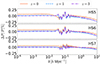 |
Fig. 1. Relative difference between EFTCAMB and MGCAMB for the linear matter power spectrum (ΔP/P ≡ [PEFTCAMB − PMGCAMB]/PMGCAMB) at three different redshifts, z = 0 (solid orange line), z = 1 (dashed blue line), and z = 3 (dot-dashed purple line) for the three fiducial models with |fR0| = 5 × 10⁻⁵ (HS5), |fR0| = 5 × 10⁻⁶ (HS6), and |fR0| = 5 × 10⁻⁷ (HS7). |
Finally, the scale-dependent μ function in Eq. (10) introduces a scale-dependent growth of structures, as shown by Zhang (2006) and Song et al. (2007). In Fig. 2, we plot the growth rate of perturbations, f(k, a)≡dlnδ/dlna, in f(R) Hu–Sawicki gravity with respect to that in ΛCDM, for three different scales k, namely 5 × 10⁻³ (solid blue line), 5 × 10⁻² (dashed purple line) and 5 × 10⁻¹h Mpc−1 (dot-dashed orange line), as a function of redshift from z = 0 to 2.5. This shows that the growth of perturbations at large scales is very similar to the one in standard GR at the redshifts of interest for large-scale structure formation. However, at smaller scales (larger k) the growth of perturbations is enhanced in f(R) at low redshifts (see Bueno Belloso et al. 2011, for a parametrisation of the growth rate in generic f(R) models, in terms of the growth index γ). These very features also complicate observational modelling, which in addition serves as a stress test of the forecast pipeline for constraints on theories beyond ΛCDM.
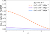 |
Fig. 2. Ratio of the scale-dependent matter growth rate f(k, z) in f(R) gravity (for the fiducial value |fR0| = 5 × 10⁻⁶) with respect to ΛCDM for three different wavenumbers, 5 × 10⁻³ (solid blue line), 5 × 10⁻² (dashed purple line), and 5 × 10⁻¹ h Mpc−1 (dot-dashed orange line), as a function of redshift from z = 0 to z = 2.5. The smaller the spatial scales and the lower the redshifts, the larger the enhancement of the growth rate compared to ΛCDM. |
3. Theoretical predictions for Euclid observables
As we describe in the next section, the forecasting methods and tools used in this paper are the same as those of EC20. However, we must note here that the change in the gravity theory introduced through the Hu–Sawicki model implies significant modifications of the recipes used to compute theoretical predictions for the Euclid observables. We discuss in this section how moving away from the standard GR assumption impacts the predictions for the angular power spectra, C(ℓ), that will be compared with the photometric survey data as well as the power spectra, Pobs, compared with data of the spectroscopic survey.
3.1. Photometric survey
For the Euclid photometric survey, the observables that need to be computed and compared with the data are the angular power spectra for WL, GCph, and their cross-correlation, XCph. In EC20 these were calculated using the Limber approximation plus the flat-sky approximation with the prefactor set to unity in a flat ΛCDM Universe:
 (13)
(13)
Here, kℓ = (ℓ+1/2)/r(z), r(z) is the comoving distance to redshift z = 1/a − 1, and Pδδ(kℓ, z) is the non-linear power spectrum of matter density fluctuations, δ, at wave number kℓ and redshift z in the redshift range of the integral from zmin = 0.001 to zmax = 4. The dimensionless Hubble function is defined as E(z) = H(z)/H0, and in all subsequent equations, H0 is expressed in units of km s−1 Mpc−1.
For each tomographic redshift bin i, the window functions WiX(z) with X = {L, G} (corresponding to WL and GCph, respectively) need to be computed differently with respect to what was done in EC20 as, when abandoning the assumption of a GR gravity theory, one has to account for changes in the evolution of both the homogeneous background and of cosmological perturbations. However, in the case of the f(R) model considered in this work, the background is ΛCDM up to a high precision. In general, one also has to account for both the modified evolution of the Bardeen potentials, Φ and Ψ, and the fact that in MG, the GR relation Φ = Ψ is not necessarily satisfied. Using the modified Poisson equation for Φ + Ψ of Eq. (7), this combination can be related to Pδδ as
![Mathematical equation: $$ \begin{aligned} P_{\Phi +\Psi }(k,z) = \left[-3{\Omega _{\mathrm{m} ,0}} \left(\frac{H_0}{c}\right)^2(1+z)\Sigma (k,z)\right]^2P_{\delta \delta }(k,z)\,, \end{aligned} $$](/articles/aa/full_html/2026/03/aa48713-23/aa48713-23-eq21.gif) (14)
(14)
where we assumed a standard background evolution of the matter component, i.e. ρm(z) = ρm, 0(1 + z)3, and Pδδ is computed accounting for the MG effects introduced through Eq. (5).
We can therefore use the recipe of Eq. (13) accounting for the effects of these modifications of gravity, not general modifications, for example, if matter coupling shifts Ωm(a). We can calculate H, r, and Pδδ, provided by dedicated Boltzmann solvers, but with the new window functions (Spurio Mancini et al. 2019)
 (15)
(15)
 (16)
(16)
where  and bi(k, z) are, respectively, the normalised galaxy distribution and the galaxy bias in the i-th redshift bin, and WiIA(k, z) encodes the contribution of intrinsic alignments (IAs) to the WL power spectrum. We followed EC20 in assuming an effective scale-independent galaxy bias. The main reason for this choice is to be able to compare it with the standard analysis with the modified gravity model as the only variable. Accounting for a scale-dependent galaxy bias would introduce further degrees of freedom that could confuse the comparison between the different cosmological models. A detailed analysis of both the concordance model and modified gravity theories that account for scale-dependent galaxy bias is beyond the scope of this work (see e.g. Tutusaus et al. 2020, for an analysis on the concordance model with a local, non-linear galaxy bias model).
The IA contribution is computed following the eNLA model from EC20, in which
 (17)
(17)
where
![Mathematical equation: $$ \begin{aligned} \mathcal{F} _{\rm IA}(z) = (1+z)^{\eta _{\rm IA}}\left[\frac{\langle L\rangle (z)}{L_\star (z)}\right]^{\beta _{\rm IA}}\,, \end{aligned} $$](/articles/aa/full_html/2026/03/aa48713-23/aa48713-23-eq26.gif) (18)
(18)
with ⟨L⟩(z) and L★(z) redshift-dependent mean and the characteristic luminosity of source galaxies as computed from the luminosity function, 𝒜IA, βIA, and ηIA are the nuisance parameters of the model, and 𝒞IA is a constant accounting for dimensional units. See Appendix for their respective meanings and values.
Changes in the theory of gravity impact the IA contribution introducing a scale dependence through the modified perturbations growth. This is explicitly taken into account in Eq. (17) through the matter perturbation δ(k, z), which is considered to be scale dependent in this case. This also allowed us to consider the scale dependence introduced by massive neutrinos, which was assumed to be negligible in EC20.
We note that while the window function for WL includes the MG function Σ to properly account for the modifications to Φ + Ψ, the GCph one does not have any explicit MG contribution, as the modifications to the clustering of matter are taken into account in the new Pδδ(kℓ, z).
We can therefore apply this recipe to the Hu–Sawicki f(R) model. Given our choice of the fiducial fR0, discussed in Sect. 4, the background modifications with respect to ΛCDM are negligible, while this model affects the evolution of perturbations, and therefore Pδδ, through Eq. (5), with the μ function given by Eq. (10).
The function Σ needs to relate the Φ + Ψ and matter power spectra, as in Eq. (14), and it is given by Eq. (12). As previously discussed for our fiducial choice, |fR0|≪1, the deviations of Σ from unity are negligible, and therefore the geometrical part of the lensing kernel entering Eq. (16) reduces to the standard one.
3.2. Spectroscopic survey
To exploit the data from the Euclid spectroscopic survey, we needed to compute the theoretical prediction for the observed galaxy power spectrum in the extended model considered here. The full non-linear model for the observed galaxy power spectrum is given by
![Mathematical equation: $$ \begin{aligned} P_\text{obs}(k_\text{ref},\mu _{\theta ,\text{ ref}};z)&= \frac{1}{q_\perp ^2(z) q_\parallel (z)} \left\{ \frac{\left[b\sigma _8(k,z)+f\sigma _8(k,z)\mu _{\theta }^2\right]^2}{1+k^2\mu _{\theta }^2\sigma _{\rm p}^2(z)}\right\} \nonumber \\&\qquad \times \frac{P_\text{dw}(k,\mu _{\theta };z)}{\sigma _8^2(z)} F_z(k,\mu _{\theta };z) + P_\text{s}(z) \, , \end{aligned} $$](/articles/aa/full_html/2026/03/aa48713-23/aa48713-23-eq27.gif) (19)
(19)
where the Pdw(k, μ; z) is the de-wiggled power spectrum that models the smearing of the BAO features due to the displacement field of wavelengths smaller than the BAO scale,
 (20)
(20)
where the Pnw(k; z) is a ‘no-wiggle’ power spectrum with the same broad band shape as Pδδ(k; z) but without BAO features (see below for details on how we computed it).
In Eq. (19), k is the modulus of the wave vector k and μθ is the cosine of the angle θ between this vector and the line-of-sight direction  . These quantities on the right-hand side are functions of their counterparts at a reference cosmology, i.e. k ≡ k(kref), μθ ≡ μθ, ref, which are transformed due to the Alcock-Paczynski effect; see EC20 and Casas et al. (2024) for the explicit formula. This transform, which also scales the overall Pobs is parameterised in terms of the angular diameter distance DA(z) and the Hubble parameter H(z) as
 (21)
(21)
 (22)
(22)
The term in the curly brackets in Eq. (19) is the contribution of redshift space distortions (RSD) corrected for the non-linear Finger-of-God (FoG) effect, where we defined bσ8(k, z) as the product of the effective scale-dependent bias of galaxy samples and the rms matter density fluctuation σ8(z); similarly, fσ8(k, z) is the product of the scale-dependent growth rate and σ8(z). As in the photometric survey, we follow EC20 in using an effective scale-independent galaxy bias. An analysis of modified gravity with scale-dependent galaxy bias models is left for future work.
The observed galaxy power spectrum is modulated by the redshift uncertainties, which manifest as a smearing of the galaxy density field along the line of sight. Hence, the factor Fz in Eq. (19) reads as
 (23)
(23)
Here, σr2(z) = c(1 + z)σ0, z/H(z) and σ0, z is the error on the measured redshifts.
Finally, Ps(z) is a scale-independent shot noise term, which enters as a nuisance parameter (see EC20).
The change in the gravity model affects the way to compute the theoretical predictions, as these expressions need to account for the possibility that the growth rate f(z) also depends on the wave number k. In general, this is the case for any MG model and also when perturbations in the dark energy sector are considered. For the model considered in this article, the only terms affected are those directly related to the growth rate, namely, f(k, z) itself and the two phenomenological parameters related to the velocity dispersion, σv, and the pairwise velocity dispersion, σp. These are
![Mathematical equation: $$ \begin{aligned} \sigma ^2_{\rm v}(z, \mu _{\theta })&= \frac{1}{6\pi ^2}\int \mathrm{d} k\, P_{\delta \delta }(k,z)\left\{ 1 - \mu _{\theta }^2 + \mu _{\theta }^2\left[1+f(k,z)\right]^2\right\} ,\end{aligned} $$](/articles/aa/full_html/2026/03/aa48713-23/aa48713-23-eq33.gif) (24)
(24)
 (25)
(25)
The phenomenological parameters σv(z, μθ) and σp(z) explain the damping of the BAO features and the FoG effect, respectively. The smearing of the BAO peak is due to the bulk motion of scales smaller than the BAO scale. For the power spectrum, this can be modeled in the Zeldovich approximation by a multiplicative damping term of the form exp[−kikj⟨di(z)dj(z)⟩], where ⟨di(z)dj(z)⟩ is the correlation function of the displacement field di evaluated at zero distance (see for instance the Appendix C of Peloso et al. 2015 for more details). Finally, we would like to clarify that in Eq. (20) we used the function gμ to express the damping of the BAO features in the matter power spectrum to keep the recipe closer to EC20; in this work, gμ = σv(z, μθ).
In ΛCDM model the growth rate is scale independent and both Eqs. (24) and (25) are the same (see EC20). We note that even if these parameters are assumed to be the same, they come from two different physical effects, namely large-scale bulk flow for the former and virial motion for the latter. Finally, due to the scale dependence of σp and σv, we evaluated both parameters in each redshift bin, but kept them fixed in the Fisher matrix analysis. This method corresponds to the optimistic settings in EC20. We would like to highlight that in this work we take directly the derivatives of the observed galaxy power spectrum with respect to the final parameters. This is in contrast to EC20 where we first performed the Fisher matrix analysis for the redshift-dependent parameters H(z), DA(z) and fσ8(z), and then projected to the final cosmological parameters of interest. Using the Euclid spectroscopic probe to measure the scale-dependence of the growth rate of structure formation, above the expected effect of neutrinos, would be a smoking gun for modified gravity. However, the forecasting method we apply here, using direct derivatives of the observed galaxy power spectrum, does not allow us to do this easily in the Fisher approximation. Neither was the case in EC20 with the “projection” method. For this, we would need a binning in k-modes, calculate Fisher matrices for each of these larger k-bins and have a good estimation of the covariance among those bins. This has been attempted previously in (Hojjati et al. 2012), but we we leave this for future work.
The no-wiggle matter power spectrum Pnw(k; z) entering Eq. (20) has been obtained using a Savitzky–Golay filter in the matter power spectrum Pδδ(k; z). The Savitzky–Golay filter is usually applied to noisy data to smooth their behaviour. This convolution method consists of fitting successive subsets of adjacent data points with a low-order polynomial. If the data are equally spaced (as is in our case, equally spaced in log10 k), then an analytic solution to the least-squares can be found as a series of coefficients that can be applied to all the subsets. In practice, using the Savitzky–Golay filter, we recover exactly the same shape and amplitude of the matter power spectrum without the BAO wiggles. While in EC20 we used the Eisenstein–Hu fitting formula (Eisenstein & Hu 1998) for the no-wiggle power spectrum, this is a fitting formula that only applies approximately to ΛCDM models and therefore cannot be straightforwardly applied in our case. We find that the Savitzky–Golay (SG) method is more accurate for models where the growth of matter density field depends on the scale k. The aforementioned smoothing filter has also been used in previous works (Boyle & Komatsu 2018) to reconstruct the neutrinos masses from galaxy redshift survey. In Fig. A.1 we plot our reconstruction of the wiggles computed with the Eisenstein–Hu formula compared to the SG method used in this work, where we can see that it performs very well also in the case of f(R).
3.3. Non-linear modelling for the spectroscopic probe
In the present analysis, for the spectroscopic probe, we adopt the non-linear modeling described above in Eq. (19) as it represents a minimal modification to what was used in the ΛCDM forecasts of EC20. This is a full-shape analysis with phenomenological terms that account for the quasi-linear evolution of biased tracers in redshift space. In our baseline analysis, we leave the σp and σv parameters fixed and also assume a scale-independent galaxy bias, which is a good approximation for very large scales. For our baseline settings, we chose to follow this more simplistic route, and it allowed us to have a clean comparison with EC20 with fixed theoretical systematics. However, it is worth noting that the state-of-the-art, based e.g. on the Taruya-Nishimichi-Saito model (Taruya et al. 2010) or on perturbation theory prescriptions based on the Effective Field Theory of Large Scale Structure (EFToLSS, see Carrasco et al. 2012, and references therein), has been implemented in the analysis of real data from the BOSS survey (Song et al. 2015; Colas et al. 2020) and the DESI2 survey (DESI Collaboration 2025); NovellMasot:2025fju. Furthermore, eBOSS analyses (Beutler et al. 2014, 2017; de Mattia et al. 2021), as well as forecasts for unbiased parameter estimation for Stage IV cosmological surveys, show that the choice of kmax is not universal (see e.g. Markovic et al. 2019), and different kmax for the monopole, quadrupole, and hexadecapole are required (the kmax for the latter is considerably smaller). Therefore, we study several kmax choices for the full shape of the power spectrum of spectroscopically observed galaxies. In Linde et al. (2024) the authors have tested these EFToLSS predictions against our phenomenological model described here and have found that for intermediate scales, the error bars are of similar magnitude when opening the parameters σp and σv in each redshift bin. In this case, the number of nuisance parameters increases to 8 for our 4 redshift bins. In this case, the fiducial values of these velocity dispersion parameters are calculated using Eqs. (24) and (25) and they are varied in the Fisher analysis with a rescaling parameter, the fiducial value of which is unity. Regarding the galaxy bias, we use the so-called ‘Q-bias’ approximation (see Song et al. 2015) with the scale-dependent form
 (26)
(26)
and we took the fiducial values for these two parameters A1[h−1 Mpc] and A2 [h−2 Mpc2] based on previous work done in Euclid Collaboration: Bose et al. (2024), where a χ2-analysis was performed on simulated data for the HS6 f(R) Hu–Sawicki model. The values of these nuisance parameters can be found in Table B.1.
In the presence of massive neutrinos, most of these formalisms would need further adjustments, as there is a degeneracy between the scale-dependent power spectrum damping induced by the free-streaming of neutrinos and the scale-dependent and growth-enhancing effect of the fifth force in f(R) (see Baldi et al. 2014). There is the possibility of breaking this degeneracy, by using information on redshift space distortions. This involves extending the perturbation theory modeling (Wright et al. 2019) or performing a detailed comparison with galaxy mocks from simulations (García-Farieta et al. 2019). However, in Bose et al. (2020) it has been shown that at the scales probed by Euclid and with realistic error bars and taking into account the necessary screening mechanisms, the f(R) modelling can be well approximated by leaving the perturbation theory kernels intact.
3.4. Non-linear modelling for the photometric probe
While for the galaxy power spectrum on mildly non-linear scales we use a modified version of the model in EC20, we do not have, in general, an analytical solution for the deeply non-linear power spectrum in a f(R) cosmology. In this work, we therefore use a fitting formula designed in Winther et al. (2019) that captures the enhancement in the power spectrum compared to a ΛCDM non-linear power spectrum, as a function of the parameter fR0. This fitting function has been calibrated using the DUSTGRAIN (Giocoli et al. 2018) and the ELEPHANT (Cautun et al. 2018) N-body simulations (see Winther et al. 2015, for a comparison of different N-body codes for f(R) cosmologies).
The fitting function we used is given by
 (27)
(27)
where the {Xi} are themselves functions of fR0 and redshift, X ≡ X(z; fR0). The redshift dependence is a polynomial relation to the scale factor a = 1/(1 + z) given by
 (28)
(28)
with each Xij coefficient in itself defined as a polynomial in  given by
 (29)
(29)
With three indices for Xijk, this gives in total 6 × 3 × 3 = 54 free parameters for the scale, redshift and fR0 dependence. The response function, Ξ(k, z), is the ratio of the non-linear matter power spectrum in f(R) theory to the non-linear spectrum calculated within the ΛCDM model. The fitting formula Eq. (27) found in Winther et al. (2019) is a direct fit to the ratio Ξ(k, z). This fitting formula is not defined outside the range 10−4 < |fR0| < 10−7, and therefore this limits our smallest fiducial value for |fR0| across probes to 5 × 10⁻⁷ since we need to be far from the lower limit to be able to compute the numerical derivatives accurately. In Fig. 3 we plot the function Ξ(k, z) for each of the fiducial |fR0| values chosen in this model, namely 5 × 10⁻⁵ (blue line), 5 × 10⁻⁶ (purple line), and 5 × 10⁻⁷ (orange line), as a function of scale k. To compare the enhancement with respect to ΛCDM in our redshifts of interest, we evaluate it at z = 0.25 (solid lines) and z = 1.75 (dashed lines). These redshifts correspond approximately to the means of the first and last lensing tomographic bins of our survey, respectively (see Sect. 4) also Fig. 3. As can already be seen from this figure, the enhancement with respect to ΛCDM decreases rapidly with a smaller |fR0| value; therefore, we expect to have worst constraints for smaller values of |fR0| when testing this model against probes that are sensitive to the deeply non-linear power spectrum. We note, however, that the Fisher matrix sensitivity is dominated by the response of this function to small changes in |fR0| (i.e. its first derivatives), which can become large at small scales, and therefore we can obtain relatively tight constraints, even if the absolute enhancement compared to ΛCDM is of just a few percent when evaluated at the fiducial cosmology. In Sect. 4 we specify our choice of fiducial parameters for each model.
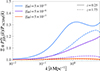 |
Fig. 3. Ratio of the non-linear power spectrum in f(R) gravity to ΛCDM from the fitting function in Eq. (27) for three different values of the |fR0| parameter, namely, 5 × 10⁻⁵ (blue line), 5 × 10⁻⁶ (purple line), and 5 × 10⁻⁷ (orange line), as a function of scale, k, evaluated at two different redshifts, z = 0.25 (solid lines) and z = 1.75 (dashed lines). These redshifts correspond approximately to the means of the first and last lensing tomographic bins of our survey, respectively (see Section 4). The fitting formula designed in Winther et al. (2019) is not defined outside 10−7 < |fR0| < 10−4. |
We implemented Ξ(k, z) into the Boltzmann codes MGCAMB and EFTCAMB, and to obtain the non-linear f(R) matter power spectrum, we then multiplied Ξ(k, z) by a ΛCDM non-linear spectrum,  . For the ΛCDM power spectrum PΛCDM(k, z), we use the Halofit ‘Takahashi’ prescription (Takahashi et al. 2012), as this is the prescription most readily available in MGCAMB, and also the prescription used in Winther et al. (2019) to test the fitting formula against N-body simulations. During the preparation of this work, an emulator for the deeply non-linear matter power spectrum has been developed by the Euclid collaboration, the EuclidEmulator (see Euclid Collaboration: Knabenhans et al. 2019, for details on its implementation), calibrated on the Euclid Flagship simulation (Potter et al. 2017). Whilst it might be interesting to use it in the future, the current available version, EuclidEmulator2 (see Euclid Collaboration: Knabenhans et al. 2021), offers a Python wrapper to the Boltzmann code CLASS (Lesgourgues 2011); Blas:2011rf rather than to MGCAMB and EFTCAMB we use for this paper; we are therefore not using the EuclidEmulator in the current analysis (see Sect. 2). Also, during the preparation of this work, an emulator for the non-linear matter power spectrum in |fR0| was developed by Arnold et al. (2022) and goes under the acronym FORGE. The authors of this papers have independently checked that this emulator agrees well with the fitting formula by Winther et al. (2019) around the fiducial values of interest. However, this FORGE emulator has been calibrated with massless neutrino simulations and allows only for variations of the cosmological parameters Ωm, 0, σ8, and h. Since in this work we want to have the flexibility to vary all other cosmological parameters and also the ability to connect to accurate modified gravity Boltzmann codes, we leave the application of this emulator for future work. The fitting formula in Winther et al. (2019) is also checked to be valid in the presence of non-zero neutrino masses, using data from Baldi et al. (2014). With the value ∑mν = 0.06 eV chosen in this work, this fitting formula is accurate enough across our ranges of scales and redshifts of interest.
For the photometric observables, we are probing up to smaller scales. For this reason, including nuisance parameters about baryonic feedback on the matter power spectrum would be necessary for unbiased parameter estimation, and it would also possibly entail a degradation of the constraints from WL (see e.g. Schneider et al. 2020a,b). However, at the moment, we do not have accurate Euclid-like simulations that include baryonic effects, especially in the case of MG cosmologies. Therefore, we ignore these effects in our analysis, leaving them for future work.
We are aware that there are important degeneracies among the effect of f(R) and neutrino masses, especially at non-linear scales (see e.g. Hu et al. 2015; Baldi et al. 2014). Although massive neutrinos suppress the power spectrum at small scales, on the one hand, f(R) will increase clustering at a similar range of scales, therefore partially cancelling the former effect (Baldi et al. 2014). Ignoring these degeneracies might artificially tighten our constraints on |fR0| since we would be considering a much higher signal than the one actually present under a large sum of neutrino masses (He 2013; Motohashi et al. 2013; Harnois-Déraps et al. 2015). Breaking these degeneracies is possible, either by using statistics on the cosmic web (Shim et al. 2014), higher than second-order statistics in weak lensing (Peel et al. 2018; Giocoli et al. 2018), or machine learning (Peel et al. 2019; Merten et al. 2019). However, these techniques are beyond the scope of this work. Galaxy clusters and voids also offer the possibility of distinguishing between these two possible scenarios, as investigated in Hagstotz et al. (2019a, b), Ryu et al. (2020), and Contarini et al. (2021).
4. Survey specifications and analysis method
In order to forecast constraints on this specific model, we follow the same approach as EC20. We adopt the same Fisher matrix formalism, as well as the codes validated therein. Given that the theoretical model considered is crucially different, we update the forecast recipe and the corresponding codes as described in the previous section. The cosmological parameters here considered and their fiducial values, for which we again followed EC20, read
 (30)
(30)
The fiducial values of σ8 shown above are obtained keeping the scalar amplitude of the primordial power spectrum As fixed for the three cosmologies. Given the impact of the f(R) model under examination, this leads to σ8 values that appear in tension with currently available results. However, it is important to stress that the comparison should be done with modified gravity analyses of the present data, rather than with results obtained assuming ΛCDM. In fact, the fiducial values of σ8 we quote are compatible with such analyses, as degeneracies between σ8 and modified gravity parameters increase the mean value of the former while also broadening the constraints (see e.g. Abbott et al. 2023).
In the following text and in the figures, we refer to the model with the corresponding |fR0| = 5 × 10⁻⁵ fiducial as HS5, the model with |fR0| = 5 × 10⁻⁶ as HS6 and the model with a fiducial value of |fR0| = 5 × 10⁻⁷ as HS7. The baseline fiducial used for the rest of this work is the HS6 model since it corresponds to a value of |fR0| still allowed by observations and with enough distinctive signatures with respect to ΛCDM to be detected by future observations. We note that our fiducial cosmology includes massive neutrinos with a total mass of ∑mν = 0.06 eV, but we keep ∑mν fixed in the following Fisher matrix analysis. We also use the same initial amplitude of primordial perturbations for both fiducial models, namely As = 2.12605 × 10⁻⁹. As discussed previously in Sect. 3.4, fixing neutrino masses ignores the degeneracies between their effect on the power spectrum and the increase of clustering at small scales; therefore, our constraints might be tighter than in a scenario in which also ∑mν is varied.
Concerning the photometric probes, the galaxy distribution was binned into ten equally populated redshift bins with an overall distribution following
![Mathematical equation: $$ \begin{aligned} n(z)\propto \left(\frac{z}{z_0}\right)^2\,\text{ exp}\left[-\left(\frac{z}{z_0}\right)^{3/2}\right], \end{aligned} $$](/articles/aa/full_html/2026/03/aa48713-23/aa48713-23-eq42.gif) (31)
(31)
with  and the normalisation set by the requirement that the surface density of galaxies is
  . The redshift distribution was then convolved with a sum of two Gaussian distributions to account for the photometric redshift uncertainties (see EC20, for details). The galaxy bias was assumed to be constant within each redshift bin. Its values, bi, were introduced as nuisance parameters in our analysis, with their fiducial values determined by
  , where
  is the mean redshift of each redshift bin. Even though deviations from GR introduce, in principle, a scale dependence also in the galaxy bias, we assumed that this is negligible in our case.
Moreover, we followed EC20 in accounting for a Gaussian covariance between the different photometric probes:
![Mathematical equation: $$ \begin{aligned}&\text{ Cov}\left[C_{ij}^{AB}(\ell ),C_{kl}^{CD}(\ell ^{\prime })\right]=\frac{\delta _{\ell \ell ^{\prime }}^\mathrm{K}}{(2\ell +1)f_{\rm sky}\Delta \ell }\nonumber \\&\quad \times \left\{ \left[C_{ik}^{AC}(\ell )+N_{ik}^{AC}(\ell )\right]\left[C_{jl}^{BD}(\ell ^{\prime })+N_{jl}^{BD}(\ell ^{\prime })\right]\right.\nonumber \\&\qquad \qquad +\left.\left[C_{il}^{AD}(\ell )+N_{il}^{AD}(\ell )\right]\left[C_{jk}^{BC}(\ell ^{\prime })+N_{jk}^{BC}(\ell ^{\prime })\right]\right\} \,, \end{aligned} $$](/articles/aa/full_html/2026/03/aa48713-23/aa48713-23-eq47.gif) (32)
(32)
where upper-case Latin indexes A, … = {WL, GCph}; lower-case Latin indexes i, … run over all tomographic bins; δℓℓ′K is the Kronecker delta symbol; fsky ≃ 0.36 represents the fraction of the sky observed by Euclid; and Δℓ denotes the width of the multipole bins, where we used 100 equally spaced bins in log-space. The noise terms, which for the observables considered here are in fact white noise, namely  , read
 (33)
(33)
 (34)
(34)
 (35)
(35)
where σϵ2 = 0.32 is the variance of observed ellipticites.
For the spectroscopic probe, we evaluated the Fisher matrix Fαβ(zi) for the observed galaxy power spectrum according to the recipe outlined in EC20 (see Sect. 3.2). Here, α and β run over the cosmological parameters of the set Θ, the index i labels the redshift bin, each respectively centred in zi = {1.0, 1.2, 1.4, 1.65}, whose widths are Δz = 0.2 for the first three bins and Δz = 0.3 for the last bin. In this paper, in comparison to EC20, we adopt the direct derivative approach, i.e. we vary the observed galaxy power spectrum with respect to the cosmological parameters of Θ directly, plus two additional redshift-dependent parameters lnbσ8(zi) and Ps(zi) that we marginalise over. We consider the numerical values for the galaxy bias, b(z), and the expected number density of the observed Hα emitters, n(z), reported in Table 3 of EC203.
For both probes, we consider two different settings: an optimistic and a pessimistic case. In the optimistic case, we consider kmax = 0.30 h Mpc−1 for GCsp, ℓmax = 5000 for WL, and ℓmax = 3000 for GCph and XCph. Instead, in a pessimistic setting, we consider kmax = 0.25 h Mpc−1 for GCsp, ℓmax = 1500 for WL, and ℓmax = 750 for GCph and XCph. Based on recent work on updated Markov chain Monte Carlo forecasts by the Euclid collaboration Euclid Collaboration: Mellier et al. (2025) and Euclid Collaboration: Archidiacono et al. (2025; specifically for the neutrino sector), we adopted the pessimistic scenario as our baseline setting, as we believe this represents a more conservative estimation of the constraining power of the mission given the yet unknown systematics modelling.
At the smallest photometric redshift bin, the galaxy number density distribution n(z) peaks around z = 0.25, which means that under the Limber approximation and for our fiducial cosmology, the corresponding maximum values of k evaluated in the power spectrum corresponding to the pessimistic and optimistic settings for GCph are kmax = [0.7, 2.9] h Mpc−1, respectively, and for WL the maximum wave-numbers probed are kmax = [1.4, 4.8] h Mpc−1 for pessimistic and optimistic, respectively. For smaller values of z, the values of k at a given ℓ increase monotonically, but there the window functions in Eq. (15) and Eq. (16) suppress the power spectrum, and we set it to zero after a fixed kmax = 30 h Mpc−1. In both settings, we fix the nuiscance parameters σp and σv for GCsp, which we calculate directly from Eqs. (24) and (25) for the fiducial value of the cosmological parameters. In Appendix we show the results for a more conservative setting, in which σp and σv are varied freely at each redshift bin and we marginalise as well over two parameters for the scale-dependent galaxy bias; see Eq. (26). In practice, the real constraining power will lie between these two extremes, as the future improvements in modelling and the priors obtained from simulations enable us to pin down the large number of free nuisance parameters. We also performed a pessimistic quasi-linear forecast for GCsp only, where we set our maximum wave number at kmax = 0.15 h Mpc−1 in order to have a more conservative estimate of the constraining power of the GCsp probe. The reason for this is that the underlying matter power spectrum of Eq. (19) that we are using in our observed galaxy power spectrum recipe is a linear one, as we detailed in Sect. 3.2. It is known that non-linear corrections start playing a role above scales of around k = 0.1 h Mpc−1 for the redshifts under consideration (see Taruya et al. 2010) and, therefore, the use of a linear power spectrum beyond these scales can bias our constraints. Hence, we aim to estimate what would happen if we used just quasi-linear scales in the analysis. As shown in Sect. 5, the effect of these two different scale cuts on the constraining power on the log10|fR0| parameter is minimal for our GCsp recipe. As a reference for the reader, we list the specific scale choices and settings used for each observable in Table 1.
Euclid survey specifications for WL, GCph, and GCsp.
In this work, as in EC20, we show the results for most of these single probes, but also for their combinations. It is important to mention that when we consider the combination of GCph with WL, we neglect any cross-correlation. However, when we add their cross-correlation XCph, we include them both in the data vector and in the covariance, i.e. we perform a full analysis taking into account the cross-covariances between GCph, WL, and their cross-correlation. This combination of three distinct two-point correlation functions is also known in the literature as 3 × 2 pt, and we use this terminology interchangeably in this work. Moreover, again following EC20, we do not present the values for GCph alone. The main reason for this choice is that we consider both σ8 and the galaxy biases as parameters, which are degenerate in the linear regime. Even if this degeneracy might be partially broken when adding non-linear information, the Fisher formalism can still manifest numerical instabilities for this single probe alone. Therefore, we always show the constraints from GCph in combination with other probes. In the optimistic setting, we assume that GCsp is uncorrelated with photometric probes. In the pessimistic setting, we neglect any correlation between GCsp and WL, and also apply a redshift cut at z < 0.9 for GCph and XCph, in order to minimise the overlap between the different galaxy clustering probes. However, we note that this redshift cut is only applied when combining spectroscopic and photometric data. Even in the pessimistic case, we do not apply any redshift cut when considering photometric data alone.
Finally, in this work, we have validated again the codes used in EC20 to account for the modified recipe outlined in the previous sections. We have compared, for the constraint on each parameter of Θ and the nuisance parameters of each probe, the performance of each independent code with the median of the constraints obtained by the available codes. We have verified that the relative difference in percentage between a given code and such a median is always below 10%, both for marginalised and unmarginalised parameters, which was the threshold for code consistency adopted in EC20 and more recently in Casas et al. (2024). Concerning the spectroscopic probes, here we have corrected for an inconsistency in the unit conversion from Mpc−1 to h Mpc−1 units that affected previous forecasts; thus, the sensitivity to h degrades with respect to EC20, while the sensitivity to the other cosmological parameters is only mildly altered due to their small correlations with h. This mistake was also present in Casas et al. (2024) and we have checked that manually reintroducing this bug yields the same constraints for ΛCDM as reported there. The pipeline used for this paper is the publicly available4CosmicFishPie code, which has been validated in Casas et al. (2024) against Markov chain Monte Carlo pipelines and is inspired by the original code used in EC20. After publication, the notebooks for reproducing the figures in this paper will be available in an example directory of Cosmicfispie .
.
5. Results
5.1. Pessimistic baseline setting
As shown in Eq. (30), we have chosen three different fiducial values of the Hu–Sawicki f(R) model parameter, namely |fR0| = 5 × 10⁻⁷ (HS7), |fR0| = 5 × 10⁻⁶ (HS6) and |fR0| = 5 × 10⁻⁵ (HS5), based on our discussion of current observational constraints in Sect. 1. We employ HS7, which contains a very small value of |fR0| as our GR-limit test, since we cannot correctly perform forecasts at lower values of |fR0| due to the limitations we have in the non-linear modelling with the Winther fitting formula mentioned in Sect. 3.4. We remind the reader of the two considered settings, pessimistic and optimistic, as explained in Sect. 4 plus the ‘quasi-linear’ setting for GCsp, defined by kmax = 0.15 h Mpc−1.
For our baseline fiducial (HS6) and our baseline settings, Euclid alone will be able to constrain the additional parameter log10|fR0|, which has a value of log10|fR0| = −5.301 at the 1σ level with an absolute error of
-
σlog10|fR0| = 0.20 with spectroscopic GCsp alone
(corresponding to a relative 3.9% error);
-
σlog10|fR0| = 0.43 with WL alone
(corresponding to a relative 8.3% error);
-
σlog10|fR0| = 0.14 combining WL, GCph, and XCph
(corresponding to a relative 2.7% error);
-
σlog10|fR0| = 0.95 using the full combination GCsp + WL +
GCph + XCph (corresponding to a relative 1.8% error).
In Table 2 and in Fig. 4, we list the forecasted 1σ fully marginalised errors (relative errors to its fiducial) on all the cosmological parameters considered for our model with |fR0| = 5 × 10⁻⁶ (HS6), for the individual probes and their combinations in the pessimistic setting. The probes shown are GCsp (in purple), WL (in blue), GCsp + WL (orange), the 3 × 2 pt combination of all photometric probes, including cross correlations, WL + GCph + XCph (red) and the combination of all spectroscopic and photometric probes GCsp + WL + GCph + XCph (yellow). We keep the same color convention in all figures of the article when showing constraints from different probes. Table 2 contains this information also for the pessimistic survey settings.
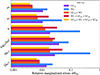 |
Fig. 4. Marginalised 1σ errors on cosmological parameters relative to their corresponding fiducial value for the pessimistic baseline case, which equals to |fR0| = 5 × 10⁻⁶. We show results for GCsp (purple); WL (blue); GCsp + WL (orange); the combination of all photometric probes, including cross correlations, WL + GCph + XCph (red); and the combination of all spectroscopic and photometric probes, GCsp + WL + GCph + XCph, (yellow). One can see that the constraints on log10|fR0| and σ8 are similar among GCsp and WL, but for other parameters such as the Hubble parameter, h, or the fraction of baryons, Ωb, 0, the constraints coming from GCsp alone are even more stringent than the constraints of all photometric probes combined on their own. |
Forecast 1σ marginal relative errors on the cosmological parameters for a flat f(R) model with |fR0| = 5 × 10⁻⁶ (log10|fR0| = −5.301) in the pessimistic and optimistic cases using Euclid observations of spectroscopic galaxy clustering (GCsp), WL, photometric galaxy clustering (GCph), and the cross-correlation among the photometric probes XCph.
In Fig. 5, we plot the elliptical 1σ and 2σ contours for the probes GCsp, WL, the combination GCsp + WL, and all the Euclid probes combined GCsp + WL + GCph + XCph, using the same colour convention mentioned before. From the parameters used in the Fisher matrix, we leave out this plot Ωb, 0 as it does not provide any additional information. As can be seen in this figure, GCsp is always better at constraining h and ns, compared to the cosmic shear probe (WL) alone. However, due to the orthogonality of the contours, especially in the subspaces that combine σ8 with ns and h, there is an important lifting of degeneracies, which makes the combination of GCsp and WL (shown in orange) much more constraining. The relative constraint on log10|fR0| coming from WL alone (blue) is of the order of 8%, this reduces by a factor 4 when combined with the spectroscopic probe (orange), with an extra 30% improvement in constraining power when adding all Euclid probes together (yellow), yielding in total a relative constraint on log10|fR0| of 1.8% in this pessimistic baseline setting. Throughout this work, we indicate the 1σ constraints rounded to the nearest significant digit, since our Fisher matrix method has been validated at the 10% level on the discrepancy between 1σ marginalised and unmarginalised errors on the cosmological and nuisance parameters, as mentioned in Sect. 4. In Appendix we explicitly show the contribution to the constraining power and the breaking of degeneracies from the GCsp probe itself. For the same HS6 model considered above, it can be seen in Fig. A.2 that it is the spectroscopic probe that helps break degeneracies in the h and Ωb, 0 planes, mainly due to the sensitivity of the BAO wiggles on these two parameters. The cosmic shear probe (WL) is relatively insensitive to Ωb, 0 and h and the full combination of photometric probes is also not good at constraining h. It is the breaking of degeneracies when combining GCsp and WL probes, that improves considerably the constraints on all parameters, showcasing the particular power of combining Euclid’s primary probes to measure parameters in and beyond the standard model of cosmology.
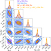 |
Fig. 5. Joint marginal error contours at 1σ and 2σ on the cosmological parameters for a flat f(R) model with |fR0| = 5 × 10⁻⁶ in the optimistic setting. Purple is for GCsp, blue for WL, orange for the combination GCsp + WL, and yellow for all the photometric probes including their cross-correlation XCph, combined with GCsp, namely GCsp + WL + GCph + XCph. While the WL probe is unable to properly constrain the Hubble parameter h and the primordial slope ns on its own, the orthogonality of the contours for GCsp and WL in the subspaces involving h and ns, helps lift degeneracies and further improves the fully marginalised constraints on log10|fR0|, when probe combinations are used. |
5.2. Constraints on the fundamental model parameter |fR0|
We note that we performed the Fisher matrix analysis on the parameter log10|fR0|, instead of directly on |fR0|, since for very small numbers and for large order of magnitude differences, the Fisher matrix derivatives might become unstable (see, e.g., Camera et al. 2018, Appendix A1). Therefore, it is recommended to have all the involved parameters in the Fisher matrix to be of the same order of magnitude. Since the transformation between log10|fR0| and |fR0| is non-linear and the parameter constraints are not small in some cases, we cannot simply use a Jacobian transformation to convert between the Fisher matrices in this case. Our assumption of Gaussianity is only true for the logarithmic parametrisation log10|fR0|. Therefore, the posterior contours for |fR0| will be non-Gaussian.
We can, nevertheless, obtain the fully marginalised constraints on |fR0| by transforming the log10|fR0| symmetric bounds
 (36)
(36)
into the upper and lower bounds for the linearly parameterised parameter |fR0|
 (37)
(37)
This will result in asymmetric errors in |fR0| since the upper and lower bounds will be given by the exponentiation of the symmetric 1σ bounds.
Using these formulas, we can obtain the upper and lower 1σ-bounds for our fiducial parameter |fR0| for the different cases
-
 with spectroscopic GCsp alone;
 -
 with WL alone;
 -
 combining WL, GCph, and XCph
 -
 with GCsp+WL+GCph+XCph.
As one can clearly see from these numbers, the stronger the constraint on the log10|fR0| parameter, the more symmetric the upper and lower bounds on |fR0| become, simply due to the central limit theorem and the fact that for a very peaked likelihood, a Gaussian approximation is always possible around the maximum of the posterior distribution.
In order to visualise this, we take our Fisher matrices computed for each of the cases and probes and assign them to a multivariate Gaussian distribution, by using the Fisher matrix as the inverse covariance. We then sample from this distribution and transform the samples of log10|fR0| into samples on |fR0| using the inverse of the logarithmic transformation, see Eq. (37). Using this technique, we plot on the left side of Fig. 6 the marginalised posterior 1D and 2D distributions for the original model parameter |fR0| in the HS6 case, for the optimistic setting, using the same colour convention as before. Compared to Fig. 5 we show now, for illustration purposes, the 3 × 2 pt combination of photometric probes (WL + GCph + XCph) in red, instead of the GCsp + WL combination, and we focus only on the parameters |fR0|, Ωm, 0 and σ8. We also remove the WL probe, since its constraints on |fR0| are weak. For the subspaces involving the |fR0| parameter, we now see non-symmetrical posterior distributions, which are clearly non-Gaussian, and noticing the marginalised 1D posterior distributions in the top of each sub-panel, we see that they have a longer tail on the upper side of the constraints. This asymmetry is also due to the fact that using the logarithmic parameterisation automatically prevents us from going into negative regions of the parameter space for |fR0|, and therefore the probability distributions are skewed towards the positive side. However, the stronger the constraints on this parameter (for example, in the case of the full combination of the Euclid probes, in yellow), the better the Gaussian approximation.
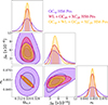 |
Fig. 6. Same as Fig. 5 (HS6) but for a subset of the cosmological parameters (omitting WL alone) when transforming the contours back into the fundamental parameter |fR0|. While in the logarithmic case the marginalised Fisher contours are simply Gaussians by definition, this is not the case for the contours on the linearly parameterised case |fR0|. For the probes GCsp (purple) and WL (blue) on their own which are less constraining, the errors on |fR0| are very asymmetric with heavy tails on the right. However, the smaller the 1σ marginalised error on log10|fR0| is, the better the marginalised posterior on |fR0| can be approximated by a Gaussian. This can be seen for the full combination of Euclid probes (yellow). |
5.3. Comparison of the HS5, HS6, and HS7 Hu–Sawicki models
In addition to our baseline fiducial for f(R) gravity, |fR0| = 5 × 10⁻⁶, we also perform forecasts on a second and third fiducial, namely |fR0| = 5 × 10⁻⁵ (HS5) and |fR0| = 5 × 10⁻⁷ (HS7), the latter is closer to ΛCDM in terms of perturbations and background evolution. A closer limit to ΛCDM is currently not possible using non-linear predictions, since our non-linear fitting formula discussed in Sect 3.4 cannot be extrapolated for values of the f(R) model parameter smaller than |fR0| = 5 × 10⁻⁷. We also perform forecasts on a flat ΛCDM model in order to have a comparison scenario within the assumptions of our recipe for the large scale structure probes.
In Table A.1 we report the 1σ fully marginalised forecasted errors for these models in the optimistic and pessimistic settings for the most important Euclid probe-combinations discussed above. For the HS5 model we find in general very similar constraints to HS6, but it is important to remark that due to the increased signal at non-linear scales and also the larger k-dependence of the growth, due to a higher value of |fR0|, we obtain better constraints on log10|fR0| for the full combination of probes, both in the pessimistic and optimistic settings, with relative errors of 1.3% and 0.6%, respectively. In the case of the HS7 model, the fiducial value of |fR0| is yet another order of magnitude closer to ΛCDM as compared to HS6, and therefore, we expected the extra signal on the power spectrum coming from modified gravity to be much smaller. We indeed find that this is the case, and compared to HS6, the relative percentage constraints on log10|fR0| degrade by a factor 3.6 in GCsp, a factor 4.9 in WL and a factor 3 when considering the full Euclid spectroscopic and photometric combination. The final relative constraint on log10|fR0| for this latter case is 1.8%, which corresponds to a determination of ![Mathematical equation: $ {|f_{R0}|}=[5.0^{+ 1.5}_{-1.1} \times 10^{-7}] $](/articles/aa/full_html/2026/03/aa48713-23/aa48713-23-eq60.gif) . In Fig. 7 we plot the confidence contours for this HS7 model in the baseline pessimistic setting compared to the HS6 baseline model. In dark purple/purple we plot the constraints for GCsp for HS7/HS6 and in dark red/red the constraints on the 3 × 2 pt photometric Euclid probe. For the standard cosmological parameters, such as in the subspace of Ωm, 0 vs. h or σ8, we can see that we recover very similar contours in size and in orientation. However, for the log10|fR0| parameter the ellipses in HS7 become considerably more elongated. For instance, one can see in the panel of log10|fR0| vs. σ8 that the GCsp probe alone is not sufficient to distinguish these two models from each other, but the full photometric combination is able to discriminate between them at more than 2σ. As discussed previously, this is under the assumption that both models have the same primordial amplitude and, therefore, due to a larger growth in the case of HS6, they end up with different values of σ8 today. To be certain that the choice of σ8 values does not affect our constraints, we performed a Fisher matrix forecast of the HS6 model, changing its primordial amplitude As, so that it has the same amplitude of fluctuations σ8 = 0.816 today as the baseline ΛCDM model. We found that none of the parameter constraints changed considerably with respect to the baseline HS6 case. We have also tested that when fixing the extra model parameter log10|fR0| in the HS7 model, which is the closest we have to ΛCDM and just deviates in the non-linear power spectrum and the growth rate function by a few percent (see Figs. 2 and 3), we then recover the same constraints on the five remaining ΛCDM parameters. This comparison is shown in the left panel of Fig. A.3, where in dark yellow we show the full combination of Euclid probes for the pessimistic HS7 case and in cyan the corresponding 1D and 2D contours for the ΛCDM scenario as described in EC20.
. In Fig. 7 we plot the confidence contours for this HS7 model in the baseline pessimistic setting compared to the HS6 baseline model. In dark purple/purple we plot the constraints for GCsp for HS7/HS6 and in dark red/red the constraints on the 3 × 2 pt photometric Euclid probe. For the standard cosmological parameters, such as in the subspace of Ωm, 0 vs. h or σ8, we can see that we recover very similar contours in size and in orientation. However, for the log10|fR0| parameter the ellipses in HS7 become considerably more elongated. For instance, one can see in the panel of log10|fR0| vs. σ8 that the GCsp probe alone is not sufficient to distinguish these two models from each other, but the full photometric combination is able to discriminate between them at more than 2σ. As discussed previously, this is under the assumption that both models have the same primordial amplitude and, therefore, due to a larger growth in the case of HS6, they end up with different values of σ8 today. To be certain that the choice of σ8 values does not affect our constraints, we performed a Fisher matrix forecast of the HS6 model, changing its primordial amplitude As, so that it has the same amplitude of fluctuations σ8 = 0.816 today as the baseline ΛCDM model. We found that none of the parameter constraints changed considerably with respect to the baseline HS6 case. We have also tested that when fixing the extra model parameter log10|fR0| in the HS7 model, which is the closest we have to ΛCDM and just deviates in the non-linear power spectrum and the growth rate function by a few percent (see Figs. 2 and 3), we then recover the same constraints on the five remaining ΛCDM parameters. This comparison is shown in the left panel of Fig. A.3, where in dark yellow we show the full combination of Euclid probes for the pessimistic HS7 case and in cyan the corresponding 1D and 2D contours for the ΛCDM scenario as described in EC20.
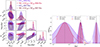 |
Fig. 7. Left: Joint marginal error contours at 1σ and 2σ on the cosmological parameters for a flat f(R) model with |fR0| = 5 × 10⁻⁶ (HS6) vs. |fR0| = 5 × 10⁻⁷ (HS7) in the pessimistic setting. Lighter colours and solid contours correspond to HS6, while darker colours and dashed empty contours correspond to HS7. In purple the spectroscopic GCsp, in red the combination of photometric probes (GCsp + WL + GCph + XCph). These two HS models only differ by their value of σ8 and log10|fR0|. Therefore the contours look very similar in the standard cosmological parameters. For log10|fR0| the ellipses become much more elongated in HS7. Right: One-dimensional fully marginalised posteriors on the |fR0| parameter for HS7 (dashed), HS6 (solid), and HS5 (dotted) after applying the transformation in Eq. (37). We use the same colour convention as before. The shaded vertical areas correspond to the 1σ confidence intervals, while the Gaussian curves extend up to 3σ. Using the full combination of photometric probes, HS7 and HS6 can be distinguished at 2σ, and both of them can be distinguished from HS5 at 3σ or more. |
On the right panel of Fig. 7, we compare now the constraints across the three models studied in this work, HS5 (in dotted lines), HS6 (in solid lines) and HS7 (in dashed lines) for the fundamental parameter |fR0|. We plot the 1D fully marginalised posterior on |fR0| for the spectroscopic probe GCsp on its own and the 3 × 2 pt photometric combination of probes, using again the same colour codes as before. The shaded areas under the curve represent the 1σ confidence intervals and the extent of the Gaussian curves corresponds to a 3σ deviation from the mean. Due to the logarithmic scale of the x-axis, the distributions look symmetric again, nevertheless, we can see that in absolute |fR0| numbers, the constraints are much larger on the right side of the constraints. In the HS7 model for the pessimistic baseline setting and using all Euclid primary probes, the forecasted upper bound on |fR0| would be 1.1 × 10⁻⁶ at 1σ, 1.7 × 10⁻⁶ at 2σ and 2.3 × 10⁻⁶ at 3σ, allowing us to distinguish it from 5 × 10⁻⁶, which is the HS6 model. On the other hand, assuming that the data would follow the HS7 model and using only the spectroscopic probe or only the photometric probe, it would be impossible to distinguish this model from HS6 and HS5 at more than 3σ, as we show in the right panel of Fig. 7. Using Eq. (37), the rest of the non-symmetric bounds on |fR0| can be recovered for all the numbers listed in Tables 2 and A.1. Since we performed the Fisher matrix analysis on the logarithm of the original model parameter, we opt to report here only the forecasted Fisher matrix constraints which are Gaussian and therefore symmetric.
Under our given assumptions (and the fact that we have fixed for both models the sum of neutrino masses and the same initial amplitude of perturbations As), we can say that the full combination of Euclid probes would be capable of distinguishing between these three f(R) models with a high degree of certainty. Since most of the constraints in the photometric probe come from small scales, this highlights again the importance of using the deeply non-linear regime of structure formation to test this f(R) theory accurately and in an ideal setting, discern it from the ΛCDM model, provided the data indicate a strong preference for the standard cosmological model with a large statistical significance.
6. Conclusions
In this work, we have focused on the ability of the future Euclid mission to constrain extensions of the concordance cosmological model. The abundant literature on f(R) cosmologies, as well as their properties (screening mechanism, scale-dependent growth of structures, possibility to rewrite it as a scalar-tensor theory embedded in the Horndeski action), make f(R) an ideal test case of modified gravity models. In this work, we have considered Hu & Sawicki (2007)f(R) cosmologies and predicted forecasts on their peculiar parameter, fR0, and other cosmological parameters.
As in EC20, the forecasts were validated and computed for spectroscopic galaxy clustering (GCsp), photometric galaxy clustering (GCph), WL cosmic shear, and the cross-correlation between the last two probes (XCph). The extension presented in this paper of the forecasting pipeline developed in EC20 is threefold: First, the class of cosmologies investigated here goes beyond ΛCDM; second, the encoded equations for all probes now include a growth factor that is scale dependent; and finally, the Fisher matrix codes have now also been validated for this extended recipe. The validation was carried out as follows:
-
We first compared the input quantities obtained from different Boltzmann solvers and compared the quasi-static limit with the full evolution, finding equivalent results for the redshifts and scales of interest – in particular, predictions on the matter power spectrum up to k = 10 h Mpc−1 led to sub-percent agreement between quasi-static and full evolution.
-
We then used the forecast pipeline presented in EC20 and modified it to account for scale-dependent quantities and other MG modifications arising in f(R).
-
As in EC20, we implemented independent forecast codes and considered their output validated when the discrepancy on each parameter uncertainty, compared to the median, was less than 10%, both before and after marginalisation. As mentioned in Sect. 4, an error in the unit conversion was found in EC20, which affected the constraints on the parameter h reported in that article and in Casas et al. (2024). We have carefully checked that after correcting for this error in both pipelines, we recover the same results.
We have therefore computed forecasts in an optimistic and a pessimistic setting, depending on the range of scales considered for each probe and on the level of systematics included. This choice follows the one in EC20, to allow for easier comparison, and is summarised in Table 1. In the specific case of GCsp, we have also shown the impact of a more conservative quasi-linear choice due to the additional uncertainty in the non-linear predictions for a theoretical model beyond ΛCDM.
We chose the pessimistic setting as our baseline specifications after careful review of the systematic modelling that needs to be included based on recent work in the Euclid collaboration (see Euclid Collaboration: Mellier et al. 2025; Euclid Collaboration: Bose et al. 2024; Euclid Collaboration: Archidiacono et al. 2025; Casas et al. 2024; Euclid Collaboration: Koyama et al. 2025). Therefore, while we expect progress in the next years in extracting information from the smallest scales, the large amount of systematics and nuisance parameters needed to obtain an accurate unbiased modelling will ultimately end up reducing the pure statistical constraining power coming from the non-linear scales. The final constraints should lie somewhat between our two specification limits. For this setting, combining all Euclid primary probes and considering our baseline fiducial |fR0| = 5 × 10⁻⁶, we have obtained that Euclid alone will be able to constrain log10|fR0| at the 1.8% level using the full combination GCsp + WL + GCph + XCph. This uncertainty increases to 2.7% when considering only the photometric probes, which highlights the importance of combining spectroscopic and photometric observables. The constraint considering the spectroscopic probe alone increases to 3.9%. In the text, we discussed how these constraints on the logarithmic parameter transform into asymmetric constraints of the original model parameter |fR0|. The log10|fR0| parametrisation has been used several times in the literature, not only for theoretical considerations but also in Markov chain Monte Carlo explorations of cosmological likelihoods, such as in Dossett et al. (2014), Schneider et al. (2020a), and Tröster et al. (2021). However, for future analysis with real data, one should reconsider if other compact re-parametrisations of |fR0|, for example the one used in Terukina et al. (2014), would be physically more meaningful.
The reported bounds in Table 2 of the pessimistic baseline HS6 scenario correspond to determinations of |fR0| that are  with spectroscopic GCsp alone,
  combining WL, GCph, and XCph and
  with the full Euclid combination GCsp + WL + GCph + XCph. For the fiducial model HS5, |fR0| = 5 × 10⁻⁵, which is already at the margins of the possible observational constraints, we obtained constraints of the same order. This hints at the fact that Euclid should be able to distinguish these two models from each other once data become available. For the model HS7, we find that the bounds become significantly less constraining since it is a model very close to ΛCDM with a similar growth of perturbations as compared to the standard cosmological model. Nevertheless, we also find that when using the full combination of Euclid photometric and spectroscopic probes, this model can also be distinguished from HS6 and from a ΛCDM cosmology at around 3σ.
This result highlights the significant amount of information that can be extracted from cross-correlating photometric probes and by including a larger range in non-linear scales. In conclusion, Euclid will be able to provide outstanding constraints on extensions beyond the concordance model thanks to its ability to probe the non-linear scales, where most of the information is contained. However, a good knowledge of the modelling of our theoretical observables at these scales, such as the one used in this analysis, and a good control of the systematic uncertainties is required in order to reach reliable final results when the data become available.
Acknowledgments
We thank Bill Wright for useful comments on the degeneracy between f(R) models and neutrino masses. S. Casas thanks Sabarish V. M. and Sefa Pamuk for improvements in the development of the code CosmicFishPie used in this work. S. Casas acknowledges support from CNRS and ‘Centre National d’Études Spatiales’ (CNES) grants during the early stages of this work. DS acknowledges financial support from the Fondecyt Regular project number 1200171. IT acknowledges support from the Spanish Ministry of Science, Innovation and Universities through grant ESP2017-89838, and the H2020 programme of the European Commission through grant 776247. S. Cam. acknowledges support from the ‘Departments of Excellence 2018–2022’ Grant (L. 232/2016) awarded by the Italian Ministry of Education, University and Research (MIUR), as well as support by MIUR Rita Levi Montalcini project ‘PROMETHEUS – Probing and Relating Observables with Multi-wavelength Experiments To Help Enlightening the Universe’s Structure’ for the early stages of this project. P. N. is financially supported by ‘Centre National d’Études Spatiales’ (CNES). The research of N. F. is supported by the Italian Ministry of University and Research (MIUR) through the Rita Levi Montalcini project “Tests of gravity on cosmic scales” with reference PGR19ILFGP. N. F. and F. P. acknowledges the FCT project with ref. number PTDC/FIS-AST/0054/2021 F. P. acknowledges support from the INFN grant InDark and the Departments of Excellence grant L.232/2016 of the Italian Ministry of Education, University and Research (MIUR). K. K. is supported by the UK STFC grant ST/S000550/1, and the European Research Council under the European Union’s Horizon 2020 programme (grant agreement No. 646702 “CosTesGrav”). V. Y. acknowledges funding from the European Research Council (ERC) under the European Union’s Horizon 2020 research and innovation programme (grant agreement No. 769130). L. L. was supported by a Swiss National Science Foundation (SNSF) Professorship grant (No. 170547). A. P. is a UK Research and Innovation Future Leaders Fellow [grant MR/S016066/2]. We acknowledge open libraries support IPython (Perez & Granger 2007), Matplotlib (Hunter 2007), Numpy (Walt 2011), and SciPy (Virtanen et al. 2020). The Euclid Consortium acknowledges the European Space Agency and a number of agencies and institutes that have supported the development of Euclid, in particular the Agenzia Spaziale Italiana, the Austrian Forschungsförderungsgesellschaft funded through BMK, the Belgian Science Policy, the Canadian Euclid Consortium, the Deutsches Zentrum für Luft- und Raumfahrt, the DTU Space and the Niels Bohr Institute in Denmark, the French Centre National d’Etudes Spatiales, the Fundação para a Ciência e a Tecnologia, the Hungarian Academy of Sciences, the Ministerio de Ciencia, Innovación y Universidades, the National Aeronautics and Space Administration, the National Astronomical Observatory of Japan, the Netherlandse Onderzoekschool Voor Astronomie, the Norwegian Space Agency, the Research Council of Finland, the Romanian Space Agency, the State Secretariat for Education, Research, and Innovation (SERI) at the Swiss Space Office (SSO), and the United Kingdom Space Agency. A complete and detailed list is available on the Euclid web site (www.euclid-ec.org).
References
- Abbott, T. M. C., Aguena, M., Alarcon, A., et al. 2023, Phys. Rev. D, 107, 083504 [NASA ADS] [CrossRef] [Google Scholar]
- Amendola, L., Kunz, M., & Sapone, D. 2008, JCAP, 04, 013 [Google Scholar]
- Arnold, C., Li, B., Giblin, B., Harnois-Déraps, J., & Cai, Y.-C. 2022, MNRAS, 515, 4161 [CrossRef] [Google Scholar]
- Baker, T., & Bull, P. 2015, ApJ, 811, 116 [Google Scholar]
- Baker, T., Barreira, A., Desmond, H., et al. 2021, Rev. Mod. Phys., 93, 015003 [Google Scholar]
- Baldi, M., Villaescusa-Navarro, F., Viel, M., et al. 2014, MNRAS, 440, 75 [NASA ADS] [CrossRef] [Google Scholar]
- Basilakos, S., Nesseris, S., & Perivolaropoulos, L. 2013, Phys. Rev. D, 87, 123529 [Google Scholar]
- Battye, R. A., Bolliet, B., & Pace, F. 2018, Phys. Rev. D, 97, 104070 [NASA ADS] [CrossRef] [Google Scholar]
- Bellini, E., Barreira, A., Frusciante, N., et al. 2018, Phys. Rev. D, 97, 023520 [NASA ADS] [CrossRef] [Google Scholar]
- Beutler, F., Saito, S., Seo, H.-J., et al. 2014, MNRAS, 443, 1065 [NASA ADS] [CrossRef] [Google Scholar]
- Beutler, F., Seo, H.-J., Saito, S., et al. 2017, MNRAS, 466, 2242 [Google Scholar]
- Blas, D., Lesgourgues, J., & Tram, T. 2011, JCAP, 07, 034 [CrossRef] [Google Scholar]
- Bose, B., Winther, H. A., Pourtsidou, A., et al. 2020, JCAP, 09, 001 [Google Scholar]
- Boyle, A., & Komatsu, E. 2018, JCAP, 03, 035 [CrossRef] [Google Scholar]
- Brax, P., & Valageas, P. 2013, Phys. Rev. D, 88, 023527 [NASA ADS] [CrossRef] [Google Scholar]
- Brax, P., van de Bruck, C., Davis, A.-C., & Shaw, D. J. 2008, Phys. Rev. D, 78, 104021 [CrossRef] [Google Scholar]
- Buchdahl, H. A. 1970, MNRAS, 150, 1 [NASA ADS] [Google Scholar]
- Bueno Belloso, A., Garcia-Bellido, J., & Sapone, D. 2011, JCAP, 10, 010 [Google Scholar]
- Cabre, A., Vikram, V., Zhao, G.-B., Jain, B., & Koyama, K. 2012, JCAP, 07, 034 [Google Scholar]
- Camera, S., Fonseca, J., Maartens, R., & Santos, M. G. 2018, MNRAS, 481, 1251 [CrossRef] [Google Scholar]
- Carrasco, J. J. M., Hertzberg, M. P., & Senatore, L. 2012, JHEP, 09, 082 [CrossRef] [Google Scholar]
- Casas, S., Lesgourgues, J., Schöneberg, N., et al. 2024, A&A, 682, A90 [NASA ADS] [CrossRef] [EDP Sciences] [Google Scholar]
- Cautun, M., Paillas, E., Cai, Y.-C., et al. 2018, MNRAS, 476, 3195 [NASA ADS] [CrossRef] [Google Scholar]
- Colas, T., D’amico, G., Senatore, L., Zhang, P., & Beutler, F. 2020, JCAP, 06, 001 [NASA ADS] [Google Scholar]
- Contarini, S., Marulli, F., Moscardini, L., et al. 2021, MNRAS, 504, 5021 [NASA ADS] [CrossRef] [Google Scholar]
- de Mattia, A., Ruhlmann-Kleider, V., Raichoor, A., et al. 2021, MNRAS, 501, 5616 [NASA ADS] [Google Scholar]
- DESI Collaboration (Adame, A. G., et al.) 2025, JCAP, 2025, 028 [Google Scholar]
- Desmond, H., & Ferreira, P. G. 2020, Phys. Rev. D, 102, 104060 [NASA ADS] [CrossRef] [Google Scholar]
- Dossett, J., Hu, B., & Parkinson, D. 2014, JCAP, 03, 046 [Google Scholar]
- Eisenstein, D. J., & Hu, W. 1998, ApJ, 496, 605 [Google Scholar]
- Euclid Collaboration (Knabenhans, M., et al.) 2019, MNRAS, 484, 5509 [Google Scholar]
- Euclid Collaboration (Blanchard, A., et al.) 2020, A&A, 642, A191 [NASA ADS] [CrossRef] [EDP Sciences] [Google Scholar]
- Euclid Collaboration (Knabenhans, M., et al.) 2021, MNRAS, 505, 2840 [NASA ADS] [CrossRef] [Google Scholar]
- Euclid Collaboration (Scaramella, R., et al.) 2022, A&A, 662, A112 [NASA ADS] [CrossRef] [EDP Sciences] [Google Scholar]
- Euclid Collaboration (Bose, B., et al.) 2024, A&A, 689, A275 [Google Scholar]
- Euclid Collaboration (Archidiacono, M., et al.) 2025, A&A, 693, A58 [NASA ADS] [CrossRef] [EDP Sciences] [Google Scholar]
- Euclid Collaboration (Cropper, M. S., et al.) 2025, A&A, 697, A2 [Google Scholar]
- Euclid Collaboration (Hormuth, F., et al.) 2025, A&A, 697, A4 [Google Scholar]
- Euclid Collaboration (Jahnke, K., et al.) 2025, A&A, 697, A3 [Google Scholar]
- Euclid Collaboration (Koyama, K., et al.) 2025, A&A, 698, A233 [Google Scholar]
- Euclid Collaboration (Mellier, Y., et al.) 2025, A&A, 697, A1 [Google Scholar]
- Faulkner, T., Tegmark, M., Bunn, E. F., & Mao, Y. 2007, Phys. Rev. D, 76, 063505 [NASA ADS] [CrossRef] [Google Scholar]
- García-Farieta, J. E., Marulli, F., Veropalumbo, A., et al. 2019, MNRAS, 488, 1987 [Google Scholar]
- Giocoli, C., Baldi, M., & Moscardini, L. 2018, MNRAS, 481, 2813 [Google Scholar]
- Hagstotz, S., Costanzi, M., Baldi, M., & Weller, J. 2019a, MNRAS, 486, 3927 [Google Scholar]
- Hagstotz, S., Gronke, M., Mota, D. F., & Baldi, M. 2019b, A&A, 629, A46 [NASA ADS] [CrossRef] [EDP Sciences] [Google Scholar]
- Harnois-Déraps, J., Munshi, D., Valageas, P., et al. 2015, MNRAS, 454, 2722 [Google Scholar]
- He, J.-H. 2013, Phys. Rev. D, 88, 103523 [CrossRef] [Google Scholar]
- Hojjati, A., Pogosian, L., & Zhao, G.-B. 2011, JCAP, 1108, 005 [Google Scholar]
- Hojjati, A., Zhao, G.-B., Pogosian, L., et al. 2012, Phys. Rev. D, 85, 043508 [Google Scholar]
- Hojjati, A., Plahn, A., Zucca, A., et al. 2016, Phys. Rev. D, 93, 043531 [NASA ADS] [CrossRef] [Google Scholar]
- Hu, W., & Sawicki, I. 2007, Phys. Rev. D, 76, 064004 [CrossRef] [Google Scholar]
- Hu, B., Raveri, M., Frusciante, N., & Silvestri, A. 2014, Phys. Rev. D, 89, 103530 [Google Scholar]
- Hu, B., Raveri, M., Silvestri, A., & Frusciante, N. 2015, Phys. Rev. D, 91, 063524 [Google Scholar]
- Hu, B., Raveri, M., Rizzato, M., & Silvestri, A. 2016, MNRAS, 459, 3880 [Google Scholar]
- Hunter, J. D. 2007, Comput. Sci. Eng., 9, 90 [NASA ADS] [CrossRef] [Google Scholar]
- Khoury, J., & Weltman, A. 2004, Phys. Rev. Lett., 93, 171104 [NASA ADS] [CrossRef] [Google Scholar]
- Laureijs, R., Amiaux, J., Arduini, S., et al. 2011, ESA-SRE(2011) 12 [arXiv:1104.2932] [Google Scholar]
- Lesgourgues, J. 2011, ArXiv e-prints [arXiv:1104.2932] [Google Scholar]
- Lewis, A., Challinor, A., & Lasenby, A. 2000, ApJ, 538, 473 [Google Scholar]
- Linde, D., Moradinezhad Dizgah, A., Radermacher, C., Casas, S., & Lesgourgues, J. 2024, JCAP, 07, 068 [Google Scholar]
- Lombriser, L. 2014, Ann. Phys., 526, 259 [NASA ADS] [CrossRef] [Google Scholar]
- Lombriser, L., Slosar, A., Seljak, U., & Hu, W. 2012, Phys. Rev. D, 85, 124038 [NASA ADS] [CrossRef] [Google Scholar]
- Ma, C.-P., & Bertschinger, E. 1995, ApJ, 455, 7 [NASA ADS] [CrossRef] [Google Scholar]
- Markovic, K., Bose, B., & Pourtsidou, A. 2019, Open J. Astrophys., 2, 13 [Google Scholar]
- Merten, J., Giocoli, C., Baldi, M., et al. 2019, MNRAS, 487, 104 [Google Scholar]
- Motohashi, H., Starobinsky, A. A., & Yokoyama, J. 2013, Phys. Rev. Lett., 110, 121302 [Google Scholar]
- Novell Masot, S., Gil-Marín, H., Verde, L., et al. 2025, JCAP, 06, 005 [Google Scholar]
- Nunes, R. C., Pan, S., Saridakis, E. N., & Abreu, E. M. C. 2017, JCAP, 01, 005 [Google Scholar]
- Okada, H., Totani, T., & Tsujikawa, S. 2013, Phys. Rev. D, 87, 103002 [Google Scholar]
- Peel, A., Pettorino, V., Giocoli, C., Starck, J.-L., & Baldi, M. 2018, A&A, 619, A38 [NASA ADS] [CrossRef] [EDP Sciences] [Google Scholar]
- Peel, A., Lalande, F., Starck, J.-L., et al. 2019, Phys. Rev. D, 100, 023508 [Google Scholar]
- Peloso, M., Pietroni, M., Viel, M., & Villaescusa-Navarro, F. 2015, JCAP, 1507, 001 [Google Scholar]
- Perez, F., & Granger, B. E. 2007, Comput. Sci. Eng., 9, 21 [Google Scholar]
- Pérez-Romero, J., & Nesseris, S. 2018, Phys. Rev. D, 97, 023525 [Google Scholar]
- Planck Collaboration XIV. 2016, A&A, 594, A14 [NASA ADS] [CrossRef] [EDP Sciences] [Google Scholar]
- Pogosian, L., & Silvestri, A. 2008, Phys. Rev. D, 77, 023503 [NASA ADS] [CrossRef] [Google Scholar]
- Potter, D., Stadel, J., & Teyssier, R. 2017, Comput. Astrophys. Cosmol., 4, 2 [NASA ADS] [CrossRef] [Google Scholar]
- Raveri, M., Hu, B., Frusciante, N., & Silvestri, A. 2014, Phys. Rev. D, 90, 043513 [Google Scholar]
- Ryu, S., Lee, J., & Baldi, M. 2020, ApJ, 904, 93 [Google Scholar]
- Sakr, Z., & Martinelli, M. 2022, JCAP, 05, 030 [Google Scholar]
- Schneider, A., Refregier, A., Grandis, S., et al. 2020a, JCAP, 04, 020 [Google Scholar]
- Schneider, A., Stoira, N., Refregier, A., et al. 2020b, JCAP, 04, 019 [CrossRef] [Google Scholar]
- Shim, J., Lee, J., & Baldi, M. 2014, ApJ, submitted [arXiv:1404.3639] [Google Scholar]
- Song, Y.-S., Hu, W., & Sawicki, I. 2007, Phys. Rev. D, 75, 044004 [CrossRef] [Google Scholar]
- Song, Y.-S., Taruya, A., Linder, E., et al. 2015, Phys. Rev. D, 92, 043522 [CrossRef] [Google Scholar]
- Spurio Mancini, A., Köhlinger, F., Joachimi, B., et al. 2019, MNRAS, 490, 2155 [Google Scholar]
- Takahashi, R., Sato, M., Nishimichi, T., Taruya, A., & Oguri, M. 2012, ApJ, 761, 152 [Google Scholar]
- Taruya, A., Nishimichi, T., & Saito, S. 2010, Phys. Rev. D, 82, 063522 [NASA ADS] [CrossRef] [Google Scholar]
- Terukina, A., Lombriser, L., Yamamoto, K., et al. 2014, JCAP, 04, 013 [Google Scholar]
- Tröster, T., Asgari, M., Blake, C., et al. 2021, A&A, 649, A88 [NASA ADS] [CrossRef] [EDP Sciences] [Google Scholar]
- Tutusaus, I., Martinelli, M., Cardone, V. F., et al. 2020, A&A, 643, A70 [EDP Sciences] [Google Scholar]
- Virtanen, P., Gommers, R., Oliphant, T. E., et al. 2020, Nat. Methods, 17, 261 [Google Scholar]
- Walt, S. V. D., Colbert, S. C., & Varoquaux, G., 2011, Comput. Sci. Eng., 13, 22 [Google Scholar]
- Winther, H. A., Schmidt, F., Barreira, A., et al. 2015, MNRAS, 454, 4208 [NASA ADS] [CrossRef] [Google Scholar]
- Winther, H., Casas, S., Baldi, M., et al. 2019, Phys. Rev. D, 100, 123540 [CrossRef] [Google Scholar]
- Wright, B. S., Koyama, K., Winther, H. A., & Zhao, G.-B. 2019, JCAP, 06, 040 [CrossRef] [Google Scholar]
- Zhang, P. 2006, Phys. Rev. D, 73, 123504 [Google Scholar]
- Zhang, P., Liguori, M., Bean, R., & Dodelson, S. 2007, Phys. Rev. Lett., 99, 141302 [Google Scholar]
- Zhao, G.-B., Pogosian, L., Silvestri, A., & Zylberberg, J. 2009, Phys. Rev. D, 79, 083513 [CrossRef] [Google Scholar]
- Zucca, A., Pogosian, L., Silvestri, A., & Zhao, G. B. 2019, JCAP, 05, 001 [Google Scholar]
Appendix A: Further results
In this Appendix we show further results to highlight different aspects of our analysis. In Fig. A.1 we show the difference between our determination of the non-wiggle matter power spectrum using the Savitzky-Golay (SG) filter (in blue) as compared to the standard Eisenstein-Hu method (in red) used previously in EC20. As discussed in Sect. 3.2 the SG method performs well and it is easily generalisable to modified gravity theories and models in which there is a scale-dependent growth of perturbations.
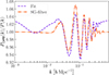 |
Fig. A.1. Comparison between the Eisenstein-Hu fitting method (in purple) and the Savitzky-Golay filter (in orange) for calculating the non-wiggle matter power spectrum. The curves show the ratio of the total linear matter power spectrum from CAMB divided by the corresponding smooth non-wiggle power spectrum. |
In Fig. A.2 we show the constraining power that comes from combining the spectroscopic GCsp and the photometric WL probes, compared to the photometric-only 3×2 pt analysis. We show this for the parameters h - log10|fR0| and for Ωb, 0, which we had omitted in previous plots. As we can see, the GCsp probe in combination with WL is crucial to break degeneracies and improve the constraints on the Hubble parameter and the baryon density fraction, thanks to its sensitivity to these parameters, especially at the scales of the BAO wigggles.
In the left panel of Fig. A.3 we show in dark yellow the fully marginalised contours for the HS7 model and in dashed cyan the contours for a ΛCDM equivalent, after fixing (maximising) the extra parameter log10|fR0|. We do this to prove that the HS7 model is close enough to ΛCDM and that we recover very similar constraints when comparing the same number of free parameters, even if the HS7 model has a larger σ8. Our results match very well those of EC20 for the same ΛCDM scenario and the same settings, when taking into account the error in the units that was present in that paper, as already mentioned in Sect. 4. In the right panel of Fig. A.3 we show the pessimistic (in cyan, empty contours) and optimistic (in orange, filled contours) settings for the full combination of photometric probes. As discussed in Sect. 5 and shown in Table 2 the pessimistic errors on log10|fR0| are about a factor 2 to 3 larger than in the optimistic setting, mainly due to the fact that non-linear scales contain crucial information on the scale-dependent growth of perturbations and the additional clustering caused by the fifth force present in f(R). This highlights the importance in the future for real-data analysis to model these scales correctly and accurately to avoid introducing systematic errors in the analysis that could severely bias the parameter determination. While extracting information from these scales will be possible, the modelling of systematics and astrophysical uncertainties is not yet at the level where we can have robust and unbiased constraints. Therefore, we have decided to use the pessimistic setting as our baseline case. The final constraints should lie somewhat in between these two limiting settings.
In Fig. A.4 we show the comparison between the settings of the Euclid spectroscopic probe as described in Table 1, for the HS6 model. In the left panel we show for the GCsp probe the pessimistic quasi-linear (dotted-dashed lines), the pessimistic (green) and the optimistic (purple) cases. One can see that, as expected, the difference between the pessimistic scale-cut at 0.25 h Mpc−1 and the optimistic one at 0.3 h Mpc−1, is not that visible in the final contours. However, the quasi-linear case (kmax = 0.15 h Mpc−1), does discard important information in the quasi-linear regime and this has a major impact on the contours, degrading them by a factor 2 or more. In the right panel of Fig. A.4 we show again the baseline pessimistic case in green and we show three further cases, which we encompass under the non-linear realistic settings. They all have a scale-cut of 0.25 h Mpc−1 as in the pessimistic setting, but with an increasing number of nuisance parameters:
-
i) In yellow shaded regions, the ‘Qbias’ case, where we vary two independent parameters A1 and A2 that account for a scale-dependent galaxy bias in modified gravity, see Eq. (26).
-
ii) In dark blue solid line contours, the ‘sigmas’ case in which we vary the σp and σv parameters independently at each of the 4 redshift bins.
-
iii) In cyan dot-dashed contours we combine cases i) and ii) for a total of 10 extra nuisance parameters compared to our baseline pessimistic setting.
Due to the increased number of parameters, we had to use the more accurate numerical derivative algorithm of a forward-4-point-stencil. We checked that using this method we recover stable results and for the other simpler cases, the changes in the Fisher matrices were negligible. As stated before, these derivative methods and the Fisher matrix pipeline are available in the publicly released Cosmicfispie code. Strikingly, the loss in constraining power between case iii) of our non-linear realistic setting and the pessimistic quasi-linear setting is similar. In the baseline pessimistic setting the percentage error on log10|fR0| is 3.9%, this increases to 4.9% in the ‘Qbias’ case i), to 5.2% in the ‘sigmas’ case ii) and to 8.0% in the third combined case iii). This value is close to the one in the pessimistic quasi-linear setting of 7.4% reported in Table 2. For the other cosmological parameters the degradation in constraints in case iii) is not that strong and they are better constrained as in the pessimistic quasi-linear case. This indicates that the Q-bias scale-dependent galaxy bias is strongly degenerate with the scale-dependent growth induced by an f(R) model.
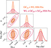 |
Fig. A.2. Joint marginal error contours at 1 σ and 2 σ on a subset of the cosmological parameters for a flat f(R) model with |fR0| = 5 × 10⁻⁶ (HS6). In solid orange the combination of GCsp and WL and in red contour lines the 3×2 pt combination of photometric probes. It can be seen that it is the spectroscopic probes driving the constraints on Ωb, 0 and h, which in combination with WL helps break degeneracies. |
Finally, in Table A.1 we list the 1 σ marginalised errors for all the other models considered in this paper, namely HS5, HS7 and the ΛCDM counterpart.
Forecast 1 σ marginal relative errors on the cosmological parameters for a flat f(R) model with |fR0| = 5 × 10⁻⁵, |fR0| = 5 × 10⁻⁷ and the flat ΛCDM model in the pessimistic and optimistic settings.
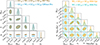 |
Fig. A.3. Left panel: Comparison of the posterior contours when fixing (i.e. maximising) the log10|fR0| parameter from the Fisher matrices for the full combination GCsp+WL+GCph+XCph for the HS7 case. In dark yellow the HS7 case and in cyan dashed lines the GR baseline case. The contour shapes match very well in all parameter subspaces, considering that in σ8 their fiducial values are different. This is expected from the fact that the HS7 model is very close to ΛCDM. Right panel: Full combination GCsp+WL+GCph+XCph for the HS6 case, comparing the optimistic (yellow, solid) and pessimistic (cyan, empty) specifications. See Table 1 for details on these settings. |
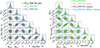 |
Fig. A.4. Left panel: Joint marginal error contours 1 σ and 2 σ on the cosmological parameters for a flat f(R) model with |fR0| = 5 × 10⁻⁶ (HS6) for the GCsp probe. In black dot-dashed lines the quasi-linear case (kmax = 0.15 h Mpc−1), in solid green the baseline pessimistic case (kmax = 0.25 h Mpc−1) and in purple the optimistic case (kmax = 0.3 h Mpc−1). Right panel: Same as in the left panel but now comparing the pessimistic baseline case (solid green) against the more realistic models, with increasing level of complexity. In yellow the addition of scale-dependent Q-bias, in dark blue the addition of free σp and σv nuisance parameters at each redshift bin and in cyan (dash-dotted line contour) the addition of both terms together for a total of 10 extra nuisance parameters. The loss in constraining power when using this more accurate model is similar to the loss in constraining power when doing a quasi-linear scale cut. |
Appendix B: Nuisance parameters
In this section we specify the nuisance parameters used in the Fisher matrix forecast analysis, both for the spectroscopic as well as for the photometric probes. These values follow closely those used in EC20. In the case of the spectroscopic survey we also specify the parameters used in the non-linear realistic scenario where we use the Q-bias approximation and the σp and σv parameters are varied. For these two, the actual nuisance parameter is one rescaling factor per redshift bin around their fiducial values, which are cosmology- and μ- (cosine of the line-of-sight angle) dependent. In the table we list their fiducial values for the HS6 model and for μ = 0.
Nuisance parameters for the photometric (top) and spectroscopic (bottom) surveys. In the spectroscopic survey, the Q-bias and the velocity dispersion parameters are only used in the fully non-linear realistic scenario.
All Tables
Forecast 1σ marginal relative errors on the cosmological parameters for a flat f(R) model with |fR0| = 5 × 10⁻⁶ (log10|fR0| = −5.301) in the pessimistic and optimistic cases using Euclid observations of spectroscopic galaxy clustering (GCsp), WL, photometric galaxy clustering (GCph), and the cross-correlation among the photometric probes XCph.
Forecast 1 σ marginal relative errors on the cosmological parameters for a flat f(R) model with |fR0| = 5 × 10⁻⁵, |fR0| = 5 × 10⁻⁷ and the flat ΛCDM model in the pessimistic and optimistic settings.
Nuisance parameters for the photometric (top) and spectroscopic (bottom) surveys. In the spectroscopic survey, the Q-bias and the velocity dispersion parameters are only used in the fully non-linear realistic scenario.
All Figures
|
Fig. 1. Relative difference between EFTCAMB and MGCAMB for the linear matter power spectrum (ΔP/P ≡ [PEFTCAMB − PMGCAMB]/PMGCAMB) at three different redshifts, z = 0 (solid orange line), z = 1 (dashed blue line), and z = 3 (dot-dashed purple line) for the three fiducial models with |fR0| = 5 × 10⁻⁵ (HS5), |fR0| = 5 × 10⁻⁶ (HS6), and |fR0| = 5 × 10⁻⁷ (HS7). |
| In the text | |
|
Fig. 2. Ratio of the scale-dependent matter growth rate f(k, z) in f(R) gravity (for the fiducial value |fR0| = 5 × 10⁻⁶) with respect to ΛCDM for three different wavenumbers, 5 × 10⁻³ (solid blue line), 5 × 10⁻² (dashed purple line), and 5 × 10⁻¹ h Mpc−1 (dot-dashed orange line), as a function of redshift from z = 0 to z = 2.5. The smaller the spatial scales and the lower the redshifts, the larger the enhancement of the growth rate compared to ΛCDM. |
| In the text | |
|
Fig. 3. Ratio of the non-linear power spectrum in f(R) gravity to ΛCDM from the fitting function in Eq. (27) for three different values of the |fR0| parameter, namely, 5 × 10⁻⁵ (blue line), 5 × 10⁻⁶ (purple line), and 5 × 10⁻⁷ (orange line), as a function of scale, k, evaluated at two different redshifts, z = 0.25 (solid lines) and z = 1.75 (dashed lines). These redshifts correspond approximately to the means of the first and last lensing tomographic bins of our survey, respectively (see Section 4). The fitting formula designed in Winther et al. (2019) is not defined outside 10−7 < |fR0| < 10−4. |
| In the text | |
|
Fig. 4. Marginalised 1σ errors on cosmological parameters relative to their corresponding fiducial value for the pessimistic baseline case, which equals to |fR0| = 5 × 10⁻⁶. We show results for GCsp (purple); WL (blue); GCsp + WL (orange); the combination of all photometric probes, including cross correlations, WL + GCph + XCph (red); and the combination of all spectroscopic and photometric probes, GCsp + WL + GCph + XCph, (yellow). One can see that the constraints on log10|fR0| and σ8 are similar among GCsp and WL, but for other parameters such as the Hubble parameter, h, or the fraction of baryons, Ωb, 0, the constraints coming from GCsp alone are even more stringent than the constraints of all photometric probes combined on their own. |
| In the text | |
|
Fig. 5. Joint marginal error contours at 1σ and 2σ on the cosmological parameters for a flat f(R) model with |fR0| = 5 × 10⁻⁶ in the optimistic setting. Purple is for GCsp, blue for WL, orange for the combination GCsp + WL, and yellow for all the photometric probes including their cross-correlation XCph, combined with GCsp, namely GCsp + WL + GCph + XCph. While the WL probe is unable to properly constrain the Hubble parameter h and the primordial slope ns on its own, the orthogonality of the contours for GCsp and WL in the subspaces involving h and ns, helps lift degeneracies and further improves the fully marginalised constraints on log10|fR0|, when probe combinations are used. |
| In the text | |
|
Fig. 6. Same as Fig. 5 (HS6) but for a subset of the cosmological parameters (omitting WL alone) when transforming the contours back into the fundamental parameter |fR0|. While in the logarithmic case the marginalised Fisher contours are simply Gaussians by definition, this is not the case for the contours on the linearly parameterised case |fR0|. For the probes GCsp (purple) and WL (blue) on their own which are less constraining, the errors on |fR0| are very asymmetric with heavy tails on the right. However, the smaller the 1σ marginalised error on log10|fR0| is, the better the marginalised posterior on |fR0| can be approximated by a Gaussian. This can be seen for the full combination of Euclid probes (yellow). |
| In the text | |
|
Fig. 7. Left: Joint marginal error contours at 1σ and 2σ on the cosmological parameters for a flat f(R) model with |fR0| = 5 × 10⁻⁶ (HS6) vs. |fR0| = 5 × 10⁻⁷ (HS7) in the pessimistic setting. Lighter colours and solid contours correspond to HS6, while darker colours and dashed empty contours correspond to HS7. In purple the spectroscopic GCsp, in red the combination of photometric probes (GCsp + WL + GCph + XCph). These two HS models only differ by their value of σ8 and log10|fR0|. Therefore the contours look very similar in the standard cosmological parameters. For log10|fR0| the ellipses become much more elongated in HS7. Right: One-dimensional fully marginalised posteriors on the |fR0| parameter for HS7 (dashed), HS6 (solid), and HS5 (dotted) after applying the transformation in Eq. (37). We use the same colour convention as before. The shaded vertical areas correspond to the 1σ confidence intervals, while the Gaussian curves extend up to 3σ. Using the full combination of photometric probes, HS7 and HS6 can be distinguished at 2σ, and both of them can be distinguished from HS5 at 3σ or more. |
| In the text | |
|
Fig. A.1. Comparison between the Eisenstein-Hu fitting method (in purple) and the Savitzky-Golay filter (in orange) for calculating the non-wiggle matter power spectrum. The curves show the ratio of the total linear matter power spectrum from CAMB divided by the corresponding smooth non-wiggle power spectrum. |
| In the text | |
|
Fig. A.2. Joint marginal error contours at 1 σ and 2 σ on a subset of the cosmological parameters for a flat f(R) model with |fR0| = 5 × 10⁻⁶ (HS6). In solid orange the combination of GCsp and WL and in red contour lines the 3×2 pt combination of photometric probes. It can be seen that it is the spectroscopic probes driving the constraints on Ωb, 0 and h, which in combination with WL helps break degeneracies. |
| In the text | |
|
Fig. A.3. Left panel: Comparison of the posterior contours when fixing (i.e. maximising) the log10|fR0| parameter from the Fisher matrices for the full combination GCsp+WL+GCph+XCph for the HS7 case. In dark yellow the HS7 case and in cyan dashed lines the GR baseline case. The contour shapes match very well in all parameter subspaces, considering that in σ8 their fiducial values are different. This is expected from the fact that the HS7 model is very close to ΛCDM. Right panel: Full combination GCsp+WL+GCph+XCph for the HS6 case, comparing the optimistic (yellow, solid) and pessimistic (cyan, empty) specifications. See Table 1 for details on these settings. |
| In the text | |
|
Fig. A.4. Left panel: Joint marginal error contours 1 σ and 2 σ on the cosmological parameters for a flat f(R) model with |fR0| = 5 × 10⁻⁶ (HS6) for the GCsp probe. In black dot-dashed lines the quasi-linear case (kmax = 0.15 h Mpc−1), in solid green the baseline pessimistic case (kmax = 0.25 h Mpc−1) and in purple the optimistic case (kmax = 0.3 h Mpc−1). Right panel: Same as in the left panel but now comparing the pessimistic baseline case (solid green) against the more realistic models, with increasing level of complexity. In yellow the addition of scale-dependent Q-bias, in dark blue the addition of free σp and σv nuisance parameters at each redshift bin and in cyan (dash-dotted line contour) the addition of both terms together for a total of 10 extra nuisance parameters. The loss in constraining power when using this more accurate model is similar to the loss in constraining power when doing a quasi-linear scale cut. |
| In the text | |
Current usage metrics show cumulative count of Article Views (full-text article views including HTML views, PDF and ePub downloads, according to the available data) and Abstracts Views on Vision4Press platform.
Data correspond to usage on the plateform after 2015. The current usage metrics is available 48-96 hours after online publication and is updated daily on week days.
Initial download of the metrics may take a while.