| Issue |
A&A
Volume 707, March 2026
|
|
|---|---|---|
| Article Number | A246 | |
| Number of page(s) | 9 | |
| Section | Astrophysical processes | |
| DOI | https://doi.org/10.1051/0004-6361/202554646 | |
| Published online | 09 March 2026 | |
Misalignment of the Lense-Thirring precession by an accretion torque
1
Department of Astronomy, Astrophysics & Space Engineering, Indian Institute of Technology Indore, Simrol Indore 453552 Madhya Pradesh, India
2
Center for Interdisciplinary Exploration & Research in Astrophysics (CIERA), Physics & Astronomy, Northwestern University Evanston IL 60202, USA
3
Astronomical Institute, Academy of Sciences Boční II 141 31 Prague 4, Czech Republic
4
Nicolaus Copernicus Astronomical Center ul. Bartycka 18 PL 00-716 Warsaw, Poland
5
Department of Physics and Astronomy, College of Charleston 66 George St Charleston SC 29424, USA
6
Center for Computational Astrophysics, Flatiron Institute 162 5th Avenue New York NY 10010, USA
★ Corresponding authors: This email address is being protected from spambots. You need JavaScript enabled to view it.
; This email address is being protected from spambots. You need JavaScript enabled to view it.
; This email address is being protected from spambots. You need JavaScript enabled to view it.
Received:
19
March
2025
Accepted:
30
November
2025
Abstract
Context. Orbiting matter misaligned with a spinning black hole undergoes Lense-Thirring precession due to the frame-dragging effect. This phenomenon is particularly relevant for type-C QPOs observed in the hard states of low-mass X-ray binaries. However, the accretion flow in these hard states is complex, consisting of a geometrically thick, hot corona surrounded by a geometrically thin, cold disk. Recent simulations demonstrate that, in such a truncated disk scenario, the precession of the inner, hot corona slows due to its interaction with the outer, cold disk.
Aims. This paper aims to provide an analytical description of the precession of an inner (hot) torus in the presence of accretion torques exerted by the outer (cold) disk.
Methods. Using the angular momentum conservation equation, we investigated the evolution of the torus angular momentum vector for various models of accretion torque.
Results. We find that, in general, an accretion torque tilts the axis of precession away from the black hole spin axis. In all models, if the accretion torque is sufficiently strong, it can halt the precession; any perturbation from this stalled state causes the torus to precess around an axis that is misaligned with the black hole spin axis.
Conclusions. The accretion torque exerted by the outer thin disk can cause precession around an axis that is neither aligned with the black hole spin axis nor perpendicular to the plane of the disk. This finding may have significant observational implications, as the jet direction, if aligned with the angular momentum axis of the torus, may no longer reliably indicate the black hole spin axis or the orientation of the outer accretion disk.
Key words: black hole physics / relativistic processes / X-rays: binaries
© The Authors 2026
 Open Access article, published by EDP Sciences, under the terms of the Creative Commons Attribution License (https://creativecommons.org/licenses/by/4.0), which permits unrestricted use, distribution, and reproduction in any medium, provided the original work is properly cited.
This article is published in open access under the Subscribe to Open model. This email address is being protected from spambots. You need JavaScript enabled to view it. to support open access publication.
1. Introduction
Quasiperiodic oscillations (QPOs) in the X-ray light curves of accreting black hole and neutron star X-ray binary systems, characterized by broad peaks in their power spectra, are a characteristic feature of these systems (see van der Klis 2006; Remillard & McClintock 2006, for reviews). The “quasiperiodic” nature arises from the modulation of either the frequency or the amplitude of the light curves. Quasiperiodic oscillations offer a unique opportunity to study the strong gravitational fields surrounding compact objects, providing insights into physical processes on spatial scales that are otherwise inaccessible, with the exception of nearby supermassive black holes observed by the Event Horizon Telescope. Based on their frequency, black hole QPOs are typically categorized as either high frequency (≥60 Hz) or low frequency (≤30 Hz) (Psaltis et al. 1999; Ingram & Done 2011).
In addition to rapid variability, accreting black hole X-ray binaries exhibit spectral state transitions over periods ranging from days to months (e.g. Homan & Belloni 2005; Corral-Santana et al. 2016; Singh et al. 2019). These transitions, often depicted as q-shaped tracks in hardness-intensity diagrams, reflect significant changes in the geometry and physical conditions of the accretion flow (Fender et al. 2004; Belloni et al. 2005; McClintock & Remillard 2006; Weng et al. 2021). The primary spectral states are classified as “soft” and “hard,” though intermediate states have also been observed (Belloni 2010; Done et al. 2007). In the soft state, the X-ray spectrum is dominated by thermal emission, which resembles blackbody radiation from a cool, optically thick, geometrically thin accretion disk (Shakura & Sunyaev 1973). In contrast, the hard state is dominated by nonthermal, power-law emission produced by Compton up-scattering of soft seed photons from the disk by a hot, optically thin electron cloud, commonly referred to as the “corona” (Haardt & Maraschi 1991, 1993; Zdziarski et al. 1998; Zdziarski & Gierliński 2004; Fabian et al. 2000; Krawczynski & Beheshtipour 2022; Grošelj et al. 2024).
While the precise geometry of the corona remains uncertain, a widely accepted model envisions a truncated disk, where the inner thin disk is replaced by a corona (Esin et al. 1997; Done et al. 2007). As the system evolves from the hard to the soft state, the disk migrates inward and the corona collapses, eventually reaching the innermost stable circular orbit (Plant et al. 2015; Kara et al. 2019; Buisson et al. 2019; De Marco et al. 2021; Rawat et al. 2025).
Quasiperiodic oscillations are observed across different spectral states, with low-frequency QPOs (LFQPOs) being particularly prominent (Wijnands & van der Klis 1999; Casella et al. 2005). Type-A and type-B LFQPOs typically appear during transitions through the intermediate states toward the soft state, whereas type-C LFQPOs appear mostly in the hard state. High-frequency QPOs, on the other hand, tend to occur in high-luminosity accretion states (Remillard et al. 2002). Several models attribute QPOs to oscillations in the corona or the thin disk, or to waves generated by instabilities within the accretion flow1. Understanding the origin and mechanisms driving QPOs may be helpful in constraining the geometry and location of the corona.
One of the most common interpretations of the type-C LFQPO is that it results from Lense-Thirring precession of the corona. This hypothesis is supported by observations showing that the QPO amplitude and phase lag between hard and soft photons, measured at the QPO frequency, are strongly dependent on the inclination angle of the system (Motta et al. 2015; van den Eijnden et al. 2017). In the truncated-disk model, the precession of the corona, surrounded by the truncated disk, produces the type-C LFQPOs (Ingram et al. 2009; Ingram & Done 2011). This model also explains the observed correlation between the low-frequency break (attributed to the viscous timescale at the transition radius) and the type-C QPO frequency (attributed to the precession frequency of the inner hot flow) in the power spectra of accreting black hole systems. The model has been further explored in great detail to include time-dependent emission of iron-line profiles arising from the variable orientation of the hot inner flow and the outer thin disk with respect to the observer (Ingram & Done 2012b; Ingram et al. 2016), correlation of the X-ray (Zycki et al. 2016) and optical (Veledina & Poutanen 2015) spectral properties with QPO phase, as well as variable X-ray polarization (Ingram et al. 2015; Fragile et al. 2025).
A sufficiently hot orbiting fluid around a Kerr black hole may take the shape of a torus. Among the eigenmodes of this torus (assuming it is slender) are rigid-body motions, the simplest being a uniform vertical2 oscillation at a frequency corresponding to the vertical epicyclic frequency of a test particle, σ = ω⊥ (Bursa et al. 2004). This eigenmode is often invoked to explain high-frequency QPOs observed in X-ray binaries. This mode, characterized by identical vertical displacements of all fluid elements, corresponds to the m = 0 mode in a more general class of motions, where vertical displacement varies azimuthally as exp(imϕ). The pattern frequency of these oscillations3 is given by ωp = (σ + mΩ)/m, where Ω is the orbital frequency. The m = −1 mode, in particular, corresponds to a rigid-body precession of an inclined torus at a frequency defined by the difference between the orbital and vertical epicyclic frequencies,
 (1)
(1)
This precession mechanism can be understood by considering the orbit of a test particle inclined at an angle to the equatorial plane of the black hole. Due to the frame-dragging effect of the spinning black hole, the orbit undergoes nodal precession, known as Lense-Thirring precession (Lense & Thirring 1918). The vertical, epicyclic, rigid-body mode is therefore thought to explain both the high- and low-frequency QPOs (for m = 0 and m = −1, respectively) observed in X-ray binaries. (A similar combination of the radial epicyclic and orbital frequencies was suggested as an explanation for kilohertz QPOs in neutron stars by Stella & Vietri 1998; Stella et al. 1999).
A torus with substantial radial extent can also undergo nearly rigid-body precession if the sound travel time across the torus is shorter than the precession period, 2π/ωp. In this case, the Lense-Thirring torque is efficiently communicated through bending waves, causing the torus to behave as a solid body (Papaloizou & Terquem 1995; Lodato & Facchini 2013; Nixon & King 2016). The precession periods of non-slender tori were derived analytically using perturbative expansions of the fluid equations (Blaes et al. 2007) (see also Straub & Šrámková 2009, for a full general relativistic treatment), and these precession frequencies match the form of Equation (1), with radial averages replacing the orbital and vertical frequencies (Blaes et al. 2007).
Numerous general relativistic magneto-hydrodynamic (GRMHD) simulations confirmed the robustness of such a nearly rigid-body Lense-Thirring precession of accreting tori (Fragile & Anninos 2005; Fragile et al. 2007; Morales Teixeira et al. 2014; Liska et al. 2018). In particular, Fragile et al. (2007) showed that the numerically derived precession rates agree well with the precession frequency for a rigid body (Liu & Melia 2002). Their derived expression for the precession frequency is a function of the inner and outer radii of the torus, based on the density and rotation profiles extracted from their simulations. These formulas have since been refined by Ingram et al. (2009), Ingram & Done (2011, 2012a) and De Falco & Motta (2018).
In the case of free Lense-Thirring precession, the “tilt” angle between the axes of the torus and the black hole remains constant over time. This means that the angular momentum vector of the torus rotates uniformly about the black hole spin axis, sweeping out a conical surface.
However, in an astronomical context, the torus is typically the inner region of an accretion flow, surrounded by a disk. Notably, none of the studies listed above account for the effect of the outer disk on the torus precession. Recent GRMHD simulations of tilted and truncated accretion disks with inner tori demonstrate that the exchange of angular momentum between the outer thin disk and the torus introduces an accretion torque, which significantly alters the torus precession dynamics (Bollimpalli et al. 2023).
In this paper, we analytically examine the leading effects of an accretion torque on the Lense-Thirring precession of an inner torus within this theoretical context. We find that the torus precesses around an axis different from the black hole spin axis. In other words, the precession occurs around an axis that is neither aligned with the black hole spin axis nor perpendicular to the plane of the accretion disk. This finding has important observational implications: if the jet is anchored in the torus and shares its mean angular-momentum axis, the jet itself need not be aligned with the black hole spin. Recent Imaging X-ray Polarimetry Explorer (IXPE) observations showing X-ray polarization roughly aligned with the jet direction (Krawczynski & Beheshtipour 2022; Zdziarski et al. 2023) suggest a common corona–jet axis, but this axis does not necessarily coincide with the spin. This scenario favors jet formation mechanisms influenced by the accretion flow (e.g., Blandford & Payne 1982, or hybrid models), while a pure Blandford & Znajek (1977) jet anchored strictly to the horizon would instead align with the spin. However, rapid precession of the torus or small-scale jet wobbling could make these effects difficult to detect observationally. Additionally, magnetic topology or GRMHD effects could further modulate the effective jet axis.
The rest of the paper is organized as follows: In Sect. 2, we present the basic framework of our model, which is based on the truncated disk geometry. Sect. 3 derives the general solution for the precession of a tilted, accreting torus. In Sect. 4, we provide specific examples of different accretion torques and demonstrate how precession occurs in each case. Sect. 5 compares our results with recent simulation findings from Bollimpalli et al. (2023). Finally, in Sect. 6, we discuss the observational implications and present our conclusions.
2. The overall picture
We consider a spinning black hole with its axis misaligned with respect to the accretion flow, adopting a two-component accretion flow geometry that is thought to be relevant for hard states of low-mass X-ray binaries (LMXBs): an inner hot torus surrounded by an outer cool, thin disk, as shown in Fig. 1. Since the inner torus is geometrically thick and optically thin, bending waves are communicated efficiently enough for the torus to precess as a rigid body4. In contrast, due to the geometrically thin and optically thick nature of the outer disk, the bending waves are diffused away there, and we expect no precession in this region.
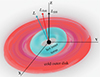 |
Fig. 1. Geometry of our model. The direction of the black-hole angular momentum (LBH) coincides with the z-direction of the Cartesian system used in the calculations. Due to misalignment with the black-hole spin, the angular momenta of the outer thin accretion disk (Ldisk) and inner hot torus (L) have nonzero projections onto the x-y plane. |
The accretion flow is tilted such that if we align the z axis of a Cartesian coordinate frame with the spin axis of the black hole (the “vertical” direction; see Fig. 1), the angular momentum vector of the disk has a nonzero projection onto the x-y plane. Thus, any accretion from the disk onto the torus tends to change the x-y component of the torus angular momentum through the advection of the angular momentum of the disk (in addition to affecting the z component). This results in rotation in the x-y plane of the angular momentum projection, beyond any relativistic precession, if the torus is already tilted with respect to the black hole spin axis. Alternatively, it tilts the torus if the torus is aligned with the black hole. The net advection rate of the angular momentum in the torus is equivalent to a torque, which we refer to as the accretion torque. We aimed to derive the time evolution of the angular momentum of the torus for a given accretion torque and, in particular, to determine the direction in which the torus axis points. More specifically, we were interested in the evolution of the precession angle of the torus, defined as the angle from the x axis to the x-y projection of the torus angular momentum vector.
3. The torque equation
For our purposes, it was sufficient to use a Newtonian equation of angular momentum conservation,
 (2)
(2)
with τ = τp + τacc. We included the main effect of general relativity by adopting a Lense-Thirring torque,
 (3)
(3)
where ωp = 2(G/c2)(LBH/R3) is a constant vector in the vertical (black hole spin) direction, LBH is the black hole angular momentum, and R is a torus mean radius (Wilkins 1972; Bardeen & Petterson 1975). In effect, we assumed that the torus had a constant free precession rate, ωp, regardless of its mass and total angular momentum L. The second component of the torque, τacc, is the accretion torque, equal to the net rate of angular momentum advection. Thus, the evolution of the torus angular momentum is given by
 (4)
(4)
We ignored the viscous terms in the above conservation equation, as they were found to be negligible compared to the Lense-Thirring torque and the angular momentum fluxes in the simulations of Bollimpalli et al. (2023).
In the Cartesian coordinate system introduced in the previous section,  , and hence τp does not depend on Lz. Therefore, the z component of the torque equation,
 (5)
(5)
does not couple to the x and y components; our analysis focuses on the latter. Introducing complex variables,
 (6)
(6)
so that Lx = Re L, Ly = Im L, and similarly for τacc, we can rewrite the x and y components of Eq. (4) as
 (7)
(7)
For τacc = 0 the equation has a simple solution corresponding to uniform rotation in the positive direction,
 (8)
(8)
This represents the x-y projection of the angular momentum vector of the torus undergoing Lense-Thirring free precession, hence the notation.
The precession may be halted for a sufficiently large accretion torque (or a sufficiently small tilt angle of the torus). It suffices that the following equation be satisfied, starting at some instant t0:
 (9)
(9)
for dL/dt = 0 to hold for t > t0. In the x-y plane, this is just
 (10)
(10)
and has a simple interpretation. The Lense-Thirring torque is perpendicular to the angular momentum vector and leads it in phase by π/2 (corresponding to a factor of i). An accretion torque of equal magnitude but opposite direction counteracts this effect; it is also perpendicular to the angular momentum vector, but lags it by the same phase angle, π/2 (corresponding to a factor of −i).
However, this equilibrium point, denoted as L1, corresponding to τacc = τ1, is not stable: a small fluctuation of L leads to the resumption of precession (about the equilibrium point L1). Indeed, keeping τ1 = −iωpL1 fixed, a change of L from L1 to L2 at time t2 leads to the resumption of precession for t > t2 with L0 = L2 − L1 (Eqs. (7), (8), (10)). We obtained a similar result following an impulsive change in the accretion torque, τacc, from τ1 to τ2. The precession now occurs around the equilibrium point L2 = iτ2/ωp with amplitude L0 = L1 − L2. This is a generic result: a change in the accretion torque changes the precession and can induce a Lense-Thirring precession where none had occurred before, as discussed in Subsection 4.3.
The general solution of the inhomogeneous linear differential Eq. (4) is the sum of the general solution of the homogeneous equation
 (11)
(11)
which is LLT(t), and a particular solution of the inhomogeneous Eq. (4). Thus,
 (12)
(12)
where  is a particular solution that satisfies
 (13)
(13)
To summarize, the general solution for the motion of a tilted accreting torus is a precession (Eq. (8)) at the Lense-Thirring frequency around a possibly moving axis,  . This axis is determined by the solution of Eq. (13), which can be written as
 (14)
(14)
We present the determination of  and L(t) for any given τacc(t) in the next section.
4. Solutions
We now present the solutions to Eq. (13) for four simple forms of τacc. In steady state, the net rate of angular momentum advection can be assumed to be constant in time. This corresponds to a steady torque (see Sect. 4.1). By contrast, the luminosity of X-ray binaries often varies over time. A steady rise in the advected angular momentum rate (Sect. 4.2) may correspond to black hole disks going into “outburst.” A change of the accretion torque from one value to another (see Sect. 4.3) could model state transitions of black hole binaries, or the torque could oscillate (Sect. 4.4). Finally, the ring of the accretion disk directly adjacent to the torus may itself precess, for instance, in the corrugation mode of diskoseismology (Kato 1989; Silbergleit et al. 2001; Kato 1993; Ipser 1996). The x-y components of the advected angular momentum could then vary harmonically, so that the accretion torque could be taken to rotate at a definite frequency (Sect. 4.5).
4.1. Steady accretion torque
For a steady torque, τacc = τf = const, the solution is
 (15)
(15)
The general solution of Eq. (7) is then
 (16)
(16)
describing precession at the Lense-Thirring frequency about a point (in the x-y plane) which is advanced by π/2 in phase with respect to the accretion torque (see Fig. 2). We explain the reason for this in the paragraph following Eq. (10). The amplitude of precession, L0, is given by the initial conditions.
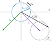 |
Fig. 2. Precession of the angular momentum vector (L) of the inner torus when a steady accretion torque τf = τA is applied. This figure is projected into the plane perpendicular to the black-hole spin. In the absence of an accretion torque, the angular momentum vector executes free Lense-Thirring precession, LLT(t), around the direction of the black hole spin. When the torque is applied, the general solution consists of free Lense-Thirring precession about a new direction, shifted by a constant, |

4.2. Linearly growing torque
Taking τacc(t) = τ0 + (t/tf)τf, we obtain
 (17)
(17)
Here, the x-y projection of the tip of the angular momentum vector undergoes uniform circular motion at the Lense-Thirring precession rate, similar to the case in Section 4.1. However, in this scenario, the point around which this precession occurs experiences a linear drift in the direction that advances the accretion torque by π/2 in phase. In the limit of slow growth, ωptf ≫ 1, this tends to the steady torque solution, albeit with a varying position of the center of precession,  .
.
4.3. Change of torque
For an exponentially varying torque from τi to τf, with a decay constant ωh,
 (18)
(18)
In this case, the particular solution takes the form
![Mathematical equation: $$ \begin{aligned} \begin{aligned} \hat{L}(t)&= -\frac{\omega _\mathrm{h} }{\omega _{\rm p}^2+\omega _\mathrm{h} ^2}\left({{\tau _\mathrm{i} }-\tau _\mathrm{f} }\right)\exp (-\omega _\mathrm{h} t) \\&\quad +\,\mathrm{i} \left[\frac{\tau _\mathrm{f} }{\omega _{\rm p}}\,+ \frac{\omega _{\rm p}}{\omega _{\rm p}^2+\omega _\mathrm{h} ^2}\left({\tau _\mathrm{i} }-{\tau _\mathrm{f} }\right)\exp (-\omega _\mathrm{h} t)\right]. \end{aligned} \end{aligned} $$](/articles/aa/full_html/2026/03/aa54646-25/aa54646-25-eq25.gif) (19)
(19)
This solution tends exponentially to the constant torque solution. When the change is slow, ωh ≪ ωp, this approximates the steady torque solution, with a different value of the accretion torque at each instant of time:  . In the opposite limit of fast healing, ωp ≪ ωh, the solution is very close to the steady torque solution with the final value of the torque,
  .
.
A general solution consists of a free Lense-Thirring precession (8) and the special solution (19), whose properties were discussed above. Figure 3 shows two examples of how the torus angular momentum evolves for the slow (ωh = 0.2ωp; left panel) and fast (ωh = 2ωp; middle panel) change of the accretion torque from 0 to τf. Since the accretion torque is initially zero, the torus precesses around the z-axis. Interestingly, even if the initial torus is aligned with the black hole spin axis, i.e., if precession is zero, the accretion torque change can still excite free precession of the torus, as shown in the last panel of Fig. 3.
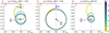 |
Fig. 3. Trajectory of the torus angular-momentum vector in the x-y plane when the accretion torque evolves exponentially from zero to τf = −1 for various cases. A torus that is initially precessing with an angular momentum L(0) = − 0.3i approaches the final state of precession about the new equilibrium point, iτf/ωp, slowly or rapidly for a low (ωh = 0.2ωp) or high (ωh = 2ωp) healing frequency, as in the left and middle panels, respectively. The right panel presents the same case as in the left panel (i.e., ωh = 0.2ωp), except that initially the torus has a zero angular momentum projection onto the x-y plane, i.e., L(0) = 0, highlighting that a change in accretion torque can induce precession in a torus. In all three examples, we set ωp = 1 and the phase evolution is represented by both the color and the decreasing thickness of the curve. |
4.4. Oscillating torque
None of the three simple torque models in Sections 4.1, 4.2, and 4.3 provide an adequate description of the simulations of Bollimpalli et al. (2024). One may similarly consider a change in torque that oscillates between τA and τB at a frequency ωh:
 (20)
(20)
For this torque, the particular solution consists of two perpendicular oscillations of the angular momentum vector in the x-y plane,
![Mathematical equation: $$ \begin{aligned} \begin{aligned} \hat{L}(t)&= \frac{\omega _\mathrm{h} }{\omega _{\rm p}^2-\omega _\mathrm{h} ^2}\frac{\left({{\tau _\mathrm{B} }-\tau _\mathrm{A} }\right)}{2}\cos (\omega _\mathrm{h} t) \\&\quad +\,\mathrm{i} \left[\frac{\left({{\tau _\mathrm{A} }+\tau _\mathrm{B} }\right)}{2\omega _{\rm p}}\,+ \frac{\omega _{\rm p}}{\omega _{\rm p}^2- \omega _\mathrm{h} ^2}\frac{\left({\tau _\mathrm{B} }-{\tau _\mathrm{A} }\right)}{2}\sin (\omega _\mathrm{h} t)\right]. \end{aligned} \end{aligned} $$](/articles/aa/full_html/2026/03/aa54646-25/aa54646-25-eq29.gif) (21)
(21)
As the two oscillations have the same frequency but different amplitudes, the tip of the angular momentum vector traces an ellipse. As discussed in Sect. 5, this dynamic agrees well with the late time evolution of the torus angular momentum observed in numerical simulations.
4.5. Rotating torque
As a final case, we consider a rotating torque given by τacc(t) = τfexp(iω1t). The particular solution then takes the form
 (22)
(22)
and the general solution, using Eqs. (12) and (8), then reads
 (23)
(23)
This solution exhibits resonance at ω1 = ωp. As ω1 → ωp, the x-y component of the angular momentum vector L increases significantly in magnitude, implying that the torus approaches a position in which it “stands on its edge”, i.e., the plane of the torus approaches a vertical position (the torus axis becomes horizontal, i.e., aligning with the black-hole equatorial plane). An observer at infinity along the black hole axis would then see a constant aspect of the torus (no luminosity variation) during precession, while a distant observer in the equatorial plane of the black hole would presumably report large luminosity variations, seeing the torus edge-on every half precession period and face-on a quarter of a period later.
The most interesting situation occurs when the two frequencies are close, but not exactly equal, and the amplitudes of both exponentials in Eq. (23) are comparable, i.e., ω1 ≈ ωp, but ω1 ≠ ωp, and |L0|=|τf|/(ωp − ω1). Then the general solution of Eq. (12), using Eqs. (8) and (22), exhibits beats in which the amplitude of the x-y component of the angular momentum vector is modulated at the slow frequency (ωp − ω1)/2, while precessing at the fast frequency of (ω1 + ωp)/2. This modulation means that the midplane of the torus oscillates between a vertical and a horizontal position, at a frequency of (ωp − ω1). An example is shown in Fig. 4.
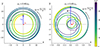 |
Fig. 4. Trajectory of the torus angular momentum vector in the x-y plane for an accretion torque rotating with frequency ω1 = 0.9ωp (left panel) and ω1 = 0.65ωp (right panel). In both cases, we use L(0) = 7i, τA = 1, and ωp = 1. The phase of the trajectory is represented by both the color and the decreasing thickness of the curve, with the starting point at t = 0, and a point later in time t marked by a circle and a triangle, respectively (for visualization purposes). The torus precesses around the black hole axis with a frequency of (ωp + ω1)/2. Additionally, the tilt angle between the black hole and torus oscillates with frequency (ωp − ω1). |
5. Comparison with simulations
Lense-Thirring precession of the inner torus is a widely accepted model for explaining type-C low-frequency QPOs typically observed in the hard or hard-intermediate states of LMXBs. Measurements of the type-C QPO frequency are often used to constrain the torus size and the black hole parameters, neglecting the outer thin disk and assuming that the torus precesses at the free Lense-Thirring frequency. However, simulations by Bollimpalli et al. (2023) demonstrate that the outer thin disk can significantly impact the torus precession rate. Motivated by these findings, we analytically explored the effect of an accretion torque using simplified forms that mimic various astrophysical scenarios. We validated our model using data from simulation a9b15L4, originally described in Bollimpalli et al. (2023), which we extended to twice the duration initially reported in that work. The initial setup of this simulation features a torus extending up to 15 GM/c2 and surrounded by a thin slab of gas, both initially misaligned with the black hole spin axis by 15°. Further details of this simulation can be found in Bollimpalli et al. (2023, 2024).
During the initial phase of the simulation (up to ∼25 000 GM/c3), as originally reported in Bollimpalli et al. (2023), the accretion torque and the Lense-Thirring torque are comparable in magnitude, as shown in the first panel of Fig. 5. For these calculations, the accretion torque was evaluated from the angular momentum accretion rate at the outer edge of the torus (r = 15 GM/c2), while the Lense-Thirring torque was computed as a volume integral of ωp(r)×L(r) over the entire volume of the torus (5 − 15 GM/c2).
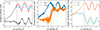 |
Fig. 5. Comparison of our model with the simulation data of Bollimpalli et al. (2024). In the left panel, we show the magnitude of the accretion (dashed, fluctuating curve) and Lense-Thirring (smooth, solid curve) torques integrated over the torus region, i.e., 5–15 GM/c2. The difference between the two magnitudes (dotted, black curve) remains close to zero in the initial phase of the simulation, up to ∼25 000 GM/c3. The middle panel shows the x and y components of the net accretion torque on the torus (solid curves) and their respective fits using Eq. (20) (dashed curves). Finally, the right panel shows the x and y components of the total angular momentum of the torus (solid curves) and their respective fits using Eq. (21) (dashed curves). The vertical dashed black lines in all panels indicate the stop time of the original simulation. |
As the simulation proceeds past the end point of the original run and into the extended run time presented here, the torus and the accretion torques begin to satisfy Eq. (4) of our model (a detailed discussion of the precession in the simulation is presented in the Appendix). During this phase (i.e., t ≳ 25 000 GM/c3), the x and y components of the accretion torque exhibit oscillatory behavior, as shown by the solid curves in the second panel of Fig. 5. The oscillatory nature of the torque likely arises from the differential precession of the transition region between the outer thin disk and the torus as the simulation evolves. We employed the oscillating torque model described in Section 4.4 to fit the accretion torque exerted on the torus region (5 − 15 GM/c2). The second panel of Fig. 5 shows the best-fit results, using Eq. (20). The best fit yields a constant ωh ≈ 0.0005, while ωp is taken to be the angular-momentum-weighted average of the Lense-Thirring precession frequency for a rigid body (see Eq. 15 of Ingram & Motta 2019),
 (24)
(24)
where the local precession frequency ΩLT = Ω − ω⊥ is given by the difference between the orbital and vertical epicyclic frequencies:
 (25)
(25)
This is the Lense-Thirring precession frequency of a test particle, and a = 0.9M and M are the spin and mass of the black hole, respectively. We directly inferred the radial profile of the time-averaged surface density, Σ, from the simulation. Subsequently, we used the best-fit values for τA and τB from Eq. (21) to compute the x and y components of the total angular momentum L, which are shown in the third panel of Fig. 5.
This exercise underscores the significant influence of the outer thin disk on both the precession rate and the axis of precession. It appears that the phase of precession initially reported in Bollimpalli et al. (2023) was transient. The later oscillatory behavior highlighted in this section could also be transient; bending waves excited in the inner region propagate outward, inducing precession in the outer thin disk for a brief period before dissipating as they diffuse away. However, since the angular momentum from this region eventually reaches the inner torus, it must impact the precession. To better understand these intricate dynamics, our future work will include running more simulations over longer periods.
6. Discussion and conclusions
The two-component model, in which an inner hot, geometrically thick accretion flow forms a torus-like structure surrounded by a cold standard accretion disk, is a popular framework for explaining the rich phenomenology of accreting black holes in low-mass X-ray binaries. For instance, the photon spectrum may be fitted by a thin accretion disk truncated at a given radius, together with a hotter component identified with the inner torus. Regarding the observed X-ray variability, the highest frequency QPOs may be explained by the m = 0 vertical epicyclic mode of the torus (Bursa et al. 2004), while the type-C QPO may correspond to the m = −1 vertical epicyclic mode (Blaes et al. 2006; Fragile et al. 2016). Numerous numerical simulations demonstrate that the free torus responds to the Lense-Thirring torque exerted by a black hole by precessing as a rigid body, provided that the sound crossing time remains short compared to the precession period (Fragile et al. 2007; Liska et al. 2018). However, in reality, the two components interact, so that free precession does not correctly describe the motion of the torus.
In a recent simulation in which a torus was placed at the center of a truncated disk, its precession acquired a seemingly complicated character. When considered to be moving about the black hole axis, the torus initially precessed at the Lense-Thirring frequency but subsequently slowed down its precession and eventually appeared to stall. The analytic model we present here does not explain this portion of the simulation. A plausible explanation is that the simulation required more time to adjust from its very artificial initial conditions.
Subsequently, however, the torus symmetry axis began to execute small loops about the stalled position. We argue that this behavior can be understood with the simple rigid-body mechanical model given in Eq. (4), once the angular momentum accreted with matter from the outer cold disk is taken into account. This additional angular momentum flux corresponds to a new source term (an accretion torque) in the angular momentum conservation equation. This paper examines the precession of the inner torus in several natural situations corresponding to different prescribed accretion torques. The solutions above describe precession around an axis that itself executes a definite motion. In general, the precession rate of the torus is itself quite robust and remains unaffected by the accretion torque, whereas the torque strongly impacts the precession amplitude, as well as on the precession axis, or the mean orientation (tilt angle time-averaged over the precession period) of the torus.
Even the simplest case of a constant (steady) accretion torque, described in Sect. 4.1, yields interesting results. In this case, the inner torus still precesses at the Lense-Thirring frequency; however, the mean direction of the angular momentum vector corresponds neither to the black hole spin nor to the orientation of the outer disk. Instead, it results from the balance between the Lense-Thirring torque τp and the accretion torque τf applied by the outer disk, and the angle between the mean direction of the torus axis and the black hole spin is ![Mathematical equation: $ \beta(t) = \arctan[|\hat L|/L_z(t)] $](/articles/aa/full_html/2026/03/aa54646-25/aa54646-25-eq34.gif) , where
, where  is the (constant) projection onto the x-y plane of the angular momentum vector, as determined by the accretion torque, cf. Eq. (15).
We also considered three situations in which the accretion torque changes gradually over time (Sects. 4.2, 4.3, and 4.4). In all cases, a slow “adiabatic” change of torque leads to a sequence of steady precession states: on top of a free Lense-Thirring precession, which remains unaffected, the mean direction of the torus angular momentum gradually changes according to the instant accretion torque. An interesting effect occurs when the rate of torque change becomes comparable to, or exceeds, the magnitude of the precession period, i.e., when (dτacc/dt)≥𝒪(ωp)τacc. The inner torus responds to these changes by increasing or decreasing the precession amplitude (depending on the relative orientation of the torus angular momentum and the torque change), in addition to the gradual change of the mean tilt angle of the torus (see Fig. 3). As noted above, state transitions in black hole LMXBs are likely accompanied by changes in the overall geometry of the accretion flow, and it is therefore natural to assume that the torque exerted by the outer accretion disk on the inner torus changes as well. Our results show that these changes may even occasionally amplify the Lense-Thirring precession of the inner flow.
Finally, we studied situations in which the accretion torque changes periodically in time (Sect. 4.5). This may occur when surrounding regions of the outer disk undergo periodic changes, either due to the presence of trapped, low-frequency oscillation modes (e.g., corrugation mode) or when the accretion rate is modulated periodically. In that case, the torque equation takes the form of a forced linear oscillator. The resonance, which occurs when the accretion torque frequency matches the precession rate of the inner torus, strongly enhances the inclination of the torus with respect to the black hole spin. Near the resonance, the torus undergoes low-frequency inclination changes in addition to its precession.
Our findings may have important implications for models of correlations between the spectral properties of black hole LMXBs and the phase of type-C QPOs. Although the precession rate of the inner flow may still equal the Lense-Thirring precession frequency, its radiation may illuminate the outer accretion disk differently than expected, leading to modified reflection spectra (Ingram & Done 2012b; Ingram et al. 2016) and polarization (Ingram et al. 2015; Fragile et al. 2025). This possibility deserves further study.
Acknowledgments
Part of this work was supported by the German Deutsche Forschungsgemeinschaft, DFG project number Ts 17/2–1. Research supported in part by by the Polish NCN grant No. 2019/33/B/ST9/01564. DAB acknowledges support from IIT-Indore, through a Young Faculty Research Seed Grant (project: ‘INSIGHT’; IITI/YFRSG/2024-25/Phase-VII/02). JH acknowledges support of the the Czech Science Foundation (GAČR) grant No. 21-06825X. PCF gratefully acknowledges the support of NASA through award No 23-ATP23-0100. The Flatiron Institute is a division of the Simons Foundation.
References
- Bardeen, J. M., & Petterson, J. A. 1975, ApJ, 195, L65 [Google Scholar]
- Belloni, T. 2010, The Jet Paradigm (Berlin: Springer Verlag), 794 [Google Scholar]
- Belloni, T., Homan, J., Casella, P., et al. 2005, A&A, 440, 207 [NASA ADS] [CrossRef] [EDP Sciences] [Google Scholar]
- Blaes, O. M., Arras, P., & Fragile, P. C. 2006, MNRAS, 369, 1235 [NASA ADS] [CrossRef] [Google Scholar]
- Blaes, O. M., Šrámková, E., Abramowicz, M. A., Kluźniak, W., & Torkelsson, U. 2007, ApJ, 665, 642 [Google Scholar]
- Blandford, R. D., & Payne, D. G. 1982, MNRAS, 199, 883 [CrossRef] [Google Scholar]
- Blandford, R. D., & Znajek, R. L. 1977, MNRAS, 179, 433 [NASA ADS] [CrossRef] [Google Scholar]
- Bollimpalli, D. A., Fragile, P. C., & Kluźniak, W. 2023, MNRAS, 520, L79 [Google Scholar]
- Bollimpalli, D. A., Fragile, P. C., Dewberry, J. W., & Kluźniak, W. 2024, MNRAS, 528, 1142 [Google Scholar]
- Buisson, D. J. K., Fabian, A. C., Barret, D., et al. 2019, MNRAS, 490, 1350 [NASA ADS] [CrossRef] [Google Scholar]
- Bursa, M., Abramowicz, M. A., Karas, V., & Kluźniak, W. 2004, ApJ, 617, L45 [NASA ADS] [CrossRef] [Google Scholar]
- Casella, P., Belloni, T., & Stella, L. 2005, ApJ, 629, 403 [Google Scholar]
- Corral-Santana, J. M., Casares, J., Muñoz-Darias, T., et al. 2016, A&A, 587, A61 [NASA ADS] [CrossRef] [EDP Sciences] [Google Scholar]
- De Falco, V., & Motta, S. 2018, MNRAS, 476, 2040 [Google Scholar]
- De Marco, B., Zdziarski, A. A., Ponti, G., et al. 2021, A&A, 654, A14 [NASA ADS] [CrossRef] [EDP Sciences] [Google Scholar]
- Done, C., Gierliński, M., & Kubota, A. 2007, A&ARv, 15, 1 [Google Scholar]
- Esin, A. A., McClintock, J. E., & Narayan, R. 1997, ApJ, 489, 865 [NASA ADS] [CrossRef] [Google Scholar]
- Fabian, A. C., Iwasawa, K., Reynolds, C. S., & Young, A. J. 2000, PASP, 112, 1145 [NASA ADS] [CrossRef] [Google Scholar]
- Fender, R. P., Belloni, T. M., & Gallo, E. 2004, MNRAS, 355, 1105 [NASA ADS] [CrossRef] [Google Scholar]
- Fragile, P. C., & Anninos, P. 2005, ApJ, 623, 347 [NASA ADS] [CrossRef] [Google Scholar]
- Fragile, P. C., Blaes, O. M., Anninos, P., & Salmonson, J. D. 2007, ApJ, 668, 417 [NASA ADS] [CrossRef] [Google Scholar]
- Fragile, P. C., Straub, O., & Blaes, O. 2016, MNRAS, 461, 1356 [NASA ADS] [CrossRef] [Google Scholar]
- Fragile, P. C., Bollimpalli, D. A., Schnittman, J. D., & Harvey, C. 2025, arXiv e-prints [arXiv:2505.11446] [Google Scholar]
- Grošelj, D., Hakobyan, H., Beloborodov, A. M., Sironi, L., & Philippov, A. 2024, Phys. Rev. Lett., 132, 085202 [CrossRef] [Google Scholar]
- Haardt, F., & Maraschi, L. 1991, ApJ, 380, L51 [Google Scholar]
- Haardt, F., & Maraschi, L. 1993, ApJ, 413, 507 [Google Scholar]
- Homan, J., & Belloni, T. 2005, Ap&SS, 300, 107 [Google Scholar]
- Ingram, A., & Done, C. 2011, MNRAS, 415, 2323 [NASA ADS] [CrossRef] [Google Scholar]
- Ingram, A., & Done, C. 2012a, MNRAS, 419, 2369 [Google Scholar]
- Ingram, A., & Done, C. 2012b, MNRAS, 427, 934 [Google Scholar]
- Ingram, A. R., & Motta, S. E. 2019, New Astron. Rev., 85, 101524 [Google Scholar]
- Ingram, A., Done, C., & Fragile, P. C. 2009, MNRAS, 397, L101 [Google Scholar]
- Ingram, A., Maccarone, T. J., Poutanen, J., & Krawczynski, H. 2015, ApJ, 807, 53 [NASA ADS] [CrossRef] [Google Scholar]
- Ingram, A., van der Klis, M., Middleton, M., et al. 2016, MNRAS, 461, 1967 [NASA ADS] [CrossRef] [Google Scholar]
- Ipser, J. R. 1996, ApJ, 458, 508 [Google Scholar]
- Kara, E., Steiner, J. F., Fabian, A. C., et al. 2019, Nature, 565, 198 [Google Scholar]
- Kato, S. 1989, PASJ, 41, 745 [NASA ADS] [Google Scholar]
- Kato, S. 1993, PASJ, 45, 219 [NASA ADS] [Google Scholar]
- Krawczynski, H., & Beheshtipour, B. 2022, ApJ, 934, 4 [NASA ADS] [CrossRef] [Google Scholar]
- Lense, J., & Thirring, H. 1918, Phys. Z., 19, 156 [Google Scholar]
- Liska, M., Hesp, C., Tchekhovskoy, A., et al. 2018, MNRAS, 474, L81 [Google Scholar]
- Liu, S., & Melia, F. 2002, ApJ, 573, L23 [Google Scholar]
- Lodato, G., & Facchini, S. 2013, MNRAS, 433, 2157 [NASA ADS] [CrossRef] [Google Scholar]
- McClintock, J. E., & Remillard, R. A. 2006, in Compact Stellar X-ray Sources, eds. W. H. G. Lewin, & M. van der Klis, 39, 157 [NASA ADS] [CrossRef] [Google Scholar]
- Morales Teixeira, D., Fragile, P. C., Zhuravlev, V. V., & Ivanov, P. B. 2014, ApJ, 796, 103 [Google Scholar]
- Motta, S. E., Casella, P., Henze, M., et al. 2015, MNRAS, 447, 2059 [NASA ADS] [CrossRef] [Google Scholar]
- Nixon, C., & King, A. 2016, Lect. Notes Phys., 905, 45 [NASA ADS] [CrossRef] [Google Scholar]
- Papaloizou, J. C. B., & Terquem, C. 1995, MNRAS, 274, 987 [NASA ADS] [Google Scholar]
- Plant, D. S., Fender, R. P., Ponti, G., Muñoz-Darias, T., & Coriat, M. 2015, A&A, 573, A120 [NASA ADS] [CrossRef] [EDP Sciences] [Google Scholar]
- Psaltis, D., Belloni, T., & van der Klis, M. 1999, ApJ, 520, 262 [NASA ADS] [CrossRef] [Google Scholar]
- Rawat, D., Méndez, M., García, F., & Maggi, P. 2025, A&A, 697, A229 [NASA ADS] [CrossRef] [EDP Sciences] [Google Scholar]
- Remillard, R. A., & McClintock, J. E. 2006, ARA&A, 44, 49 [Google Scholar]
- Remillard, R. A., Muno, M. P., McClintock, J. E., & Orosz, J. A. 2002, ApJ, 580, 1030 [NASA ADS] [CrossRef] [Google Scholar]
- Shakura, N. I., & Sunyaev, R. A. 1973, A&A, 24, 337 [NASA ADS] [Google Scholar]
- Silbergleit, A. S., Wagoner, R. V., & Ortega-Rodríguez, M. 2001, ApJ, 548, 335 [Google Scholar]
- Singh, C. B., Garofalo, D., & Kennedy, K. 2019, ApJ, 887, 164 [Google Scholar]
- Stella, L., & Vietri, M. 1998, ApJ, 492, L59 [NASA ADS] [CrossRef] [Google Scholar]
- Stella, L., Vietri, M., & Morsink, S. M. 1999, ApJ, 524, L63 [CrossRef] [Google Scholar]
- Straub, O., & Šrámková, E. 2009, CQG, 26, 055011 [Google Scholar]
- van den Eijnden, J., Ingram, A., Uttley, P., et al. 2017, MNRAS, 464, 2643 [Google Scholar]
- van der Klis, M. 2006, in Compact Stellar X-ray Sources, eds. W. H. G. Lewin, & M. van der Klis (Cambridge: Cambridge University Press), 39, 39 [NASA ADS] [CrossRef] [Google Scholar]
- Veledina, A., & Poutanen, J. 2015, MNRAS, 448, 939 [NASA ADS] [CrossRef] [Google Scholar]
- Weng, S.-S., Cai, Z.-Y., Zhang, S.-N., et al. 2021, ApJ, 915, L15 [NASA ADS] [CrossRef] [Google Scholar]
- Wijnands, R., & van der Klis, M. 1999, ApJ, 514, 939 [NASA ADS] [CrossRef] [Google Scholar]
- Wilkins, D. C. 1972, Phys. Rev. D, 5, 814 [CrossRef] [Google Scholar]
- Zdziarski, A. A., & Gierliński, M. 2004, Prog. Theor. Phys. Suppl., 155, 99 [CrossRef] [Google Scholar]
- Zdziarski, A. A., Poutanen, J., Mikolajewska, J., et al. 1998, MNRAS, 301, 435 [NASA ADS] [CrossRef] [Google Scholar]
- Zdziarski, A. A., Veledina, A., Szanecki, M., et al. 2023, ApJ, 951, L45 [NASA ADS] [CrossRef] [Google Scholar]
- Zycki, P. T., Done, C., & Ingram, A. 2016, arXiv e-prints [arXiv:1610.07871] [Google Scholar]
For a comprehensive review of QPOs and the suggested models, we refer the reader to Ingram & Motta (2019) and references therein.
The vertical direction is taken to be along the spin axis of the black hole.
For a discussion of general modes (involving internal oscillations) of relativistic slender tori, see Blaes et al. (2006). We take the displacement to be proportional to exp[i(−ωt + mϕ)].
If the inner torus were not accreting from the outer disk, it would be able to undergo free Lense-Thirring precession, as discussed in the introduction.
Appendix A: Precession angle in the simulation
In Fig. 5, we have used our model to provide fits to the late times in the simulation of Bollimpalli et al. (2024). Here, we would like to explain the relevant behavior of the precession angle over the full duration of the simulation. With the knowledge that (the direction of) the precession axis may vary, we are interested in the angle between the angular momentum vector of the torus and the variable precession axis, rather than the fixed spin axis of the black hole. The direction of the precession axis is given by the accretion torque, according to Eq. (10):
 (A.1)
(A.1)
This position is tracked in the left panel of Fig. A.1 by the green line (beginning next to the time arrow in the figure). The time evolution of the angular momentum vector L(t) during the simulation is tracked by the blue line (the outer edge of the spiral “staircase”). The gray lines (the “stairs”) join the instantaneous positions of the two vectors, thus, the inclination of the gray lines directly gives the angle between the angular momentum of the torus and the instantaneous precession axis, this is the relative precession angle, γrel.
As can be seen in the figure, initially γrel hardly varies. After about t = t0 = 2.6 × 10³(GM/c3), the precession angle increases steadily (right panel of Fig. A.1), corresponding to the precession rate of ωp = 5 × 10⁻⁴c3/(GM). This occurs even while the direction of the precession axis [the tip of the iτ(t)/ωp vector] continues to evolve, as can be seen in the left panel.
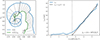 |
Fig. A.1. Left: Evolution of the torus angular-momentum vector L(t) (blue line) and the precession axis given by the torque, Laxis(t) = iτacc(t)/ωp (green line) in the simulation. The gray lines show their relative position at times spaced by constant intervals of Δt = 1.148 × 10³(GM/c3). Right: Precession angle relative to the precession axis Laxis as function of time, γrel(t) = arg[L(t)−iτ(t)/ωp]. Starting at t0 = 2.6 × 10³(GM/c3) the torus executes a nearly steady precession with frequency ωp = 5 × 10⁻⁴c3/(GM). |
All Figures
|
Fig. 1. Geometry of our model. The direction of the black-hole angular momentum (LBH) coincides with the z-direction of the Cartesian system used in the calculations. Due to misalignment with the black-hole spin, the angular momenta of the outer thin accretion disk (Ldisk) and inner hot torus (L) have nonzero projections onto the x-y plane. |
| In the text | |
|
Fig. 2. Precession of the angular momentum vector (L) of the inner torus when a steady accretion torque τf = τA is applied. This figure is projected into the plane perpendicular to the black-hole spin. In the absence of an accretion torque, the angular momentum vector executes free Lense-Thirring precession, LLT(t), around the direction of the black hole spin. When the torque is applied, the general solution consists of free Lense-Thirring precession about a new direction, shifted by a constant, |
| In the text | |
|
Fig. 3. Trajectory of the torus angular-momentum vector in the x-y plane when the accretion torque evolves exponentially from zero to τf = −1 for various cases. A torus that is initially precessing with an angular momentum L(0) = − 0.3i approaches the final state of precession about the new equilibrium point, iτf/ωp, slowly or rapidly for a low (ωh = 0.2ωp) or high (ωh = 2ωp) healing frequency, as in the left and middle panels, respectively. The right panel presents the same case as in the left panel (i.e., ωh = 0.2ωp), except that initially the torus has a zero angular momentum projection onto the x-y plane, i.e., L(0) = 0, highlighting that a change in accretion torque can induce precession in a torus. In all three examples, we set ωp = 1 and the phase evolution is represented by both the color and the decreasing thickness of the curve. |
| In the text | |
|
Fig. 4. Trajectory of the torus angular momentum vector in the x-y plane for an accretion torque rotating with frequency ω1 = 0.9ωp (left panel) and ω1 = 0.65ωp (right panel). In both cases, we use L(0) = 7i, τA = 1, and ωp = 1. The phase of the trajectory is represented by both the color and the decreasing thickness of the curve, with the starting point at t = 0, and a point later in time t marked by a circle and a triangle, respectively (for visualization purposes). The torus precesses around the black hole axis with a frequency of (ωp + ω1)/2. Additionally, the tilt angle between the black hole and torus oscillates with frequency (ωp − ω1). |
| In the text | |
|
Fig. 5. Comparison of our model with the simulation data of Bollimpalli et al. (2024). In the left panel, we show the magnitude of the accretion (dashed, fluctuating curve) and Lense-Thirring (smooth, solid curve) torques integrated over the torus region, i.e., 5–15 GM/c2. The difference between the two magnitudes (dotted, black curve) remains close to zero in the initial phase of the simulation, up to ∼25 000 GM/c3. The middle panel shows the x and y components of the net accretion torque on the torus (solid curves) and their respective fits using Eq. (20) (dashed curves). Finally, the right panel shows the x and y components of the total angular momentum of the torus (solid curves) and their respective fits using Eq. (21) (dashed curves). The vertical dashed black lines in all panels indicate the stop time of the original simulation. |
| In the text | |
|
Fig. A.1. Left: Evolution of the torus angular-momentum vector L(t) (blue line) and the precession axis given by the torque, Laxis(t) = iτacc(t)/ωp (green line) in the simulation. The gray lines show their relative position at times spaced by constant intervals of Δt = 1.148 × 10³(GM/c3). Right: Precession angle relative to the precession axis Laxis as function of time, γrel(t) = arg[L(t)−iτ(t)/ωp]. Starting at t0 = 2.6 × 10³(GM/c3) the torus executes a nearly steady precession with frequency ωp = 5 × 10⁻⁴c3/(GM). |
| In the text | |
Current usage metrics show cumulative count of Article Views (full-text article views including HTML views, PDF and ePub downloads, according to the available data) and Abstracts Views on Vision4Press platform.
Data correspond to usage on the plateform after 2015. The current usage metrics is available 48-96 hours after online publication and is updated daily on week days.
Initial download of the metrics may take a while.