| Issue |
A&A
Volume 707, March 2026
|
|
|---|---|---|
| Article Number | A207 | |
| Number of page(s) | 19 | |
| Section | Astrophysical processes | |
| DOI | https://doi.org/10.1051/0004-6361/202555753 | |
| Published online | 05 March 2026 | |
The effects of the spin and quadrupole moment of SgrA* on the orbits of S stars
1
LIRA, Observatoire de Paris, Université PSL, CNRS, Sorbonne Université, Université Paris Cité 5 Place Jules Janssen 92195 Meudon, France
2
Advanced Concepts Team, European Space Agency, TEC-SF, ES-TEC Keplerlaan 1 NL-2201 AZ Noordwijk, The Netherlands
★ Corresponding author: This email address is being protected from spambots. You need JavaScript enabled to view it.
Received:
30
May
2025
Accepted:
4
January
2026
Abstract
Context. Measuring the astrometric and spectroscopic data of stars orbiting the central black hole in our galaxy (Sgr A*) offers a promising way to detect relativistic effects. In principle, the “no-hair” theorem can be tested at the Galactic Center by monitoring the orbital precession of S stars caused by the angular momentum (spin) and quadrupole moment of Sgr A*. Closer-in stars, which tend to be more strongly affected by the black hole’s rotation, might be required for such studies. While such stars are currently too faint for GRAVITY, it would be possible to detect them with GRAVITY+.
Aims. We aim to analytically and numerically characterize orbital reorientations induced by spin-related effects of Sgr A* up to the second post-Newtonian (2PN) order.
Methods. To study the interaction between the orbital and spin orientations, we introduced observer-independent quantities that offer insight into the Kerr geometry. We also used the PN code OOGRE to simulate hypothetical stars orbiting closer to Sgr A*, where the spin and quadrupole effects are stronger. This enabled comparison with our analytical predictions.
Results. We exhibit three orbital-timescale precession rates that encode the in-plane pericenter shift and the out-of-plane redirection of the osculating ellipse. We provide the 2PN expressions of these precession rates and express the orbit-integrated associated angular shifts of the pericenter and of the ellipse axes. We relate these orbital-timescale precession rates to the secular-timescale precession of the orbital angular momentum around the black hole spin axis. We consider the theoretical insight provided in this article to be useful in constraining the spin effect of Sgr A* with GRAVITY+ observations.
Key words: black hole physics / gravitation / relativistic processes / instrumentation: interferometers / Galaxy: center
© The Authors 2026
 Open Access article, published by EDP Sciences, under the terms of the Creative Commons Attribution License (https://creativecommons.org/licenses/by/4.0), which permits unrestricted use, distribution, and reproduction in any medium, provided the original work is properly cited.
This article is published in open access under the Subscribe to Open model. This email address is being protected from spambots. You need JavaScript enabled to view it. to support open access publication.
1. Introduction
After years of monitoring S stars in the central parsec of the Milky Way, observational studies have demonstrated the presence of a supermassive compact object called Sgr A* at the center of the Galaxy (Eckart & Genzel 1996; Ghez et al. 1998, 2003, 2008; Schödel et al. 2002; Gillessen et al. 2009, 2017; GRAVITY Collaboration 2022), which is very likely a supermassive black hole (SMBH). According to the “no-hair” theorem, a black hole can be completely characterized by only three externally observable classical parameters: mass, angular momentum (hereafter, referred to as the spin), and electric charge. We assume that the BH charge can be neglected and, thus, we consider that the BH could be fully characterized by only its mass and spin and, furthermore, it can described within the framework of general relativity (GR) by the Kerr metric. This theorem implies that if we consider a higher moment of the gravity field, such as the mass quadrupole, it must be linked to the mass and spin, meaning that this theorem can be tested by independently measuring these three quantities and verifying the relation between them. Dozens of S star orbits are currently known (Gillessen et al. 2017), including the highly elliptical one of the star S2 with a 16-year period, reaching R ≈ 1400RS ≈ 120 AU from Sgr A* at its pericenter, where RS = 2GM•/c2, with G and M• being the gravitational constant and the black hole’s mass respectively. The mass of Sgr A* had already been measured from AO-assisted imaging and spectroscopy of S stars, but by combining the infrared light collected by the four Unit Telescopes of the Very Large Telescope (VLT) at Paranal, the interferometric instrument GRAVITY has provided a much more precise determination, M• = (4.2996 ± 0.0118)×106 M⊙ (GRAVITY Collaboration 2024). This increase in precision is a crucial step: it brings us to the level where future monitoring of S stars could, in principle, constrain the spin and quadrupole moment of the black hole (Will 2008; Angélil & Saha 2014), thereby enabling tests of the “no-hair” theorem.
As stated in Yu et al. (2016), understanding the spin direction of a supermassive black hole is also important because it can reveal clues about its growth history. For example, if the black hole spin is aligned with the young stellar disk in the Galactic Center, it could suggest that the black hole grew mainly from a gas disk that once matched the stellar disk. However, if the spin direction is very different from the stellar disk, it could mean that the black hole’s growth came from multiple chaotic accretion events, rather than one major episode. The different relativistic effects that can be observed in the vicinity of a strong gravitational field, such as the one surrounding Sgr A*, include:
-
Schwarzschild precession;
-
Shapiro time delay;
-
Relativistic redshifts (transverse Doppler shift in special relativity as well as the gravitational redshift appearing in GR);
-
Gravitational lensing effect;
-
Relativistic aberration.
In the case of a rotating black hole, we need to add the Kerr effects that arise from the rotation of the black hole to this list, namely:
-
Lense-Thirring (LT) effect, which results from the rotation of the body (e.g., a spinning black hole) distorts spacetime, causing nearby inertial frames to be “dragged” along with the rotation (also known as the frame-dragging effect). It impacts both the star orbit and photon trajectory and varies depending on the norm and the direction of the spin relative to the star’s orbit and affects both the astrometry and the spectroscopy;
-
Quadrupole moment effect, which is due to the oblateness of the black hole arising from its rotation. Similarly to the LT effect, this one also impacts both the star orbit and photon trajectory, varying depending on the norm and the direction of the spin relative to the star’s orbit, affecting both the astrometry and the spectroscopy.
In Sect. 3.1, we discuss the post-Newtonian (PN) expression of the Schwarzschild and spin-related accelerations. From a precession point of view, the Schwarzschild precession is the most dominant relativistic effect, leading to a pericenter advance. If the black hole is rotating, then the LT and the quadrupole moment effects end up generating both apsidal (in-plane) precession and nodal (out-of-plane) precession; as opposed to the Schwarzschild case, which only has an in-plane effect. This absence of out-of-plane precession in the Schwarzschild case is a direct consequence of the spherical symmetry of the Schwarzschild solution. The detection of the Schwarzschild precession was made possible with S2 and other stars (GRAVITY Collaboration 2020, 2024); however, the higher order Kerr effects prove to be more challenging, especially with respect to the quadrupole moment. By measuring the evolution of the orbital orientations of multiple closer-in stars (Will 2008), it is possible to constrain the value and orientation of the spin, along with the magnitude of the quadrupole moment. However, considering how quickly these higher order effects fall with distance from Sgr A*, we would likely need to work with stars that have shorter periods and/or higher eccentricities if we want to test the no-hair theorem in a relatively short timescale (Grould et al. 2017; Waisberg et al. 2018). Therefore, we considered putative stars multiple times closer to Sgr A* and, thus, much more affected by Kerr effects. Such stars might exist if they are too faint to have been already detected by GRAVITY. Furthermore, GRAVITY+ (the upgrade of GRAVITY and of the VLTI infrastructure) is now close to completion and will very soon have the potential to track stars on orbits closer to the black hole than S2, which have thus far been too faint to observe (GRAVITY Collaboration 2022). Therefore, it might become possible to not only constrain the spin parameters, but also the quadrupole moment. We note that there are different effects that have the most potential to interfere with the detection the LT or quadrupole moment effects, but that we did not consider in this work, include (Alush & Stone 2022): mass-precession (Merritt et al. 2010), star spin (Dixon 1970), vector resonant relaxation (Kocsis & Tremaine 2015; Merritt et al. 2010), and tidal disruption (Psaltis et al. 2013; Fabrycky & Tremaine 2007).
Astrometric and spectroscopic data both have the power to detect spin and quadrupole relativistic effects. If current spectroscopic data do not yet have the required precision to detect these effects at the present time, the perspective of the exquisite spectroscopic precision of ELT/MICADO ESO (2025) will most likely allow a very significant contribution of spectroscopy in the constraint of Sgr A*’s spin. However, in this article, we restricted ourselves to studying astrometric effects only. This choice is motivated by two reasons. First, GRAVITY+ already has the power to strongly constrain the spin of Sgr A* based on putative future-detected closer-in stars, without necessarily needing to wait for the first light of MICADO. Second, even in the ELT era, astrometry will still play a crucial role in stellar fittings aimed at constraining Sgr A*’s spin. Indeed, the impact of spectroscopy for spin detection is particularly striking when data are available close to the pericenter passage. In this situation, spectroscopy might overcome the power of astrometry. On the contrary, astrometry is able to significantly constrain the spin effect along the full trajectory. As a consequence, astrometry and spectroscopy appear as two very complementary probes, with astrometry being particularly crucial if spectroscopic data closest to pericenter cannot be secured.
This paper is organized as follows. We present in Sect. 2 an overview of the framework used in our study. The derivation of the relativistic orbital precessions in the PN approximation is laid out in Sect. 3. In Sect. 4, we use the OOGRE code to study how the spin and quadrupole moment affect the evolution of orbits. Finally, we summarize and discussing the applicability of our results to upcoming observations in Sect. 5.
2. Reference frames
We begin this work by properly laying out the framework and present the four reference frames1 that are needed. Following the convention of Poisson & Will (2014) and Merritt (2013), we introduced a so-called fundamental frame (X, Y, Z) and used it as an arbitrary reference for describing the problem. Considering that we eventually want to model the observable in the sky plane, it is natural to choose the observer’s frame as the fundamental one. For this purpose (as illustrated in Fig. 1), we took Z as pointing towards the observer and (X, Y) = (δ, α) = (Dec, RA) corresponding to the observer’s screen with α or RA and δ or Dec referring to the right ascension and declination, respectively. In other words, we defined the fundamental plane as the sky plane and center it on the apparent position of Sgr A*. This choice has a crucial impact on the definition of orbital parameters considering that the angular parameters are defined with respect to the fundamental frame. In the literature, we can find different definitions of the observer’s frame and fundamental frame. This leads to different results that cause apparent contradictions, as noted in the following sections and appendices.
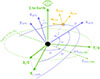 |
Fig. 1. Orbit frame (xorb, yorb, zorb) and orbital elements are represented in purple, while the fundamental frame (X, Y, Z) is in green. The pericenter, represented by the point 𝒫, is also added. Finally, ℒorb//sky denotes the line of nodes of the orbit frame and sky plane. We also represent the Gaussian frame of the star (norb, morb, zorb), the projection of the X axis on the orbit plane denoted by X//orb and the angle, ϖ, introduced in Sect. 4. Here, we illustrate the fundamental frame when it matches that of a distant observer (see Sect. 2). Also, it is useful to note the the azimuthal angle is φ = ω + f. |
The problem we study in this work refers to a star in a bound orbit around a rotating black hole. Thus, we need to describe two vectors in the fundamental frame: the angular momentum of the orbit and the angular momentum of the black hole, which naturally define two other frames, namely, that of the orbit and that of the black hole.
The orbit frame (xorb, yorb, zorb) is illustrated by Fig. 1. The axis zorb is along the angular momentum of the orbit, such that the plane (xorb, yorb) matches the instantaneous plane2 of the orbit. Also, xorb always points to the instantaneous pericenter of the orbit (we recall that the pericenter of a relativistic orbit is not fixed; see the notion of osculating orbital parameters noted in Appendix A). Further details on the line of nodes ℒorb//sky and the ascending node of the orbit 𝒜𝒩orb//sky are provided in Appendix B. The orbital parameters that are included in Fig. 1 are discussed further in Appendix A.1. For the time being, it is useful to note that the orientation of an orbit is characterized by three angles: the two angles ι and Ω define the orientation of the orbital plane relative to the fundamental frame, while the third angle ω defines the position of the pericenter inside the orbital plane. In addition, it is useful to introduce the Gaussian frame3 (norb, morb, zorb), which follows the movement of the star as illustrated in Fig. 1; norb is the radial vector and morb completes the orthonormal basis.
The black hole frame (xbh, ybh, zbh), labeled in cartesian coordinates, is illustrated in Fig. 2. It is defined such that the angular momentum (or spin vector) of the black hole is along zbh. The orientation of xbh and ybh is arbitrary. We introduce the angles (θ, β) that allow to orient zbh in the orbit frame as defined in Fig. 2:
-
θ ∈ [0; π] is the rotation angle from zorb to zbh;
-
β ∈ [0; 2π] is the rotation angle about zorb, from ℒorb//sky to zbh//orb.
We also introduce an alternative definition of angles (i′,Ω′) in Appendix B that are useful for performing multi-star fits. These angles are not considered further in this article.
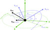 |
Fig. 2. Angles (θ, β) in purple characterize the orientation of the spin vector, zbh, relative to the orbit frame. We also added the angle ψ ≡ β − ω, so that (θ, ψ) are the spherical coordinates of the spin axis in the orbit frame. The projection of zbh on the orbit plane is denoted by zbh//orb. |
3. Post-Newtonian expressions of the secular shifts
3.1. Post-Newtonian acceleration
Here, we focus on the PN formalism, which allows us to separate the LT effect from the quadrupole moment effect. For the PN formalism, we used harmonic coordinates, which are commonly used in works on PN (Poisson & Will 2014). In the PN approximation, the equation of motion of a star of negligible mass, mstar, compared to the mass of the black hole, M•, (Poisson & Will 2014) is expressed as
 (1)
(1)
where m = M• + mstar ≈ M•. This approximation is referred to as ❶ and can be justified by the fact that the small PN parameter ϵ = GM/(c2p) is at least one or two orders of magnitude greater than η = mstar/M• ∼ 10−6 − 10−5 for any hypothetical star relevant for our study (mstar ∼ 1 − 10 M⊙ and with p ≤ pS2). The separation vector from the black hole to the star is denoted by r, while norb = r/r is expressed as
 (2)
(2)
where p = asma(1 − e2) is the semi-latus rectum. Sometimes, p and e are alternatively defined as constants even in GR using the pericenter and apocenter radii r− and r+ by: p = r−(1 + e) = r+(1 − e). However, this definition will yield a different definition of the pericenter advance compared to p = asma(1 − e2), (see Tucker & Will 2019). A dot in (1) denotes derivation with respect to the harmonic-coordinate time t and the PN acceleration aPN accounts for deviations from Keplerian motion due to GR. Thanks to the use of the osculating orbital elements method, we are able to use the Newtonian relation of Eq. (2) at each date, while keeping in mind that the involved parameters are time-varying as well as the fact that we are using the weak-field and small-velocity approximations when working with the PN formalism.
If we want to understand, at leading order, how the Schwarzschild precession and the spin-related effects impact the orbit of S stars, it is sufficient to look at the dominant order of the analytical expressions of the secular shifts of orbital elements (Will 2008). In practice, however, since the PN formalism appears to be the most suitable for the process of fitting the data of S stars4, we have to choose one specific PN order for all effects to be consistent in the fitting process. As discussed in this section, the dominant order of the LT and quadrupole moment effects are at the 1.5PN (corresponding to (v/c)3) and 2PN orders (corresponding to (v/c)4), respectively. Therefore, we need to first obtain the analytical expressions up to the 2PN order.
Considering the second-order PN approximation (2PN) corresponding to (v/c)4, the PN acceleration can be decomposed into three parts:
 (3)
(3)
with  ,
,  ,
,  corresponding to the 2PN acceleration of the star due to the Schwarzschild precession, the spin and the quadrupole moment, respectively. This approximation is referred to as ❷. The kPN notation indicates the PN order up to which the various effects enter the equation of motion. For instance
  contains both the 1PN and 2PN Schwarzschild contributions. By considering approximation ❶ and by defining the small PN parameter as
 (4)
(4)
the accelerations can be expressed in terms of ϵ as (Merritt 2013; Will 2008; Blanchet & Iyer 2003):
 (5)
(5)
![Mathematical equation: $$ \begin{aligned}&\mathbf a _{\rm LT}^{\mathrm{1.5PN} } = -2\epsilon ^{3/2} \sqrt{\frac{G m}{p^3}}(1+e\cos f)^3\chi \nonumber \\&\quad \quad \times \left[2\boldsymbol{v} \times \mathbf z _{\mathrm{bh} }- 3\left(\mathbf n _{\mathrm{orb} }\cdot \boldsymbol{v}\right)\mathbf n _{\mathrm{orb} } \times \mathbf z _{\mathrm{bh} }-3\mathbf n _{\mathrm{orb} } \left(\mathbf n _{\mathrm{orb} } \times \boldsymbol{v}\right)\cdot \mathbf z _{\mathrm{bh} }\right], \end{aligned} $$](/articles/aa/full_html/2026/03/aa55753-25/aa55753-25-eq10.gif) (6)
(6)
 (7)
(7)
with v2 = vr2 + vt2 and χ being the spin parameter. The latter is positive and has a maximal value of 1 (for a Kerr black hole). The dimensionless spin vector, χ = χzbh, is linked to the angular momentum, J = Jzbh, of a black hole of mass, M•, via
 (8)
(8)
As for the quadrupole moment parameter Q, we note that it enters Eq. (7) via
 (9)
(9)
where the fact that Q depends only on M• and χ is a consequence of the no-hair theorem (Poisson 1998; Krishnendu et al. 2019).
We note that the Schwarzschild acceleration is composed of two terms, namely, orders of 1PN and 2PN. The LT and quadrupole moment accelerations are composed of only one term of an order of 1.5PN and 2PN, respectively. The leading order of the various effects is thus 1PN, 1.5PN, 2PN, for the Schwarzschild, LT, and quadrupole moment effects, respectively. We need to consider the subleading order only for the Schwarzschild term. The LT and quadrupole moment subleading terms appear at order above 2PN. In this paper, we consider only the Kerr spacetime, and, thus, we plugged the expression of Q given by Eq. (9) into our equations. However, if we want to test the no-hair theorem, we should not assume Eq. (9) when generating the expression of the secular shifts5, since Q would need to be measured independently of χ.
3.2. Lagrange planetary equations
We can use the orbital perturbation theory (Merritt 2013; Will 2008) to express the derivative of each time-varying, osculating orbital parameter with respect to time, as a function of the various ℛ, 𝒮, and 𝒲 terms, the perturbative accelerations expressed in the Gaussian frame, introduced in Appendix C (also see Poisson & Will 2014, for details). They are called the Lagrange planetary equations6 and are expressed as
 (10)
(10)
![Mathematical equation: $$ \begin{aligned}&\frac{\mathrm{d}e}{\mathrm{d}t} = \sqrt{\frac{p}{Gm}} \left[\sin f \mathcal{R} + \frac{2\cos f+e(1+\cos ^{2}f)}{1+e\cos f} \mathcal{S} \right]; \end{aligned} $$](/articles/aa/full_html/2026/03/aa55753-25/aa55753-25-eq15.gif) (11)
(11)
 (12)
(12)
 (13)
(13)
![Mathematical equation: $$ \begin{aligned}&\frac{\mathrm{d}\omega }{\mathrm{d}t} = \frac{1}{e}\sqrt{\frac{p}{Gm}} \left[-\cos f \mathcal{R} + \frac{2+e\cos f}{1+e\cos f} \sin f \mathcal{S} \right.\nonumber \\&\;\;\qquad \qquad \qquad \left. -e\cot \iota \frac{\sin (\omega +f)}{1+e\cos f} \mathcal{W} \right]. \end{aligned} $$](/articles/aa/full_html/2026/03/aa55753-25/aa55753-25-eq18.gif) (14)
(14)
No approximations are done to obtain Eqs. (10)–(14) from Eqs. (1).
As stated earlier, in the context of a small perturbing force, it is possible to get a good estimation of the orbital dynamics by only looking at the dominant contribution of each effect. To do so, we solve the equations within the framework of perturbation theory and find that, to express the leading order of such an effect for a given orbital parameter, it is appropriate to take the 0PN terms of all other orbital parameters in the right-hand side of Eqs. (10)–(15), before integrating these equations over t. Even more convenient would be to use f as an independent variable instead of t, considering it has the same fixed integration interval over one period for any star. It evolves as (see Poisson & Will 2014, for details):
![Mathematical equation: $$ \begin{aligned} \frac{\mathrm{d}f}{\mathrm{d}t}&= \left(\frac{\mathrm{d}f}{\mathrm{d}t}\right)_{\mathrm{Kepler} }-\left(\frac{\mathrm{d}\omega }{\mathrm{d}t} +\cos \iota \frac{\mathrm{d}\Omega }{\mathrm{d}t}\right)\nonumber \\&= \sqrt{\frac{Gm}{p^3}}(1+e\cos f)^{2}\nonumber \\&\quad + \frac{1}{e} \sqrt{\frac{p}{Gm}}\left[\cos f \mathcal{R} -\frac{2+e\cos f}{1+e\cos f}\sin f \mathcal{S} \right], \end{aligned} $$](/articles/aa/full_html/2026/03/aa55753-25/aa55753-25-eq19.gif) (15)
(15)
where we recall the fact that f is the angle between the varying pericenter and the position vector of the star r (see Fig. 1). We can make use of the fact that the term  is Keplerian (0PN) and that the non-Keplerian terms on the right-hand side of Eq. (15) start at 1PN, 1.5PN, and 2PN orders for the Schwarzschild, LT, and quadrupole moment effects, respectively. This means that we are allowed to express the temporal variation as
![Mathematical equation: $$ \begin{aligned} \frac{\mathrm{d}t}{\mathrm{d}f} = \sqrt{\frac{p^3}{Gm}}\frac{1}{(1+e\cos f)^{2}}\left[1+\mathcal{O} (\epsilon )\right], \end{aligned} $$](/articles/aa/full_html/2026/03/aa55753-25/aa55753-25-eq21.gif) (16)
(16)
before multiplying Eqs. (10)–(14) by the zeroth-order term of Eq. (16) to get the dominant order derivative of each orbital parameter with respect to the true anomaly, f.
3.3. Analytical integration of the planetary equations
Now that we have the expression of the planetary equation as a function of f, we integrated them with f from f0 to f0 + 2π7 to find the dominant terms of the secular evolution of the orbital parameters. By considering the Keplerian dominant constant term of p, e, ω, and β on the right-hand side of Langrange planetary equations, we find that p and e (and, consequently, asma and P) do not show any secular variations after one orbit at the dominant orders. As for the other parameters, we find that the precessions per orbit of a star’s argument of periapsis, Δω, along with the longitude of the ascending node, ΔΩ, and inclination, Δι verify8, the following:
 (17)
(17)
 (18)
(18)
 (19)
(19)
 (20)
(20)
 (21)
(21)
 (22)
(22)
 (23)
(23)
 (24)
(24)
 (25)
(25)
We note that Will (2008) adopted the same definition of fundamental frame as we have in our work, which is why we agree on the variation of the angular orbital parameters. However, our Eqs. (21) and (22) should not be compared with Eqs. (3.23a) of Will & Maitra (2017) and (5) of Tucker & Will (2019) since we have made a different choice of fundamental frame from theirs, leading to different definitions of ι and Ω among other parameters.
These secular trends are valid at 2PN order for the LT and quadrupole moment shifts, for which subleading contributions appear at orders higher than 2PN. However, for the Schwarzschild terms, we need to compute the subleading 2PN contribution, in addition to the leading 1PN contribution provided above.
To do so, the two-timescale method detailed in Appendix D can be used to account for the periodic evolution of the orbital parameters. This method requires introducing a small parameter similar to ϵ, but nonvarying, which we label with the orbit-averaged quantity,  . Accordingly, the 2PN pericenter advance takes the following form:
 (26)
(26)
 (27)
(27)
 (28)
(28)
which are more precise analytical expressions than those given in Alush & Stone (2022). When expressing the pericenter advance to 2PN accuracy, it is therefore essential to use the orbit-averaged parameters  and
and  , rather than their osculating or varying counterparts. Using the latter in the 1PN term would already introduce discrepancies at 2PN order. At leading order, however, we can safely identify
  , so this subtlety has no impact on Eqs. (17)–(25). A more detailed justification of this choice is provided in Appendix D.2. We note that if ι = 0, ℒorb//sky cannot be defined as it is degenerate, then ω and Ω, and thus Eqs. (18), (19), (24), and (25) cannot be defined either. This issue can be addressed by introducing new variables, as explained in Sect. 4.
3.4. Numerical integration of the planetary equations
To numerically integrate the planetary equations to simulate orbits, we used our Python-based code called Osculating Orbits in General Relativistic Environments (OOGRE), which was originally developed by Heißel et al. (2022). It is a perturbed Kepler-orbit model code that is based on the formalism presented in Sect. 3.1 and optimized for stars in the Galactic Center.
The goal of Sect. 4 is to investigate the impact of Kerr effects on the geometry of the orbit; the interest primarily lies in the dynamical interaction between the black hole and one star. Therefore, we do not consider the effect of mass-precession and vector resonant relaxation, while also neglecting the tidal disruption and effect of the star’s spin. Moreover, as the goal is not to simulate observations here, we turned off the following effects, as we find they would interfere with this goal:
-
the Shapiro time delay;
-
the Rømer effect;
-
the gravitational lensing9.
Also, the relativistic aberration is not implemented in OOGRE and is not needed for the purposes of this discussion either. However, we extended this code, which initially only considers  , to the Kerr metric by adding the spin and quadrupole moment contributions,
  and
and  , to simulate these effects. We also pushed the Schwarzschild precession to the 2PN order with
  for consistency.
We chose a set of initial conditions as in Heißel et al. (2022), and fix the osculating time as tosc = tperi − Posc/2, an approximate10 value of the apocenter, granting the code more stability. The code integrates Eqs. (10)–(14) at the core of OOGRE while only using the approximations ❶ and ❷.
4. Spin impact on the orientation of the orbit
First, we want to understand analytically the effect of spin on the evolution of the orientation of the orbit. This leads us to introduce several precession movements, either instantaneous or secular. The secular evolution is well known (see e.g., Kocsis & Tremaine 2011) and consists of a precession movement of zorb about zbh. Instantaneous evolution is both less known and more useful in the perspective of orbital fits. Therefore, we focus on the latter in the discussion below. Second, we want to illustrate this analytical understanding by performing simulations for a hypothetical closer-in star, which we call “S2/10”.
4.1. Instantaneous orientation change
4.1.1. Orbital frame orientation change
We start by characterizing the evolution of the orientation of the orbit by expressing the temporal evolution of the orbit frame. Using the Lagrange planetary equations, it is possible to reexpress the temporal variations of these vectors as functions of the temporal variations of the orbital elements. We get (see Will et al. 2023):
 (29)
(29)
 (30)
(30)
 (31)
(31)
where s𝒲 is the sign of 𝒲 and
 (32)
(32)
 (33)
(33)
 (34)
(34)
We can add the last lines of Eqs. (29)–(31) to reveal the precession aspect of the equations and their different components.
Thus, we obtain
 (35)
(35)
encoding the change of direction of the major and minor axes in the orbit plane;
 (36)
(36)
encoding the change of the major axis orthogonal to the orbit plane, or equivalently the change of the orbital angular momentum direction along the major axis;
 (37)
(37)
encoding the change of the minor-axis direction orthogonal to the orbit plane, or equivalently the change of the orbital angular momentum along the minor axis. We note that  , as it should for unit vectors. Therefore, we can decompose the overall precession into two components: the precession of the argument of periapsis within the changing orbital plane, with associated characteristic frequency
  , hereafter referred to as “in-plane11 precession”; and the precessions of the orbit plane, with characteristic associated frequencies,
  and
and  , hereafter referred to as “out-of-plane precession”.
These scalar quantities are also presented12 in Will et al. (2023), and are independent from the observer’s location, which is obvious from their definition: they depend only on (xorb, yorb, zorb), which depends only on the orbit. As such, ϖ, Θ and Ξ appear to be very useful for expressing observer-independent statements on the variation of the pericenter and angular momentum directions.
4.1.2. Secular orientation change
We introduce the secular shifts Δϖ, ΔΘ, and ΔΞ, as the integration over an orbit of the temporal variations of ϖ, Θ, and Ξ. The secular in-plane shift of the pericenter can be expressed at 2PN order as
 (38)
(38)
 (39)
(39)
 (40)
(40)
We note that Eqs. (39) and (40) will still be valid if ι = 0, as opposed to Eqs. (18), (19), (24), and (25). Using ϖ allows us to quantify the precession inside the orbital plane without using the notion of ℒorb//sky which is degenerate in the case of a face-on13 orbit. From Eqs. (39) and (40) we see that the LT and quadrupole moment in-plane precession depend on the polar angle, θ, but not on the azimuthal angle, ψ, of the spin vector spherical coordinates defined in Fig. 2. We see that the in-plane precession of the LT effect is maximal for orbits in the equatorial plane of the black hole, namely, for θ = 0 (mod π), and it vanishes for polar14 orbits, namely, for θ = π/2 (mod π). However, the quadrupole moment in-plane precession is maximized for both equatorial and polar orbits and it vanishes for  .
.
The secular out-of-plane shift of the major axis can be expressed at 2PN order from Eq. (33) as
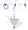 |
Fig. 3. Figure 3a shows the evolution of the orbit orientation on an orbital period P timescale. Three precessions are experienced: an in-plane precession (left panel) with contributions at 1PN, 1.5PN, and 2PN; and two out-of-plane precessions, namely, one around the minor axis (middle panel) and another around the major axis (right panel) with contributions at 1.5PN and 2PN. Figure 3b shows the evolution of the orbit orientation on a secular timescale Pcone ≫ P (see Eq. (E.1)). The orbital angular momentum experiences a precession around the black hole spin axis. |
 (41)
(41)
to characterize the out-of-plane component of the pericenter precession. When using the secular shifts of the orbital parameters derived in Sect. 3.3 in Eq. (41), we obtain the following expressions:
 (42)
(42)
 (43)
(43)
corresponding to the out-of-plane movement of the major axis precession (also referred to as out-of-plane apocenter shift) due to the LT and quadrupole moment effects, as illustrated in Fig. 3. The Schwarzschild precession does not contribute to the out-of-plane shifts at any PN order.
Finally, the secular out-of-plane shift of the minor axis can be expressed at 2PN order from Eq. (34) as
 (44)
(44)
We obtain the following expressions:
 (45)
(45)
 (46)
(46)
The expressions of ΔΘ and ΔΞ above show that these quantities depend on both θ and ψ. If we take ψ = π/2 (mod π), namely, when the projection of the spin axis of the black hole on the orbit is along the minor axis, then ΔΘ would be maximized, while ΔΞ would be null (i.e., the major axis precesses in a plane orthogonal to the minor axis). Conversely, with ψ = 0 (mod π), namely, when the projection of the spin axis on the orbit is along the major axis, ΔΘ would be null, while ΔΞ would be maximized (i.e., the minor axis precesses in a plane orthogonal to the major axis). We note that due to the in-plane precession, this can be true only instantaneously.
The LT effect generates a maximal out-of-plane precession for polar orbits and a vanishing one for equatorial orbits. We also see that the configuration that allows for the most apocenter displacement due to the LT effect (the maximum of  ) would be an equatorial orbit.
As for the quadrupole moment effect, it does not induce any out-of-plane precessions for polar orbits. In addition, we observe that the out-of-plane precession is maximized for θ = π/4 (mod π). This behavior is similar to the Newtonian case of a particle orbiting an oblate mass; if the particle is mid-inclined with respect to the equatorial plane of the central mass15, the particle would experience the highest level of asymmetries along the orbit leading to the highest out-of-plane shifts among all possible relative orientations (Boain 2004). In terms of overall apocenter angular shift, we also see that the configuration that maximizes  would be an equatorial orbit.
Even though ω and β are observer-dependent, ψ = β − ω, the angle between zbh//orb and xorb, rotating around zorb in Fig. 3, is observer-independent. Therefore, ΔΘ and ΔΞ are observer-independent as well.
4.2. Secular shifts for S2 and “S2/10”
Here, we consider the star S2, as well as a hypothetical star that can potentially be detected with GRAVITY+ and that we call “S2/10”. It is a star with an orbit identical to that of S2 but with a semimajor axis 10 times smaller. In Table 1, we compare the various maximal secular shifts of the star S2. To compare these shifts using a single set of orbital parameters, we used osculating orbital elements at apocenter.
Comparing the various maximal secular shifts of the star S2.
When computing the secular shifts for “S2/10”, we can see that
with X denoting either in-plane (ϖ) or out-of-plane (Θ, Ξ) precession components. This scaling between the Schwarzschild precession and the LT and the quadrupole moment effects arises from their respective radial dependencies, which are encapsulated by the parameter ϵ. While the intrinsic relativistic precessions increase steeply for smaller semimajor axes (as shown by the scaling relations above), the corresponding astrometric signatures on sky do not necessarily become easier to detect. Indeed, in astrometry, we measure projected positions rather than orbital angles, and the apparent size of the orbit scales linearly with asma/R0. For such a star as “S2/10”, the orbit would appear ten times smaller on sky than that of S2, partly compensating for the intrinsic amplification of the relativistic effects. As a result, the gain in the astrometric measurability is only increased by a factor  and 10 for the LT effect and quadrupole term, while the Schwarzschild precession would remain essentially unchanged in relative detectability. Nevertheless, having smaller periods allows us to observe more pericenter and apocenter passages, thereby accumulating more secular shifts in a given amount of time. For instance, the period of the star S2 (≈16 yr) corresponds to 103/2 ≈ 32 orbits of the star “S2/10”. Therefore, when working with “S2/10”, instead of S2 over one period of S2, the astrometric measurability of the Schwarzschild precession is increased by a factor ≈103/2 ≈ 32, the LT precessions by a factor
  , and the quadrupole moment shifts by a factor 103/2 × 10 ≈ 320. These scaling behaviors emphasize the scientific value of observing closer-in stars, providing a powerful means to probe both the spin and higher order mass moments of Sgr A*.
4.3. Time-averaged orientation change
After describing the instantaneous orientation change of the orbital frame, we go on to discuss its secular evolution over long timescales (as compared to the orbital period). We know from Eqs. (12), (13) and (31), along with the corresponding expression of the perturbative acceleration given in Eq. (C.8), that the LT effect acts on the orbital angular momentum such that
![Mathematical equation: $$ \begin{aligned} \frac{\mathrm{d} \mathbf{z }_{\mathrm{orb} }}{\mathrm{d} t}\bigg |_{\rm LT}\!\!\!\! = -2\frac{G^{2}m^{2}}{c^3r^3}\chi \left[\frac{e\sin f}{1+e\cos f}(\mathbf{z }_{\mathrm{bh} } \cdot \mathbf{m }_{\mathrm{orb} }) + 2(\mathbf{z }_{\mathrm{bh} } \cdot \mathbf{n }_{\mathrm{orb} })\right] \mathbf{m }_{\mathrm{orb} }. \end{aligned} $$](/articles/aa/full_html/2026/03/aa55753-25/aa55753-25-eq72.gif) (47)
(47)
From this we obtain16:
 (48)
(48)
where17:
 (49)
(49)
and  is the Newtonian mean motion. Moreover, we have the expression (see Fig. 2):
 (50)
(50)
which we can then insert into Eq. (48). Next, by identifying to the time average of Eq. (31), we can define:
 (51)
(51)
 (52)
(52)
and thus get
 (53)
(53)
 (54)
(54)
This shows that  and
and  are the time-average of
  and
and  and that
  and
and  . In other words, we end up with the same results given by the instantaneous formalism used in Sect. 4.1, which links the two aspects of instantaneous and averaged precession shifts.
If we do the same exercise for the quadrupole moment using Eqs. (31) and (C.9), we get
 (55)
(55)
where
 (56)
(56)
Once again, we see that  and
and  as with the the LT effect discussed above.
We see from Eqs. (48) and (55) that zorb has an average precession around zbh, meaning that the angle θ between zorb and zbh has no secular evolution. In other words, the secular out-of-plane precession is done at fixed18θ, of zorb about zbh (as illustrated in Fig. 3), and Eqs. (49) and (56) are the frequencies at which the out-of-plane precession spans the cone of angle θ represented in Fig. 3, due to the LT (at the 1.5PN order) and quadrupole moment (at the 2PN order) effects, respectively. We also see that the direction of secular rotation of zorb due to the LT effect is the same as that of the spin. The direction of secular rotation of zorb due to the quadrupole moment effect depends on the sign of −zbh ⋅ zorb = −cos θ, as shown by Eq. (55); in the case of θ > π/2 (a retrograde orbit relative to the black hole), the direction of rotation is the same as that of the spin, for example. However, the opposite is true in the case of prograde orbits relative to the black hole.
In conclusion, we stress that both the in-plane and out-of-plane precessions can be considered differently on two timescales: time-averaged (on the cone defined by Eqs. (48) and (55) for the out-of-plane precession) and instantaneously, which corresponds to a rotation of the axes around each other, given by Eqs. (29) and (31). We note that it can also deviate from the cone defined by Eqs. (48) and (55) for the out-of-plane precession.
4.4. Numerical illustration
We illustrate the instantaneous variations in the orientation of the orbital frame using numerical integrations of the PN Lagrange planetary equations (see Sect. 3.2). These simulations were tailored to maximize the impact of each relativistic effect (see the analysis of Sect. 4.1.2). To do so, we aligned zbh on each axis of the orbit frame, zbh//zorb (maximizing the in-plane precession of all effects), zbh//xorb and zbh//yorb (maximizing the out-of-plane precession of the LT effect); these three configurations are referred to as “equatorial orbit”, “polar orbit with polar major axis”, and “polar orbit with equatorial major axis”, respectively. Finally, we refer to Appendix E for a discussion of the study of “mid-inclined orbits”, which maximize the out-of-plane precession of the quadrupole moment, where  . This provides an intuitive approach to the way the spin of the black hole can impact the orbit, independently of the observer.
The simulated star is taken to have orbital parameters identical to “S2/10” in terms of the semimajor axis and eccentricity. We performed a Euclidean projection of the orbit onto a plane, noting that this was for illustrative purposes only and does not aim at reproducing observables. Effects such as the Rømer delay, gravitational redshift or lensing were deliberately omitted, as they fall outside the scope of this analysis. In the following subsections, we show that the simulated variations in these configurations reproduce the expected PN trends, both in direction and in structure. We defined a prograde and retrograde orbit relative to the black hole, with angular momentum along  and
and  , as orbits verifying
  and
and  , respectively.
4.4.1. In-plane precession: Focusing on equatorial orbits
In this subsection, we examine the impact of the in-plane precession due to Kerr effects, independently of the projection on the screen of a distant observer. For this purpose, we simulated orbits that are in the equatorial plane of the black hole, thereby maximizing the in-plane precession and eliminating the out-of-plane ones19.
We considered two orbits in the equatorial plane of the black hole: one prograde (θ = 0) with  and the other retrograde (θ = π) with
  , making ψ degenerate. For understanding the in-plane precession, in Figs. 4 and 5, we offer a Euclidean projection of these orbits onto a face-on plane.
 |
Fig. 4. Prograde orbits in the equatorial plane of the black hole with a face-on view. Figure 4a displays a schematic illustration of the osculating Keplerian orbit (see Sect. 4.4.1) with the apocenter represented by the letter 𝒜. In Fig. 4b we show an orbit of the hypothetical star “S2/10” simulated in 2PN using OOGRE: the “✷” denotes the apocenters (the first apocenter in black corresponds to the osculating time, which is also the initial date, and is in common for the three orbits). We simulate one orbit for the Schwarzschild precession (“Sch” in orange), one orbit for both the Schwarzschild and LT precessions (“LT” in green), and one orbit for the Schwarzschild, spin and quadrupole moment precessions (“Q” in thin purple). We see that the LT and quadrupole moment effects shift the apocenter clockwise and counterclockwise, respectively, as seen by this face-on observer. All numbers are expressed in mas except otherwise noted. |
Let us start with the well-known Schwarzschild precession. We know that ω is measured in the same direction as the movement of the star in its orbit. When looking at the analytical expressions, we see that Eq. (38) is independent from θ, it leads to the same positive Δϖsch for prograde and retrograde orbits, regardless of the orientation of the black hole with respect to the orbit. This means that the prograde and retrograde apocenter displacements will go in opposite ways. We see in Figs. 4b and 5b that the Schwarzschild precession shifts the apocenters of the prograde and retrograde orbits counterclockwise and clockwise, respectively. In simpler words, the simulations agree with Eq. (38) in terms of orientation on the projection plane.
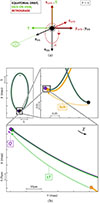 |
Fig. 5. Same as Fig. 4, but for retrograde orbits. We see that both the LT and quadrupole moment effects shift the apocenter clockwise as seen by this face-on observer. |
Now, let us examine the LT effect. Figure 4b indicates an apocenter shift opposite to the direction of the spin and the same is observed in Fig. 5b. Indeed, when looking at Eq. (39), we see that for the prograde orbit,  and
and  , meaning that both the prograde and retrograde apocenters will be shifted clockwise (i.e., opposite to the direction of the spin).
Finally, we see from Figs. 4b and 5b that, similarly to the Schwarzschild precession, the quadrupole moment shifts the apocenters in the same direction as the movement of the star in its orbit. Indeed, when looking at Eq. (40), we see that the sign of ΔϖQ depends only on the value of cos2θ meaning that ΔϖQpro = ΔϖQret > 0.
Finally, it is important to remember that all these effects do not share the same dominant PN order and, therefore, they do not act on the same scale. This is evident in Figs. 4b and 5b, where the Schwarzschild precession dominates the LT effect, which, in turn, dominates the quadrupole moment effect. Also, it is interesting to note that the total secular shift of orbits in the equatorial plane of a rotating black hole will differ in absolute value in the prograde and retrograde configurations; in the first case, the LT and quadrupole moment effects cancel each other out, whereas in the second case, they push the apocenter in the same direction.
If we summarize all the above, we get the following statements illustrated in Fig. 6:
-
The Schwarzschild precession pushes the apocenter in the same direction as the movement of the star in its orbit.
-
The secular shift due to the LT effect pushes the apocenter of an equatorial orbit in the direction opposite to the black hole’s rotation.
-
The secular shift due to the quadrupole moment pushes the apocenter of an equatorial orbit in the same direction as the movement of the star in its orbit.
-
The analytical total Kerr secular shift of equatorial orbits verifies
 .
.
4.4.2. Lense-Thirring out-of-plane precession
In this section, we want to illustrate the configurations that maximize the dominant spin-induced effect brought on by the LT precession. As suggested in Sect. 4.1.2, to better understand the out-of-plane precession of the LT and quadrupole moment effects, it is useful to split it into two subtypes, precession around the major axis of the orbit and precession around the minor axis, encoded by Eqs. (33) and (34), respectively. Therefore, we focus on two types of polar orbits, for which the out-of-plane component of this effect is strongest (see Sect. 4.1):
-
Polar orbit with polar major axis20: zbh//xorb i.e., (θ, ψ) = (π/2, 0);
-
Polar orbit with equatorial major axis: zbh//yorb i.e., (θ, ψ) = (π/2, π/2).
To visualize the out-of-plane components independently of the projection effects, we performed an edge-on Euclidean projection, considering that the osculating orbit is a vertical line with the apocenter at the bottom of the projection plane (see Figs. 7a and 8a).
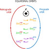 |
Fig. 6. Schematic illustration of the secular precessions for a prograde and a retrograde equatorial orbit. We note that Schwarzschild precession and quadrupole moment effect push the apocenter in the direction of stellar motion and the LT precession pushes against the spin. |
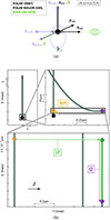 |
Fig. 7. Same as Fig. 4, but with orbits in a polar plane and having a major axis on the spin axis of the black hole (see Sect. 4.4.2). We see that the LT effect shifts the minor axis in the same direction as the the spin of the black hole, gradually shifting the orbit plane from edge-on towards face-on. The quadrupole moment effect shifts the apocenter clockwise as seen on face-on projection of Fig. 4a. |
We start with the first subtype, illustrated in Fig. 7, where the orbit lies in the polar plane of the BH and verifies zbh//xorb. As opposed to the equatorial orbits of Sect. 4.4.1, here the notion of prograde and retrograde orbits is more delicate. Polar orbits cannot be categorized as prograde or retrograde relative to the black hole and, furthermore, an orbit with an edge-on view cannot be categorized as prograde or retrograde relative to the observer. Therefore, we instead considered an orbit where the star is moving towards the observer at the apocenter (as illustrated in Fig. 7a).
We see from Sect. 4.1.2 that when assuming (θ, ψ) = (π/2, 0), the LT effect maximally contributes to the out-of-plane precession, while it does not contribute to the in-plane one; interestingly enough, the quadrupole moment has the opposite tendency. We recall that having ΔϖLT = 0, ΔΘLT = 0 and ΔΞLT ≠ 0 means that, instantaneously, the apocenter will not experience any secular precession attributed to the LT effect. However, as soon as the apocenter is shifted out of the spin axis due to other effects, the LT effect will also start contributing to the apocenter displacement. Indeed, from Fig. 7b, we can see that the LT effect consists of an out-of-plane precession that shifts the minor axis in the same direction as the spin of the black hole, gradually turning the orbit plane from being edge-on to face-on, having a counterclockwise rotation in the projection plane. Conversely, the quadrupole moment effect is in-plane and shifts the apocenters in the direction opposite to the movement of the star in its orbit. All this is in agreement with Eqs. (42)–(46).
Now, we go on to consider the second subtype of out-of-plane precession: the one around the minor axis of the orbit. To study this type of precession we take a polar orbit but this time with its minor axis being along the spin axis of the black hole (zbh//yorb), as illustrated in Fig. 8. Since we still have θ = π/2 in this configuration, we observe the same tendencies for the evolution of Δϖ. However, now we have ψ = π/2, Eqs. (42) and (43) yield ΔΘ ≠ 0 meaning that, as opposed to the previous case, we observe a direct out-of-plane apocenter displacement. Conversely, Eqs. (45) and (46) yield ΔΞ = 0, which means that there is no precession about the major axis and this is naturally because the spin is along the minor axis. Indeed, in Fig. 8b, we see that the LT effect shifts the major axis in the same direction as the spin of the black hole, while keeping the orbit plane edge-on this time. Similarly to the polar orbit with a polar major axis configuration described above, the quadrupole moment effect is in-plane and shifts the apocenters in the direction opposite to the movement of the star in its orbit. Once more, this is all in agreement with Eqs. (42)–(46).
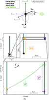 |
Fig. 8. Same as Fig. 4, but with orbits in the polar plane and having a major axis on the equatorial plane of the black hole (see Sect. 4.4.2). We see that the LT effect shifts the apocenter in the counterclockwise direction as seen on this projection. The quadrupole moment effect shifts the apocenter clockwise as seen on the face-on projection of Fig. 4a. |
Overall, this investigation demonstrates that although, in principle, a single randomly oriented orbit contains signatures of all relativistic effects, the relative contributions are often entangled. Observing orbits with diverse orientations provides complementary information and helps to disentangle the in-plane and out-of-plane precession components.
5. Summary and conclusions
In this paper, we present the various kinds of precessions undergone by a stellar orbit due to the 1.5- and 2PN-order spin effects. We show that on an orbital timescale, the orbit frame is subject to an in-plane precession parametrized by the rate  and to out-of-plane precessions parametrized by the rates
  and
and  . Integrating over an orbit, we provide the 2PN expressions of Δϖ, ΔΞ, and ΔΘ, given in Eqs. (38)–(46), which correspond to the tilt angle between two successive pericenters, and to the out-of-plane tilt of the minor and major axes, respectively (see Fig. 3). We also highlight the contributions due to Schwarzschild, LT, and quadrupole effects in these formulas. Moreover, we show how these orbital timescale precessions are linked to the well-known secular timescale precession of the orbital angular momentum around the black hole spin axis. By considering orbital orientations that maximize the various kinds of precessions of the orbit, we have been able to illustrate these findings numerically and show the consistency of our PN orbit-integration code OOGRE with our analytical predictions. We demonstrate that no single orbital configuration is optimal for detecting all relativistic effects simultaneously; instead, a diversity of orbital orientations is essential for disentangling the different types of precessions. We also provide estimates of the on-sky astrometric effects associated to these various precessions for the particular case of the S2 star, as well as for “S2/10”, a hypothetical star on an orbit that is ten times smaller than that of S2. Our results, highlighting the orbital-timescale reorientation of stellar orbits due to the black hole spin, will be very relevant when we are attempting to detect the spin parameter of Sgr A* on S stars at the Galactic center through their astrometric signatures by the GRAVITY instrument. When comparing the Schwarzschild, LT, and quadrupole moment contributions, their relative magnitudes are governed by their PN order:
-
Schwarzschild precession scales as ϵ ∼ 𝒪(v2/c2) (1PN);
-
LT precession as ϵ3/2 ∼ 𝒪(v3/c3) (1.5PN);
-
Quadrupole moment precession as ϵ2 ∼ 𝒪(v4/c4) (2PN).
Here, ϵ = GM/c2p is the small PN parameter. To quantify how these effects change for stars on tighter orbits, we considered “S2/10”. In this case, the PN parameter increases by a factor of 10 (i.e., ϵS2/10 ≈ 10ϵS2). Thus, we saw that all relativistic effects grow significantly stronger at smaller orbital radii and the shorter orbital periods of such stars enable more frequent pericenter and apocenter passages. As a result, secular precessions accumulate more rapidly over a fixed observational time span. For instance, when working with “S2/10” over one period of S2, the angular shifts are increased by a factor ≈300 for the Schwarzschild precession, by a factor 103 for the LT precessions, and by a factor ≈3000 for the quadrupole moment shifts, compared to the star S2. These scaling properties underscore the high scientific value of monitoring stars on tighter orbits, thus offering a powerful probe of both the spin and multipolar structure of Sgr A*.
While this study concentrates on astrometric effects, relativistic dynamics also imprint measurable signatures on radial velocity curves, especially near pericenter passages where Doppler shifts are strongest. Future high-precision instruments such as ERIS and MICADO will enhance this spectroscopic leverage. Nevertheless, astrometry remains essential, as it provides sensitivity throughout the entire orbit and is less dependent on observing stars precisely at pericenter. A combined astrometric–spectroscopic approach will ultimately deliver the most robust constraints on the black hole’s spin parameters.
Our study highlights the importance of identifying and tracking new S stars in the inner regions of the Galactic Center, where relativistic effects are strongest. The next-generation GRAVITY+ (GRAVITY Collaboration 2023) and ERIS (Kravchenko et al. 2023) instruments will significantly enhance the detection and monitoring capabilities, making it possible to refine the orientation of Sgr A* and further test the no-hair theorem. Even if closer-in stars cannot be detected, an alternative approach is to use multi-star fitting with the currently known S stars. Since these stars have different orientations and thus exhibit different types of secular shifts, they can provide additional constraints on both the black hole’s spin magnitude and its orientation. This method has the potential to reduce the required monitoring time needed to test the no-hair theorem. Additionally, a deeper understanding of systematic uncertainties, including the role of stellar perturbations and external mass distributions, will be necessary to interpret high-precision orbital data robustly and provide a more comprehensive picture of the astrophysical environment surrounding Sgr A*.
Acknowledgments
For fruitful discussions we thank our colleagues Laura Bernard, Éric Gourgoulhon, Aurélien Hees and Alexandre Le Tiec, as well as Clifford M. Will.
References
- Alush, Y., & Stone, N. C. 2022, Phys. Rev. D, 106, 123023 [NASA ADS] [CrossRef] [Google Scholar]
- Angélil, R., & Saha, P. 2014, MNRAS, 444, 3780 [CrossRef] [Google Scholar]
- Blanchet, L., & Iyer, B. 2003, Class. Quantum Grav., 20, 755 [Google Scholar]
- Boain, J. R. 2004, A-B-Cs of sun-synchronous orbit mission design, https://hdl.handle.net/2014/37900, 14th AAS/AIAA Space Flight Mechanics Meeting, Maui [Google Scholar]
- Brumberg, V. A. 2017, Essential Relativistic Celestial Mechanics (CRC Press) [Google Scholar]
- Dixon, W. G. 1970, Proc. Roy. Soc. London Ser. A, 314, 499 [Google Scholar]
- Eckart, A., & Genzel, R. 1996, Nature, 383, 415 [NASA ADS] [CrossRef] [Google Scholar]
- EHT Collaboration (Akiyama, K., et al.) 2022, ApJ, 930, L12 [NASA ADS] [CrossRef] [Google Scholar]
- ESO 2025, MICADO – ELT Instrument, https://elt.eso.org/instrument/MICADO, accessed August 2025 [Google Scholar]
- Fabrycky, D., & Tremaine, S. 2007, ApJ, 669, 1298 [NASA ADS] [CrossRef] [Google Scholar]
- Ghez, A. M., Klein, B. L., Morris, M., & Becklin, E. E. 1998, ApJ, 509, 678 [NASA ADS] [CrossRef] [Google Scholar]
- Ghez, A. M., Duchêne, G., Matthews, K., et al. 2003, ApJ, 586, L127 [Google Scholar]
- Ghez, A. M., Salim, S., Weinberg, N. N., et al. 2008, ApJ, 689, 1044 [Google Scholar]
- Gillessen, S., Eisenhauer, F., Trippe, S., et al. 2009, ApJ, 692, 1075 [NASA ADS] [CrossRef] [Google Scholar]
- Gillessen, S., Plewa, P. M., Eisenhauer, F., et al. 2017, ApJ, 837, 30 [Google Scholar]
- Gourgoulhon, E. 2026, Geometry and Physics of Black Holes [Google Scholar]
- GRAVITY Collaboration (Abuter, R., et al.) 2018, A&A, 615, L15 [NASA ADS] [CrossRef] [EDP Sciences] [Google Scholar]
- GRAVITY Collaboration (Abuter, R., et al.) 2020, A&A, 636, L5 [NASA ADS] [CrossRef] [EDP Sciences] [Google Scholar]
- GRAVITY Collaboration (Abuter, R., et al.) 2022, A&A, 657, L12 [NASA ADS] [CrossRef] [Google Scholar]
- GRAVITY Collaboration (Abuter, R., et al.) 2023, The Messenger, 189, 17 [Google Scholar]
- GRAVITY Collaboration (Abd El Dayem, K., et al.) 2024, A&A, 692, A242 [NASA ADS] [CrossRef] [EDP Sciences] [Google Scholar]
- Grould, M., Vincent, F. H., Paumard, T., & Perrin, G. 2017, A&A, 608, A60 [NASA ADS] [CrossRef] [EDP Sciences] [Google Scholar]
- Heißel, G., Paumard, T., Perrin, G., & Vincent, F. 2022, A&A, 660, A13 [NASA ADS] [CrossRef] [EDP Sciences] [Google Scholar]
- Kocsis, B., & Tremaine, S. 2011, MNRAS, 412, 187 [NASA ADS] [CrossRef] [Google Scholar]
- Kocsis, B., & Tremaine, S. 2015, MNRAS, 448, 3265 [NASA ADS] [CrossRef] [Google Scholar]
- Kravchenko, K., Dallilar, Y., Absil, O., et al. 2023, Ground-based and Airborne Instrumentation for Astronomy IX, 121845M [Google Scholar]
- Krishnendu, N. V., Saleem, M., Samajdar, A., et al. 2019, Phys. Rev. D, 100, 104019 [Google Scholar]
- Merritt, D. 2013, Dynamics and Evolution of Galactic Nuclei, Princeton Series in Astrophysics (Princeton: Princeton University Press) [Google Scholar]
- Merritt, D., Alexander, T., Mikkola, S., & Will, C. M. 2010, Phys. Rev. D, 81, 062002 [Google Scholar]
- Poisson, E. 1998, Phys. Rev. D, 57, 5287 [Google Scholar]
- Poisson, E., & Will, C. M. 2014, Gravity: Newtonian, Post-Newtonian, Relativistic (Cambridge: Cambridge University Press) [Google Scholar]
- Psaltis, D., Gongjie, L., & Abraham, L. 2013, ApJ, 777, 57 [Google Scholar]
- Schödel, R., Ott, T., Genzel, R., et al. 2002, Nature, 419, 694 [Google Scholar]
- Tucker, A., & Will, C. 2019, Class. Quantum Grav., 36, 115001 [Google Scholar]
- Waisberg, I., Dexter, J., Gillessen, S., et al. 2018, MNRAS, 476, 3600 [NASA ADS] [CrossRef] [Google Scholar]
- Will, C. M. 2008, ApJ, 674, L25 [NASA ADS] [CrossRef] [Google Scholar]
- Will, C. M. 2018, Theory and Experiment in Gravitational Physics, Second Edition (Cambridge: Cambridge University Press) [Google Scholar]
- Will, C., & Maitra, M. 2017, Phys. Rev. D, 95, 064003 [CrossRef] [Google Scholar]
- Will, C., Naoz, S., Hees, A., et al. 2023, ApJ, 959, 58 [NASA ADS] [CrossRef] [Google Scholar]
- Yu, Q., Zhang, F., & Lu, Y. 2016, ApJ, 827, 114 [NASA ADS] [CrossRef] [Google Scholar]
All reference frames in this paper are right-handed and centered on Sgr A*.
The plane containing the black hole, the star and the three-velocity.
Also denoted as (n, m, k) in Eq. (4.55) of Merritt (2013).
Because it allows to disentangle the LT from the quadrupole moment effects.
We can replace χ by its expression as a function of Q in the analytical expressions of Sect. 4.1.2 to retrieve he analytical expressions as a function of quadrupole moment.
If we want to study circular orbits where e = 0, it is advised to use an alternative set of variables to avoid the null denominator in Eq. (14), as done in Will & Maitra (2017). Here, we consider realistic orbits where e ≠ 0.
This is one way of defining the pericenter advance. Another way to derive the pericenter advance is by directly integrating the timelike geodesic equation which, by means of the conservation of energy and angular momentum, leads to an ordinary differential equation for the radius r in terms of the angle ϕ of the Boyer-Lindquist coordinates (Gourgoulhon 2026; Tucker & Will 2019). The angle between successive turning points, or extrema of r, can be obtained exactly from a radial integral. The expansion of that result in a PN sequence agrees with the osculating element method at lowest order and the differences at higher orders are illusory, because the semilatus rectum and eccentricity have different meanings in the two approaches (Tucker & Will 2019). However, we note that the integration of f from f0 to f0 + 2π is not valid in the case of a “zoom-whirl” behavior (Gourgoulhon 2026).
With the various contributions of the Schwarzschild, LT, and quadrupole moment effects denoted using the “Sch”, “LT”, and “Q” subscripts.
Two flavors of gravitational lensing are implemented in OOGRE: a ray-tracing based one and an analytical approximation; both are turned off in this section.
It is not the exact value of the time of apocenter passage because here  is the osculating (Keplerian) constant and not the relativistic variable.
In the case where we have out-of-plane precession, the notion of in-plane becomes more sensitive, considering that the orbital plane changes all the time. In the following, we use this formulation to refer to instantaneous in-plane precession.
In the second line of equation “(3)” of Will et al. (2023) the unit vector “eX” should be expressed as “eY”.
The evolution of the orbital angular momentum direction makes the notion of face-on or edge-on view of the orbit tricky when θ ≠ 0; therefore, when talking about a face-on or edge-on view of the orbit in this article, we are referring to the initial view of the orbit.
Meaning that the orbit plane contains the spin axis of the black hole or (equivalently) that zorb is perpendicular to zbh. Considering that θ has a periodic variation due to the LT effect in this case, but not a secular one (see Sect. 4.3), a polar orbit will only remain polar on a secular scale.
Which is flattened around the poles.
By using the following definition for the time-average of a quantity F,  .
.
Not to be confused with the longitude of the ascending node.
θ can have periodic variations but no secular ones at the 2PN level.
We know that the quantities  and 𝒲Q2PN, the expressions of which are given in Eqs. (C.8) and (C.9) yield zero for equatorial orbits, i.e., for θ = 0 (mod π). This leads to Eqs. (12) and (13) also yielding zero, meaning that no out-of-plane movement is induced by the BH’s spin. Thus, an initially equatorial orbit will remain so, even in the presence of a spin.
Due to the ever present in-plane precession, the major axis can only instantaneously be polar or equatorial. Here, we refer to the osculating state.
Note: the inclination, ι, we use here is different from the definition of the inclination, "i", used in GRAVITY Collaboration (2020), which was applied in the opposite convention for the sense of rotation of the inclination (see Appendix C of Heißel et al. 2022).
In this paper, all angles are defined according to the right-hand rule; namely, they have positive values when they represent a rotation that appears counterclockwise when looking in the negative direction of the axis, and negative values when the rotation appears clockwise.
When not mentioned, the osculation times of S stars actually correspond to the time of the most recent apocenter before the first observation date of each star, as mentioned in GRAVITY Collaboration (2018, 2000).
In EHT Collaboration (2022), they refer to the spin parameter as "a*" and the black hole inclination with respect to the line of sight as "i". They use the following convention a* ∈ [ − 1; 1] and i ∈ [0; π/2] instead of ours, which aligns with the work of Grould et al. (2017).
Also denoted as (n, m, k) in Eq. (4.55) of Merritt (2013).
The use of θ and β − φ greatly simplifies the scalar products as detailed at the end of Appendix B.
Be aware that in Will & Maitra (2017), Tucker & Will (2019) the quantities "ι", "ω" and "Ω" do not share the same definition as in this paper, in Will (2008, 2018), or in Alush & Stone (2022). For example, their inclination "ι" corresponds to θ in this paper and not ι.
Not to be confused with the varying ϵ.
Note that Will & Maitra (2017), Tucker & Will (2019) call Qα(0) the quantity labeled Qα(1) in these notes. This is because they consider it as a 0PN quantity in  , while we consider it as a 1PN quantity in dX/dφ. The two points of view are exactly equivalent.
Appendix A: Orbit parametrization
Let us present the different ways to parameterize our orbits.
A.1. Newtonian orbits
A Newtonian orbit is defined by six Keplerian parameters that correspond to the 6 Newtonian degrees of freedom (three positions + three velocities). The typical set of Keplerian parameters is the following:
-
asma the semimajor axis;
-
e the eccentricity of the orbit;
-
ι ∈ [0; π] is the inclination21 between the fundamental and orbital planes, and encodes the rotation about ℒorb//sky, from Z to zorb;
-
Ω ∈ [0; 2π] is the position angle of the line of nodes ℒorb//sky, intersection between the orbital and fundamental planes; it encodes the rotation about Z, from X to ℒorb//sky;
-
ω ∈ [0; 2π] is the angular position of the pericenter within the orbital plane, counted from the line of nodes; it encodes the rotation about zorb, from ℒorb//sky to xorb;
-
tperi the time of pericenter passage.
The first two parameters are sufficient to define (i) geometrically the ellipse of the orbit (that is, the semimajor and semiminor axes), and (ii) the energetics of the orbit, that is, the total energy E and angular momentum L of the two-body system. There is a one-to-one correspondence between (asma, e) and (E, L). Note that these parameters are independent of the choice of fundamental frame. In addition, we defined22 the three angles ι, Ω, and ω (see Fig. 1) that encode the orientation of the ellipse; they are the three Euler angles, allowing to rotate the orbit frame into the observer’s frame. We highlight this dependency of the three angular orbital parameters on the choice of fundamental plane. For instance, Will & Maitra (2017) used the black hole equatorial plane as their fundamental plane, while we use the plane of the sky. As a consequence, the inclination angle of our work is not the same as in theirs, and we can see that this has obviously profound consequences on the evolution equations that we end up obtaining. Moreover, we need the initial condition along the orbit, so we introduce tperi the time of pericenter passage. Finally, to characterize the position of the star along the orbit, we use the true anomaly f (see Fig. 1) or the azimuthal angle φ = ω + f.
A.2. Relativistic orbits
For orbits considered in the framework of GR or PN theories, the orbital elements become time-varying. The values of the orbital parameters at a particular date can thus be seen as the orbital parameters of a Newtonian orbit, osculating the relativistic orbit at this particular date. It is customary to represent a relativistic orbit by providing the set of orbital parameters at a particular time, tosc, when it is osculated by the Newtonian orbit described by this same set of orbital parameters. A relativistic orbit is thus described by the six usual orbital parameters, plus the osculating time tosc. The time-varying orbital parameters of a relativistic orbit can therefore be seen as the orbital parameters of a family of osculating Newtonian elliptical orbits. From this point onward, we consider (asma, e, ι, Ω, ω) as functions of time such that (asma(tosc), e(tosc), ι(tosc), Ω(tosc), ω(tosc)) = (asma, osc, eosc, ιosc, Ωosc, ωosc).
As for the osculating tperi, we take the most recent time of pericenter passage before the first observation date of each star (see table D.1 of GRAVITY Collaboration 2022, for the first observation dates).
Moreover, it is worth mentioning that adding a certain time T to tosc does not mean that the orbit would be temporally translated by T; taking tosc = t0 + T instead of tosc = t0 does not mean that we would observe the same orbit if we wait for T. This would only be true if we also add T to tperi as well. Since it is common not to find in literature23 any mention of the osculating time when giving the numerical values of the orbital parameters of S stars, we could possibly end up misinterpreting the true values of these parameters (see Heißel et al., in prep.).
Finally, it is very important to realize that the same set of initial conditions will yield different GR orbits when using different coordinate systems. This is well known in the context of relativity theory and stems from the fact that orbital elements are not covariant quantities (Brumberg 2017). Therefore, a relativistic orbit should be described by a set of 6 orbital parameters, plus the osculating time, plus the mention of the coordinate system used in the integration. This information is necessary and sufficient for uniquely pinpointing the orbit (see Heißel et al., in prep.).
Appendix B: Details on the frames of reference
In this appendix, we gather some details about the frames of reference of Sect. 2, that are important for the comprehension and reproducibility of our results. First, concerning the orbit frame represented in Fig. 1, we define the line of nodes as the intersection between the orbit and sky planes, and its director vector ℒorb//sky goes from the black hole to 𝒜𝒩orb//sky, the ascending node of the orbit with respect to the observer. The latter is the intersection between the sky plane and trajectory where the star passes from behind the sky plane (Z < 0) to the front (Z > 0).
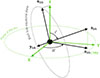 |
Fig. B.1. Angles (i′,Ω′) in black characterize the spin orientation of Sgr A* and give the position of the black-hole frame relative to the observer frame. |
Second, concerning the black hole frame, we mentioned that the choice of the orientation of xbh and ybh inside the black hole equatorial plane has no impact on the physics of the problem.
We have defined in Fig. 2 the orientation of zbh in the orbit frame by introducing the angles (θ, β). These angles are very useful for simplifying the computations of the quantities appearing in Lagrange planetary equations. Here we introduce an alternative definition with the angles24 (i′,Ω′) defined in Fig. B.1. These angles are more adapted when dealing with multi-star fit because they allow us to characterize the orientation of the black hole with respect to the observer we use the angles (i′,Ω′). This is particularly useful in the case of studying the spin of SgrA*; multiple stars would be used when constraining the spin and its orientation, meaning that defining the latter with respect to the orbit of one single star instead of the sky is unpractical. On the other hand, for the calculations presented in Sect. 3.2, the use of (θ, β), which define the orientation of the spin vector relative to the star’s orbit and ℒorb//sky, would be more practical. This allows us to define the black hole’s angles with respect to the sky plane as follows:
-
i′∈[0; π] is the rotation angle from Z to zbh;
-
Ω′∈[0; 2π] is the rotation angle about Z, from X to zbh//sky.
Third, we introduced in Fig. 1 the Gaussian frame (norb, morb, zorb)25. This allows us to write the star’s velocity vector v of norm v as
 (B.1)
(B.1)
with
 (B.2)
(B.2)
This can be done, even in the presence of an "out-of-plane precession" (see Sect. 3) since at any time, we can consider the osculating Keplerian orbit (see Sect. 3) which contains the velocity of the star at that time. In other words, the velocity is always within the momentarily orbital plane, and thus never has a zorb-component. In addition to the true anomaly f introduced in Sect. 2, it is also useful to define the angle φ = ω + φ ∈ [0; 2π], defined as the rotation angle about zorb, from ℒorb//sky to norb, and characterizing the position of the star along the orbit relative to the ascending note (see Fig. 1). We know from Eq. (4.55) of Merritt (2013) that by defining this quantity we can write
 (B.3)
(B.3)
Similarly to the expression of zorb, we can write zbh in the fundamental frame of the observer as
 (B.4)
(B.4)
Therefore, we obtain
 (B.5)
(B.5)
These expressions are very handy for the derivation of Eqs. (C.1) to (C.9).
Appendix C: Perturbations in the Gaussian frame
Let us express26 the components of the various PN accelerations in the Gaussian frame (norb, morb, zorb):
 (C.1)
(C.1)
 (C.2)
(C.2)
 (C.3)
(C.3)
 (C.4)
(C.4)
 (C.5)
(C.5)
 (C.6)
(C.6)
 (C.7)
(C.7)
![Mathematical equation: $$ \begin{aligned} \mathcal{W} _{\mathrm{LT} }^{\mathrm{1.5PN} } =&\mathbf a _{\rm LT}^{\mathrm{1.5PN} } \cdot \mathbf z _{\mathrm{orb} }\nonumber \\ =&2\epsilon ^{3/2}\frac{Gm}{p^{2}} \chi (1+e\cos f)^3\sin \theta \nonumber \\&\times \left[ 2(1+e\cos f)\cos (\beta -\varphi ) +e\sin f\sin (\beta -\varphi ) \right];\end{aligned} $$](/articles/aa/full_html/2026/03/aa55753-25/aa55753-25-eq120.gif) (C.8)
(C.8)
 (C.9)
(C.9)
Appendix D: Secular evolution in the PN formalism and two-timescale analysis
It is possible to derive the secular evolution of the orbital parameters at an arbitrary PN order using a perturbation method called two-timescale analysis. This section tries to pedagogically introduce the material presented in Will & Maitra (2017), Tucker & Will (2019), while taking the orbital elements as the ones defined with respect to observer’s frame and not the black hole’s frame27; this allows us to obtain secular shifts of quantities that are directly observable.
D.1. Two-timescale method
Let us label generically all orbital elements by Xα, where α is an index, running typically from 1 to 5 to label the 5 standard orbital elements (p, e, ι, Ω, ω). Here, we use the orbital plane azimuthal angle φ = ω + f as the parameter, rather than time. So we consider functions Xα(φ). Equations (10) to (14) give the time evolution dXα/dt. By using Eq. (15) we can easily get
 (D.1)
(D.1)
and convert dXα/dt to dXα/dφ. The expressions of the various perturbing accelerations up to 2PN order are given by Eqs. (C.1) to (C.9).
Finally, using all this material, the evolution of the orbital elements is expressed as
 (D.2)
(D.2)
where we express the PN small parameter28
 as
as
 (D.3)
(D.3)
Here, we use an orbit-averaged value of the semilatus rectum,  , which is constant in the evolution. The functions
  ,
,  , and
, and  , denote the 1PN, 1.5PN, and 2PN components of the evolution equation, respectively, and the Qα(i) are by definition 0PN quantities.
The evolution of the orbital parameters under these PN components takes the form of a long-term (compared to the orbital period) secular evolution, on top of which there are quickly-varying (at the orbital timescale) oscillations. Such a behavior can be well captured in the framework of a two-timescale analysis. Based on this understanding of what the solution should look like, we consider that Xα is no longer a function Xα(φ) of the orbital plane azimuthal angle, but rather a function of two variables, Xα(Φ, φ), where  captures the long-term behavior of the element, while φ captures the quickly-varying oscillations. We use the trick of considering that φ and Φ are independent variables (which is only a trick, they are actually directly related by
  ), and derive evolution equations for Xα, now considered as a function of two independent variables Φ and φ.
Let us rewrite with more details the evolution of Xα, which now reads
 (D.4)
(D.4)
where we recall that  does not depend on any variable quantity, and Qα(1), Qα(3/2) and Qα(2) now depend on the various orbital parameters considered as functions of two variables, Xβ(Φ, φ), and explicitly also on φ. Next, we look for a solution that is expressed as
 (D.5)
(D.5)
where  captures the long-term, secular evolution of the orbital element, while Yα(i) capture the quickly-varying evolution due to the different perturbing accelerations, the upper index i reminding the PN order of the small oscillating correction to the secular evolution. We assume that these Yα(i) are 2π-periodic in φ.
There is not unicity of this ansatz of solution but it is natural to consider
 (D.6)
(D.6)
where
 (D.7)
(D.7)
is the orbit average of some function F(Φ, φ), where we consider that Φ remains constant in the average, and that the result does not depend on the value of Φ. So we consider that  is simply the orbit average of Xα, and that the oscillating term Yα(i) averages to zero over one orbit. Now that we have this ansatz of the solution, we can rewrite the evolution of the orbital parameter, Xα. We express the derivative with respect to Φ as
 (D.8)
(D.8)
and Eq. (D.4) becomes
 (D.9)
(D.9)
Using  and dividing by
  , we get
 (D.10)
Here, we keep in mind that we have divided by  , so a term of order kPN in dXα/dφ is then on the order of (k − 1)PN in
  .
.
We know that
![Mathematical equation: $$ \begin{aligned} \left\langle \frac{\partial Y^{(i)}_\alpha }{\partial \varphi } \right\rangle = \frac{1}{2\pi } \int _0^{2\pi } \frac{\partial Y^{(i)}_\alpha }{\partial \varphi } d \varphi = \frac{1}{2\pi } \left[Y^{(i)}_\alpha \right]_0^{2\pi } = 0, \end{aligned} $$](/articles/aa/full_html/2026/03/aa55753-25/aa55753-25-eq146.gif) (D.11)
(D.11)
considering that Yα(i) is 2π-periodic. Also, if we assume that Φ and φ are independent, we can write
 (D.12)
where we use the standard coma notation for partial derivatives. Then,
 (D.13)
and by taking the orbit average, we get
 (D.14)
Let us now consider the Taylor expansions:
 (D.15)
where the same coma notation for partial derivative is used. The summation is done on all parameters  that appear in Qα(i). Note that
  in this expression means that we consider the orbital parameters to be only secularly varying, and constant at the orbital timescale considered in the average process. So considering all terms up to 1PN order, Eq. (D.14) becomes
![Mathematical equation: $$ \begin{aligned} \frac{\mathrm{d} \tilde{X}_\alpha (\Phi )}{\mathrm{d} \Phi } =&\langle Q_\alpha ^{(1)}(\tilde{X}_\beta ;\varphi ) \rangle \nonumber \\&+ {\tilde{\epsilon }}^{1/2}\langle Q_\alpha ^{(3/2)} (\tilde{X}_\beta ;\varphi ) \rangle \nonumber \\&+ \tilde{\epsilon } \left[\sum _\gamma \left(\langle Y^{(1)}_\gamma \, Q_{\alpha ,\gamma }^{(1)} (\tilde{X}_\beta ;\varphi ) \rangle \right) + \langle Q_\alpha ^{(2)}(\tilde{X}_\beta ;\varphi ) \rangle \right]. \end{aligned} $$](/articles/aa/full_html/2026/03/aa55753-25/aa55753-25-eq153.gif) (D.16)
(D.16)
This is the final expression of the secular evolution of the orbital parameters. This expression is in agreement with the formulas of Will & Maitra (2017), Tucker & Will (2019) provided that only Qα(1) is considered29. Will & Maitra (2017), Tucker & Will (2019) derive the following expression for Yα(1):
 (D.17)
The first term in the square brackets of Eq. (D.16) then becomes
 (D.18)
so that provided that the Qα(i) are known for all elements, the secular evolution can be derived. Finally we can come back to the evolution equation as a function of φ by remembering that Φ and φ are actually the same quantity up to a factor  . So we get
![Mathematical equation: $$ \begin{aligned} \frac{\mathrm{d} \tilde{X}_\alpha (\varphi )}{\mathrm{d} \varphi } =&\tilde{\epsilon } \, \langle Q_\alpha ^{(1)}(\tilde{X}_\beta ;\varphi ) \rangle \nonumber \\&+ {\tilde{\epsilon }}^{3/2} \, \langle Q_\alpha ^{(3/2)} (\tilde{X}_\beta ;\varphi ) \rangle \nonumber \\&+ {\tilde{\epsilon }}^{2} \left[\sum _\gamma \left(\langle Y^{(1)}_\gamma \, Q_{\alpha ,\gamma }^{(1)} (\tilde{X}_\beta ;\varphi ) \rangle \right) + \langle Q_\alpha ^{(2)}(\tilde{X}_\beta ;\varphi ) \rangle \right], \end{aligned} $$](/articles/aa/full_html/2026/03/aa55753-25/aa55753-25-eq157.gif) (D.19)
(D.19)
which is the second order secular evolution of the orbital element, here considered as a function of φ only (the variable Φ was just a mathematical trick to derive the equation).
D.2. Application to the 2PN Schwarzschild shift
In this section we neglect the spin effects and consider a 2PN Schwarzschild spacetime. So in particular the Qα(3/2) is zero.
Let us start from the expression of dω/dt given in Eq. (14). Equation (D.1) leads to
 (D.20)
as Ω is constant in Schwarzschild (the evolution of Ω depends on 𝒲, which is linked to the spin). The evolution of ω as a function of φ then reads
![Mathematical equation: $$ \begin{aligned} \frac{\mathrm{d} \omega }{\mathrm{d} \varphi } =&\frac{1}{e} \sqrt{\frac{p}{GM}} \left[- \cos f \mathcal{R} + \frac{2 + e \cos f}{1 + e \cos f} \sin f \mathcal{S} \right]\nonumber \\&\times \sqrt{\frac{p^3}{GM}} \left(1 + e \cos f\right)^{-2}, \end{aligned} $$](/articles/aa/full_html/2026/03/aa55753-25/aa55753-25-eq159.gif) (D.21)
(D.21)
by combining Eqs. (10) to (14) and (D.20). Using the 2PN expressions of ℛ and 𝒮 given in Eqs. (C.1) and (C.4), we get
![Mathematical equation: $$ \begin{aligned} \frac{\mathrm{d} \omega }{\mathrm{d} \varphi }&= \epsilon \, \frac{1}{e} \left[-\cos f \left(3 + 2 e \cos f + e^{2} \left(4 \sin ^{2} f - 1\right)\right)\right.\nonumber \\&\qquad \;\left.+ 4\, \frac{2 + e \cos f}{1 + e \cos f} \sin f \left(1 + e \cos f\right) e \sin f\right]\nonumber \\&+ \epsilon ^{2} \, \frac{1}{e} \left[-\cos f \left(- 9 \left(1 + e \cos f\right)^{2} \right)\right.\nonumber \\&\qquad \;\left.- 2 \, \frac{2 + e \cos f}{1 + e \cos f} \sin f\left(1 + e \cos f\right)^{2} \, e \sin f\right]. \end{aligned} $$](/articles/aa/full_html/2026/03/aa55753-25/aa55753-25-eq160.gif) (D.22)
(D.22)
We want to replace ϵ by  , for a constant value of the semilatus rectum
  to obtain
![Mathematical equation: $$ \begin{aligned} \frac{\mathrm{d} \omega }{\mathrm{d} \varphi }&= \tilde{\epsilon } \, \frac{1}{e} \, \frac{\tilde{p}}{p}\, \left[-\cos f \left(3 + 2 e \cos f + e^{2} \left(4 \sin ^{2} f - 1\right)\right)\right.\nonumber \\&\qquad \;\left.+ 4\, \frac{2 + e \cos f}{1 + e \cos f} \sin f \left(1 + e \cos f\right) e \sin f\right]\nonumber \\&+ {\tilde{\epsilon }}^{2} \, \frac{1}{e} \left(\frac{\tilde{p}}{p}\right)^{2} \left[-\cos f \left(- 9 \left(1 + e \cos f\right)^{2}\right)\right.\nonumber \\&\qquad \;\left.- 2 \, \frac{2 + e \cos f}{1 + e \cos f} \sin f \left(1 + e \cos f\right)^{2} \, e \sin f\right], \end{aligned} $$](/articles/aa/full_html/2026/03/aa55753-25/aa55753-25-eq163.gif) (D.23)
(D.23)
which takes the exact same form as the general expression of Eq. (D.4). The quantity in factor of  in the first line corresponds to Qω(1), while that in factor of
  in the second line corresponds to Qω(2). They both depend on three orbital parameters, ω itself (through f = φ − ω), p and e, as well as explicitly on φ (again through f). They are 2π-periodic in φ. Let us simplify a bit to get
 (D.24)
We now want to compute Eq. (D.19) for ω, which reads
![Mathematical equation: $$ \begin{aligned} \frac{\mathrm{d} \tilde{\omega }}{\mathrm{d} \varphi }&= \tilde{\epsilon } \, \left\langle Q_\omega ^{(1)}(p, e,\omega ,\varphi ) \right\rangle \nonumber \\&+ {\tilde{\epsilon }}^{2} \left[\left\langle Y^{(1)}_p \, Q_{\omega ,p}^{(1)} (p, e,\omega ,\varphi ) \right\rangle + \left\langle Y^{(1)}_e \, Q_{\omega ,e}^{(1)} (p, e,\omega ,\varphi ) \right\rangle \right.\nonumber \\&\qquad \;\left.+ \left\langle Y^{(1)}_\omega \, Q_{\omega ,\omega }^{(1)} (p, e,\omega ,\varphi ) \right\rangle + \,\left\langle Q_\omega ^{(2)} (p, e,\omega ,\varphi ) \right\rangle \right], \end{aligned} $$](/articles/aa/full_html/2026/03/aa55753-25/aa55753-25-eq167.gif) (D.25)
(D.25)
where we remind that the orbital elements appearing in the various functions Q and Y are considered to vary only secularly (see the comment following Eq. (D.15)): they are functions of Φ alone, they do not depend on φ, so they are not affected by the orbit averaging. For instance, we have ⟨e cos f⟩ = e⟨cos f⟩, which would not be true if the full dependence of e on both φ and Φ was considered.
The first and last terms of Eq. (D.25) are trivial to compute
 (D.26)
where we use  , which is true here given that the orbital-timescale variability of p is discarded, only its secular variation is considered.
The value of ⟨Qω(1)⟩ leads to the well-known textbook result:  at 1PN order. However here, we need to go to 2PN, so a we also need to consider the three ⟨YQ⟩ terms in the bracket of Eq. (D.25). These are expressed as
 (D.27)
where we use Eq. (D.18) to express the Yα(1). We thus need to compute quite a few more terms. Let us start by:
 (D.28)
The last two have zero average, because ⟨cos f⟩ = ⟨sin f⟩ = ⟨cos f sin f⟩ = 0. So, this cancels a few terms in the second and third lines of the RHS of Eq. (D.27). Following the exact same procedure as for ω, we can write dp/dφ and de/dφ, and extract their 1PN component to get
 (D.29)
both of which have zero average (no secular evolution of p and e at 1PN order). This cancels the first two terms of the last two lines in Eq. (D.27). So we are left with:
 (D.30)
It is easy to get
 (D.31)
using
 (D.32)
The terms with integrals of Qβ(1) are a bit more cumbersome, but it is still straightforward to obtain
 (D.33)
Putting everything together, we finally arrive at
 (D.34)
Equation (D.34) reproduces the 2PN result of Will & Maitra (2017), see their Eq. (3.23a). To obtain the secular pericenter shift, we must integrate over a full radial cycle (f : 0 → 2π) rather than a full azimuthal cycle (φ : 0 → 2π), since in the PN regime the pericenter itself precesses. We expand the argument of pericenter as
 (D.35)
with ϵ0 = GM/(p0c2) the PN small parameter. At first post-Newtonian order, we find
 (D.36)
so that over a full radial period,
 (D.37)
Combining Eq. (D.37) with Eq. (D.34), the 2PN pericenter advance in Schwarzschild spacetime reads
 (D.38)
where the substitution  introduces only 3PN-level corrections. Thus, the final expression for the 2PN secular shift of the pericenter/apocenter is
 (D.39)
Here, the quantities  and
and  refer to orbit-averaged parameters. If, in the 2PN term of Eq. (D.39), we replace
  and
and  with their osculating counterparts ϵosc = ϵ(posc) and eosc, this substitution would only modify the result at 3PN order–meaning the 2PN expression remains unchanged. However, replacing
  with ϵosc in the 1PN term would already introduce a discrepancy at 2PN order.
This is why, when expressing the pericenter advance to 2PN accuracy, it is essential to keep the orbit-averaged quantity  in the 1PN term (
 and not 6πϵosc). Alternatively, if the preference is to work with osculating elements throughout, the entire perturbative approach–including the ansatz for the solution (e.g., Eq. (D.6))–must be adjusted accordingly. In that case, the expression for the 2PN pericenter advance would take a different form, reflecting the difference in parameterization.
In contrast, for the 2PN-order secular shifts due to the LT effect and the black hole’s quadrupole moment, the expressions involve only leading-order contributions. Therefore, we could safely use either averaged or osculating values of p, θ, and ψ without affecting the accuracy at the given order.
Appendix E: Mid-inclined orbits
We investigate the case of a mid-inclined orbit, for example, the case where  , namely, (θ, ψ) = (π/4, 3π/2) or (θ, ψ) = (3π/4, π/2). we see from Eqs. (39), (42), and (45) that with these values of θ and ψ, we end up observing both in-plane and out-of-plane precessions due to the LT effect, at moderate values. However, when looking at Eqs. (43) and (46) we see that the orbits will experience the most out-of-plane shift due to the quadrupole moment in this configuration. Indeed, when simulating a prograde and retrograde orbit relative to the black hole, we see in Figs. E.1 and E.2 that the LT and quadrupole moment effects each make the apocenters experience both an in-plane and out-of-plane precession. The in-plane precessions are similar the the equatorial orbit case. As for the out-of-plane precessions, they mainly act on the major axis but also on the minor axis on much longer timescales (see Eq. (E.1) below). We also see that the quadrupole moment appears to oppose the LT effect for the out-of-plane shift when the orbit is prograde, but not for the retrograde orbit.
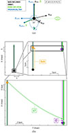 |
Fig. E.1. Same as Fig. 4, but with mid-inclined orbits relative to the equatorial plane of the black hole. We see that that the apocenter experiences both an in-plane and out-of-plane precession due to the LT effect. The in-plane precession is clockwise as seen on the face-on projection of Fig. 4a, and the out-of-plane precession is mainly for the major axis but also acts on the minor axis. We also see that the quadrupole moment appears to have the opposite behavior to the LT effect for both the in-plane and out-of-plane shifts. |
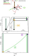 |
Fig. E.2. Same as Fig. E.1, but for retrograde orbits, relative to the black hole. We see that the apocenter experiences both an in-plane and out-of-plane precession due to the LT effect. The in-plane precession is clockwise as seen on the face-on projection of Fig. 5a, and the out-of-plane precession is mainly for the major axis, but also acts on the minor axis. We also see that the quadrupole moment appears to have the same behavior as the LT effect for the both types of precession. |
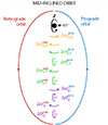 |
Fig. E.3. Schematic illustration of the secular precessions for a mid inclined orbit relative to the equatorial plane of the black hole. When we have |

In practice, unless we have an equatorial (no out-of-plane precession) or polar (surface of the out-of-plane precession cone represented in Fig. 3 being a plane for θ = π/2 (mod π)) orbit with the major axis being equatorial or polar, both the major and minor axis will precess. However, the out-of-plane shift remains mainly along the tangent to the surface of the out-of-plane precession cone as long as the period of the orbit is much less than the precession period Pcone of the angular momentum of the orbit around the out-of-plane precession cone. To check that, we derive Pcone/P using Eqs. (49) and (56) at the 2PN order, expressed as
 (E.1)
(E.1)
If we apply this estimation for "S2/10" for example, we get  ,
,  ,
,  and
and  .
.
In Fig. E.3, we summarize in a schematic way the results of Figs. E.1 and E.2 and consider how the quadrupole moment out-of-plane precession of the major axis, is studied through a mid-inclined orbits with zbh//orb//yorb. Alternatively, in order to maximize the quadrupole moment out-of-plane precession of the minor axis instead of the major axis, we would need to study a mid-inclined orbits with zbh//orb//xorb.
In conclusion, we now have insight into the different types of precession that can manifest around a rotating black hole and comprehend how a random relative orientation between the orbit and black hole can be decomposed into these precession categories. With this new understanding, we can have a better understanding of the possible black hole orientations that can generate the secular precessions that observed for the orbits of currently, and potential closer-in stars.
All Tables
All Figures
|
Fig. 1. Orbit frame (xorb, yorb, zorb) and orbital elements are represented in purple, while the fundamental frame (X, Y, Z) is in green. The pericenter, represented by the point 𝒫, is also added. Finally, ℒorb//sky denotes the line of nodes of the orbit frame and sky plane. We also represent the Gaussian frame of the star (norb, morb, zorb), the projection of the X axis on the orbit plane denoted by X//orb and the angle, ϖ, introduced in Sect. 4. Here, we illustrate the fundamental frame when it matches that of a distant observer (see Sect. 2). Also, it is useful to note the the azimuthal angle is φ = ω + f. |
| In the text | |
|
Fig. 2. Angles (θ, β) in purple characterize the orientation of the spin vector, zbh, relative to the orbit frame. We also added the angle ψ ≡ β − ω, so that (θ, ψ) are the spherical coordinates of the spin axis in the orbit frame. The projection of zbh on the orbit plane is denoted by zbh//orb. |
| In the text | |
|
Fig. 3. Figure 3a shows the evolution of the orbit orientation on an orbital period P timescale. Three precessions are experienced: an in-plane precession (left panel) with contributions at 1PN, 1.5PN, and 2PN; and two out-of-plane precessions, namely, one around the minor axis (middle panel) and another around the major axis (right panel) with contributions at 1.5PN and 2PN. Figure 3b shows the evolution of the orbit orientation on a secular timescale Pcone ≫ P (see Eq. (E.1)). The orbital angular momentum experiences a precession around the black hole spin axis. |
| In the text | |
|
Fig. 4. Prograde orbits in the equatorial plane of the black hole with a face-on view. Figure 4a displays a schematic illustration of the osculating Keplerian orbit (see Sect. 4.4.1) with the apocenter represented by the letter 𝒜. In Fig. 4b we show an orbit of the hypothetical star “S2/10” simulated in 2PN using OOGRE: the “✷” denotes the apocenters (the first apocenter in black corresponds to the osculating time, which is also the initial date, and is in common for the three orbits). We simulate one orbit for the Schwarzschild precession (“Sch” in orange), one orbit for both the Schwarzschild and LT precessions (“LT” in green), and one orbit for the Schwarzschild, spin and quadrupole moment precessions (“Q” in thin purple). We see that the LT and quadrupole moment effects shift the apocenter clockwise and counterclockwise, respectively, as seen by this face-on observer. All numbers are expressed in mas except otherwise noted. |
| In the text | |
|
Fig. 5. Same as Fig. 4, but for retrograde orbits. We see that both the LT and quadrupole moment effects shift the apocenter clockwise as seen by this face-on observer. |
| In the text | |
|
Fig. 6. Schematic illustration of the secular precessions for a prograde and a retrograde equatorial orbit. We note that Schwarzschild precession and quadrupole moment effect push the apocenter in the direction of stellar motion and the LT precession pushes against the spin. |
| In the text | |
|
Fig. 7. Same as Fig. 4, but with orbits in a polar plane and having a major axis on the spin axis of the black hole (see Sect. 4.4.2). We see that the LT effect shifts the minor axis in the same direction as the the spin of the black hole, gradually shifting the orbit plane from edge-on towards face-on. The quadrupole moment effect shifts the apocenter clockwise as seen on face-on projection of Fig. 4a. |
| In the text | |
|
Fig. 8. Same as Fig. 4, but with orbits in the polar plane and having a major axis on the equatorial plane of the black hole (see Sect. 4.4.2). We see that the LT effect shifts the apocenter in the counterclockwise direction as seen on this projection. The quadrupole moment effect shifts the apocenter clockwise as seen on the face-on projection of Fig. 4a. |
| In the text | |
|
Fig. B.1. Angles (i′,Ω′) in black characterize the spin orientation of Sgr A* and give the position of the black-hole frame relative to the observer frame. |
| In the text | |
|
Fig. E.1. Same as Fig. 4, but with mid-inclined orbits relative to the equatorial plane of the black hole. We see that that the apocenter experiences both an in-plane and out-of-plane precession due to the LT effect. The in-plane precession is clockwise as seen on the face-on projection of Fig. 4a, and the out-of-plane precession is mainly for the major axis but also acts on the minor axis. We also see that the quadrupole moment appears to have the opposite behavior to the LT effect for both the in-plane and out-of-plane shifts. |
| In the text | |
|
Fig. E.2. Same as Fig. E.1, but for retrograde orbits, relative to the black hole. We see that the apocenter experiences both an in-plane and out-of-plane precession due to the LT effect. The in-plane precession is clockwise as seen on the face-on projection of Fig. 5a, and the out-of-plane precession is mainly for the major axis, but also acts on the minor axis. We also see that the quadrupole moment appears to have the same behavior as the LT effect for the both types of precession. |
| In the text | |
|
Fig. E.3. Schematic illustration of the secular precessions for a mid inclined orbit relative to the equatorial plane of the black hole. When we have |
| In the text | |
Current usage metrics show cumulative count of Article Views (full-text article views including HTML views, PDF and ePub downloads, according to the available data) and Abstracts Views on Vision4Press platform.
Data correspond to usage on the plateform after 2015. The current usage metrics is available 48-96 hours after online publication and is updated daily on week days.
Initial download of the metrics may take a while.