| Issue |
A&A
Volume 707, March 2026
|
|
|---|---|---|
| Article Number | A19 | |
| Number of page(s) | 11 | |
| Section | Astrophysical processes | |
| DOI | https://doi.org/10.1051/0004-6361/202556040 | |
| Published online | 25 February 2026 | |
Excitation of the nonresonant streaming instability around sources of ultrahigh-energy cosmic rays
1
Gran Sasso Science Institute (GSSI) Viale Francesco Crispi 7 67100 L’Aquila, Italy
2
INFN-Laboratori Nazionali del Gran Sasso (LNGS) Via G. Acitelli 22 67100 Assergi (AQ), Italy
★ Corresponding author: This email address is being protected from spambots. You need JavaScript enabled to view it.
Received:
20
June
2025
Accepted:
4
January
2026
Abstract
Aims. The interpretation of the ultrahigh-energy cosmic-ray (UHECR) spectrum and composition suggests a suppression of the flux below ≈1 EeV, as observed by the Pierre Auger Observatory and Telescope Array. A natural explanation for this phenomenon involves magnetic confinement effects. We investigate the possibility that UHECRs self-generate the magnetic turbulence necessary for this confinement via current-driven plasma instabilities.
Methods. Specifically, we show that the electric current produced by escaping UHECRs can excite a nonresonant streaming instability in the surrounding plasma. This instability reduces the diffusion coefficient in the source environment and effectively traps particles with energies E ≲ 1 EeV ℒ443/4 RMpc−3/2λ30 for times that exceed the age of the Universe. Here, ℒ44 is the source luminosity in units of 1044 erg/s, RMpc is the radial size in Mpc, and λ30 is the intergalactic magnetic field coherence length in units of 30 Mpc. We discuss the conditions in detail (the source luminosity, the initial magnetic field, and the environment in which this complex phenomenon occurs) that need to be fulfilled in order for self-confinement to take place near a source of UHECRs, and we also discuss the caveats that affect our conclusions. We emphasize that these conclusions were derived within a simplified model framework; their wider applicability requires that the assumptions hold in realistic source environments.
Results. By modeling a population of UHECR sources with a luminosity function typical of extragalactic gamma-ray sources, we connected the spectrum of escaping particles to the luminosity distribution. Furthermore, we calculated the contribution of these confined particles to cosmogenic neutrino production and found consistency with current observational constraints. Our results suggest that self-induced turbulence might play an important role in shaping the UHECR spectrum. In particular, it might account for the flux suppression near their sources. This offers a promising framework for interpreting current observations.
Key words: astroparticle physics / neutrinos / cosmic rays
© The Authors 2026
 Open Access article, published by EDP Sciences, under the terms of the Creative Commons Attribution License (https://creativecommons.org/licenses/by/4.0), which permits unrestricted use, distribution, and reproduction in any medium, provided the original work is properly cited.
This article is published in open access under the Subscribe to Open model. This email address is being protected from spambots. You need JavaScript enabled to view it. to support open access publication.
1. Introduction
The observed spectrum and composition of ultrahigh-energy cosmic rays (UHECRs) as measured by the Pierre Auger Observatory (Auger; Abreu et al. 2021; Aab et al. 2020) provide invaluable insights into their origin. The distribution of the depth of the shower maximum (Xmax; Aab et al. 2014a,b, 2016) reveals information about primary particle types, while spectrum fits, which account for the source evolution and propagation effects (Aab et al. 2017; Abdul Halim et al. 2023), constrain key source parameters such as the spectral shape and elemental composition.
Several robust conclusions have emerged from these fits. We list them below. (1) Above the second knee, UHECRs transition from a mix of protons and medium-mass nuclei (e.g., nitrogen) to a predominantly mixed composition near the ankle (≈1018.3 eV). (2) At energies ≳1019 eV, the absence of a light component implies that the maximum source rigidity is limited to R ≲ 1019 V, which relaxes the demands in terms of acceleration models (Bergman 2006; Shinozaki & Teshima 2004). (3) The inferred source spectrum is unusually hard, with slopes γ ≲ 1. This result is inconsistent with the γ ≳ 2 expected from standard acceleration models such as diffusive shock acceleration at nonrelativistic and relativistic shocks (Blandford & Ostriker 1978; Blandford & Eichler 1987; Sironi et al. 2015). Although they are unusual, these hard spectra have been found in some acceleration models, such as rapidly spinning neutron stars (Blasi et al. 2000; Arons 2003; Kotera et al. 2015), second-order stochastic acceleration in gamma-ray bursts (Asano & Mészáros 2016), and reconnection events in relativistic plasmas (Zhang et al. 2023). More recent Auger data analyses even suggest inverted source spectra (γ < 0) above the ankle, which contradicts existing astrophysical models (Abdul Halim et al. 2023). Furthermore, to reproduce observables below the ankle, an additional soft-spectrum component (γ ≈ 3.5) is needed, which is consistent with measurements of the proton spectrum by KASCADE-Grande (Kang 2023) and IceTop (Aartsen et al. 2019).
A natural interpretation of these findings invokes confinement of UHECRs with energies below the ankle. This scenario can be realized in two main classes of models. (1) Confinement around the sources: In this scenario, heavy nuclei experience energy-dependent confinement in the vicinity of the source or even inside the source. Their prolonged residence time enhances photo-disintegration processes, which alters the observed composition and spectrum (Unger et al. 2015; Muzio et al. 2022). (2) Magnetic horizon effect: Here, the delayed arrival of low-energy particles is attributed to diffusion in strong extragalactic magnetic fields (≳10 nG). This results in an effective low-energy cutoff that depends on the strength and structure of the intergalactic magnetic field (IGMF) (Aloisio & Berezinsky 2004; Mollerach & Roulet 2013; Abdul Halim et al. 2024). Both models require specific assumptions about the source environment or the IGMF. In particular, the latter demands field strengths near the observational upper limits imposed by radio synchrotron and Faraday rotation measurements (Amaral et al. 2021; Carretti et al. 2022).
A third possibility that was originally proposed by Blasi et al. (2015) involves the generation of self-induced turbulence. The electric current carried by escaping UHECRs drives a nonresonant streaming instability (Bell 2004; Amato & Blasi 2009; Bell et al. 2013), which amplifies small-scale magnetic perturbations. These perturbations grow nonlinearly and saturate at scales that are comparable to the gyro-radius of the dominant particles in the current. This mechanism modifies UHECR transport near the source and effectively confines particles and regulates their escape. This situation is similar to the one pictured for the Bell instability taking place at SNR shocks (Bell et al. 2013). Notably, Blasi et al. (2015) demonstrated that for a source luminosity of ℒ ≈ 1044 erg/s, this self-confinement mechanism can trap particles at sub-EeV energies for timescales exceeding the typical source lifetime of ≈10 Gyr.
We build upon this last model and explore four critical aspects. We list these aspects below. (1) We investigate the minimum luminosity required for a UHECR source to induce a low-energy cutoff via self-confinement in the EeV energy range as a function of the source parameters. The term source refers to the astrophysical object that hosts the accelerator and not to the accelerator itself. For example, when gamma-ray bursts serve as the acceleration sites within a galaxy, the source in our context is the galaxy. This distinction emphasizes the fact that the transport of UHECRs within the environment of the astrophysical host governs self-confinement and not the environment of the acceleration region. (2) We consider the advection of UHECRs with the background plasma, set in motion by the accumulation of cosmic rays, following the approach outlined by Blasi & Amato (2019). Specifically, we find that the strong coupling between cosmic rays and the background plasma, driven by self-generated magnetic perturbations, imposes an upper limit on the current of particles that escape the source. At sufficiently high source luminosities, the drift velocity of the plasma, which is assumed to be on the same order of magnitude as the Alfvén speed in the amplified magnetic field, therefore becomes high enough to carry particles outside the confinement region on a timescale that is shorter than the lifetime of the source. (3) We review the constraints on the preexisting magnetic field required for the growth of the nonresonant streaming instability (Zweibel & Everett 2010). When the initial magnetic field is too strong, the nonresonant branch of the instability is suppressed. Conversely, when the field is too weak, the perturbations are induced on a scale that is comparable with the Larmor radius of background plasma protons, which limits the growth of the instability. The latter condition depends on the energy of the particles that drive the current and generate the perturbations. This limitation is not severe when additional types of magnetic turbulence within the source suppress the escape of particles with energies ≲ PeV into the intergalactic medium (IGM), however. As previously noted, the source in this context refers to the astrophysical object that hosts the accelerator, such as a galaxy or galaxy cluster. The escape of low-energy particles can therefore be regulated by turbulence, which is not considered in this study (see, e.g., Berezinsky et al. 1997 for a discussion of CR confinement on cosmological timescales in galaxy clusters). (4) The source spectrum in these models depends nonlinearly on the source luminosity. We therefore model the escape of UHECRs from a population of putative sources with an assigned luminosity function (Ajello et al. 2009; Burlon et al. 2011; Ajello et al. 2012; Qu et al. 2019) to investigate the effect of this distribution on the observed spectrum at Earth. Notably, when self-generation effects are active, the spectrum of cosmic rays that escape the sources becomes nearly independent of the spectral shape at the acceleration site. The slope of the spectrum below the break instead depends on the shape of the source luminosity function.
Finally, we estimate the neutrino flux from confined protons near the source and compare it to the flux from escaping protons. Even under optimistic assumptions, we find that the confinement-dominated regions produce signals that are consistent with current observational limits (Kopper 2017; Abbasi et al. 2025).
While we focus on protons to highlight the self-confinement mechanism, the results depend on the rigidity and can be extended to mixed compositions, as required by UHECR observations (Abdul Halim et al. 2023). A detailed analysis of the implications of this model for the mass composition will be carried out in a forthcoming publication.
2. Model
2.1. Excitation of the nonresonant streaming instability around UHECR sources
The physical setup we adopted is similar to the setup that was first introduced by Blasi et al. (2015), Blasi & Amato (2019): The source was assumed to have a typical radius R and to be located in a region with a preexisting turbulent magnetic field B0, with a typical coherence scale λB. UHECRs that escape from the source gyrate in the direction of the local magnetic field and are considered to be magnetized or unmagnetized, depending on whether their gyro-radius is smaller or larger than λB, respectively. For magnetized particles, we can safely assume that the guiding center follows the magnetic field line for at least a distance ≈λB from the source because under rather generic conditions on these scales, perpendicular diffusion is less relevant. We also assumed that the differential spectrum of particles that are released into the surrounding medium is ∝E−2 between a minimum (Emin) and maximum (Emax) energy. In this simplified picture, the number density of particles with an energy higher than E in a flux tube of length λB can be written as
 (1)
(1)
where ℒp is the proton luminosity of the source,  serves as a normalization factor, and Rc(E) = RL(E)+R, where RL(E) is the Larmor radius of particles in the preexisting magnetic field. Clearly, this expression relies on the assumption that the motion of the particles is approximately ballistic, with a velocity of ≈c/2, in the flux tube, as it is supposed to be in the absence of an appreciable level of magnetic perturbations. The introduction of Rc(E) mimics the fact that the particles injected by the source are distributed on a transverse surface that is largest between the size of the source, R, and the Larmor radius of the same particles in the preexisting IGMF B0. For reference values B0 = 1 nG and λB = 30 Mpc, the transition from magnetized and unmagnetized particles occurs at ≈30 EeV. We assumed R ≈ 1 Mpc as a fiducial value of the source radius, but it is useful to recall that this size might be appreciably smaller. Under these conditions, the size of the flux tube is roughly independent of the energy for energies ≲1 EeV. For these reference values of the parameters, an interesting phenomenology is expected to appear at the same energy where, based on the Auger data, we would expect the maximum energy of protons, which is mainly constrained by the mass composition at higher energies (Abdul Halim et al. 2023).
The UHECRs that escape from the source create a positive electric current density  , which might excite a nonresonant streaming instability if the energy density carried by the current exceeds the magnetic energy density in the preexisting field (Bell 2004; Bell et al. 2013),
 (2)
(2)
The energy E here has the meaning of the minimum energy of particles that reach a given location. The idea behind this assumption is that at any given time and point in space, lower-energy particles have already been confined near the source, as discussed below. In the linear stage of the growth of the nonresonant instability, the modes that grow grow quasi-purely at large wavenumbers. The maximum growth occurs at
 (3)
(3)
and the corresponding growth rate is
 (4)
(4)
where  represents the Alfvén speed in the surrounding magnetic field, and nb ≈ 2.5 × 10⁻⁷ cm−3 is the number density of the medium through which cosmic rays propagate. We assumed this to be on the order of the mean cosmological baryon density (Planck Collaboration XIII 2016). Based on Eq. (4), the maximum growth rate is independent of the initial value of the local magnetic field, B0.
In order for the instability to be excited, as discussed above, the condition in Eq. (2) must be fulfilled. This condition translates into an upper limit on the strength of the IGMF,
 (5)
(5)
Because the perturbations grow on small scales compared to the gyro-radius of the particles dominating the current, particle transport is only weakly perturbed during this stage, and the magnetic field perturbations δB on a scale  can grow to values δB/B0 ≫ 1. In later stages, the J × B force, perpendicular to B0, stretches the perturbations on larger scales. The current eventually becomes affected by the growth of the perturbations, and the instability saturates when δB = δBsat ≈ Bupper. Numerical simulations suggest that the time required for this saturation to be achieved requires ≈5 − 10 e-folds (Bell 2004), which translates into a saturation time
 (6)
(6)
For UHECR with E ≲ EeV, the self-generated magnetic field reaches its saturation level δBsat in a time that is much shorter than the duration of the source activity, tage ≈ 10 Gyr. We stress again that by “source”, we mean the astrophysical object from which UHECRs escape. The source duration can therefore be reasonably assumed to be comparable to the age of the Universe, and ℒp is the effective average luminosity.
As first discussed by Zweibel & Everett (2010), the growth of the nonresonant instability depends on small-scale physics that is often overlooked. For our purposes, because kmaxRL ≫ 1,  might become comparable with the Larmor radius of thermal ions, RL, th. The condition kmaxRL, th ≲ 1 translates into a lower limit on the preexisting IGMF,
 (7)
(7)
At the same time, the thermal motion might modify the growth rate of the instability. Following (Zweibel & Everett 2010), we estimated a lower limit to the original magnetic field for the NRSI to develop in its cool plasma regime,
 (8)
(8)
These bounds are somewhat dependent upon the minimum energy of the particles that reach the location at which the growth rate is estimated. The reference values shown in Eqs. (7) and (8) were obtained by assuming that particles with energy ≳100 PeV reach a given location. It is highly nontrivial to assess this point: Low-energy particles well below the PeV range might be scattered by any type of small-scale turbulence. This makes it difficult to build a completely self-consistent picture. It might be argued, however, that it is highly unlikely for very low-energy particles to move quickly to large distances from the source, possibly due to other less effective instabilities (e.g., the resonant streaming instability, which is slower, but still present) or because of extrinsic turbulence in extended sources such as clusters of galaxies (Berezinsky et al. 1997; Völk et al. 1996). We use the estimate in Eqs. (7) and (8) as a warning to keep in mind when we draw conclusions concerning our model.
In summary, when the IGMF lies within the range that supports the growth of the nonresonant instability, the transport of UHECRs is substantially altered by the emergence of a Bohm-like diffusion coefficient within a timescale on the order of τsat, which can be approximated as
 (9)
(9)
As a consequence, for sufficiently low energies, the diffusion time out of the flux tube, characterized by a length scale λB, can easily exceed the age of the Universe. This behavior is modeled in detail in the next section.
That diffusion becomes very effective implies that cosmic rays are bound to the plasma and eventually follow the plasma motion. Moreover, the accumulation of cosmic rays near the source leads to large pressure gradients that set the background plasma in motion. This phenomenon was discussed in some detail by Blasi & Amato (2019), who provided an order of magnitude of the force exerted on the plasma and speculated that the plasma is set in motion with a velocity that is expected to be on the same order of magnitude as the Alfvén speed in the amplified field, where the field was argued to reach saturation primarily because of the Lorentz force reaction on the background plasma (Bell 2004) and not due to the bulk motion of the plasma itself (Riquelme & Spitkovsky 2009).
Following the same line of thought as Blasi & Amato (2019), we assumed that the plasma motion occurred with the Alfvén speed in the amplified field,
 (10)
(10)
and that cosmic rays were advected away from the source at about the same speed.
We emphasize that the displacement of the background plasma due to cosmic-ray pressure gradients is expected: It is observed in hybrid-PIC simulations of the escape of particles from a source (e.g., an SNR; Schroer et al. 2022, 2021), although in a different and less extreme range of relevant parameter values. These simulations show that the plasma is not only set in motion in the direction of the local magnetic field, but that a cavity is also excavated in this plasma in the transverse direction. The plasma motion appears to occur at a speed comparable to the Alfvén speed in the amplified field (see Fig. 1).
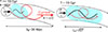 |
Fig. 1. Schematic view of the model. At early times, particles flow following the field lines and produce turbulence on small scales. At tage ≈ 10 Gyr, larger-scale turbulence is produced at greater distances from the source, and resonant scattering at high energies becomes efficient; particles are slowed down and reach a distance from the source that is comparable with their diffusive length, |
2.2. UHECR transport in the IGM
The nonlinear chain of phenomena that cause the excitation, growth, and saturation of the nonresonant instability as well as the transport of cosmic rays in the self-generated perturbations is extremely complex and poses a serious challenge not only from the computational point of view, but from the conceptual point of view as well. For instance, after a time τsat(E), particles with energy E are expected to be slowed down considerably, which means that their motion is no longer ballistic. Consequently, it might be argued that the previously proposed calculation of the current becomes inappropriate. As discussed by Blasi & Amato (2019), however, while self-confinement makes transport diffusive, the current in the region in which particles are confined remains unchanged at the lowest order: The current is conserved, but limited to a smaller region around the source. Particles are therefore confined and gradually leak outward if there is sufficient time.
Moreover, particles at a given energy E would also experience the turbulence that is produced by lower-energy particles on scales l ≪ RL(E) on timescales t < τsat(E). The transport of particles at a given energy is therefore expected to be affected by the self-generated turbulence on timescales that are shorter than the corresponding saturation time and to switch from ballistic to diffusive in a small-angle scattering regime (Subedi et al. 2017). For example, after one crossing time of the flux tube, τc = 2λB/c ≈ 0.2 Gyr λ30, particles with an energy Ec ≈ 10 PeV (Eq. (6)) have produced turbulence on a length scale lturb = Ec/eδB. With the diffusion coefficient expressed in Eq. (19) of Subedi et al. (2017), the diffusive length,  , is shorter than the correlation length of the magnetic field for particles with energy
  . The escape of particles with energies E ≲ Et is therefore inhibited on timescales shorter than τsat(E) by diffusion on small-scale perturbations that are produced by lower-energy particles that cross the flux tube.
Another complication arises from the fact that confinement causes the flux tube in which UHECRs are confined to become overpressured relative to the surrounding medium, so that the tube is expected to inflate a bubble that expands at roughly the Alfvén speed (Schroer et al. 2021, 2022). Because this speed is relatively low compared to the drift velocity of UHECRs due to diffusion, we neglected this phenomenon as well, although it might become important in the lower-energy region, in which transport is dominated by advection.
This scenario is highly conceptually complex. We therefore treated the escape of UHECRs from the source vicinity in a very simple but physically motivated way: The spectrum of the escaping particles is the same as that injected by the source for energies for which the escape time is shorter than tage, and it vanishes otherwise. We defined the escape time from the near-source region as follows:
 (11)
(11)
where  and
and  are the advective and diffusive timescale, respectively. These timescales are shown in Fig. 2a for λB = 30 Mpc, tage = 10 Gyr, and for different values of the source luminosity.
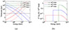 |
Fig. 2. Panel a: Relevant timescales for ℒp = 1043 erg/s (dashed), 1044 erg/s (solid), and 1045 erg/s (dotted). The vertical line shows the critical energy defined by RL(E) = R. Panel b: Cosmic-ray injection (Eq. (16)) for ℒp = 1043 erg/s (red), 1044 erg/s (blue), and 1045 erg/s (green). |
Although the diffusion coefficient is expected to be Bohm-like (Eq. (9)), the time required for the saturation of the nonresonant instability, τsat(E), at a sufficiently high energy exceeds tage. In this case, there will not be enough time for the generation of power on the resonant scale. Consequently, these particles undergo small pitch-angle scattering with a typical diffusion coefficient D(E)∝E2 (Subedi et al. 2017). As previously discussed, this behavior is expected to affect the particle transport at a given energy on timescales shorter than the corresponding saturation time, which instead marks the onset of Bohm diffusion, that is, resonant scattering on the turbulence. To account for this effect, we write the diffusion coefficient in the following generalized form:
![Mathematical equation: $$ \begin{aligned} D = \frac{c}{3} \left(\frac{E_c}{e \delta B}\right) \left[ \left(\frac{E}{E_c}\right) + \left(\frac{E}{E_c}\right)^2 \right], \end{aligned} $$](/articles/aa/full_html/2026/03/aa56040-25/aa56040-25-eq23.gif) (12)
(12)
where Ec is defined by the condition τsat(E) = tage. Depending on specific parameters, Ec is in the range ≈(0.1–1) EeV.
Moreover, when the particle energy becomes high enough for the gyration radius to exceed the size R of the source, the effective cross section of the flux tube increases as E2, and it becomes much harder to excite the nonresonant instability. This occurs when E ≳ ER, where ER ≃ eB0R ≃ EeV BnGRMpc. Lower-energy particles are initially assumed to move roughly along the ordered magnetic field, while some level of perpendicular diffusion is expected after substantial magnetic field amplification. We did not consider this phenomenon here. Finally, for particles that are not magnetized on a scale λB, namely when E ≳ EM with EM = eB0λB ≃ 30 EeV BnGλ30, the escape of the particles is quasi-ballistic and the effect of self-generation does not take place. When the preexisting magnetic field is ≈1 nG, this is not important because the energy range in which this occurs is close to or even in excess of the maximum energy of the protons that is compatible with the measured mass composition, namely a few EeV. For smaller strengths of the IGMF and when the coherence scale λB is much smaller than 10 Mpc, however, this becomes a serious concern because the particle propagation in the range ≲1 EeV becomes ballistic and the low-energy suppression disappears. To be on the safe side, the model discussed here therefore required the IGMF to be in the ≲nG range, with λB ≳ 10 Mpc, for the nonresonant instability to be of phenomenological relevance in the EeV energy range.
When these conditions are satisfied, the requirement that the instability is excited (Eq. (5)) translates into a minimum source luminosity in the form of cosmic rays,
 (13)
(13)
The Alfvén speed in the amplified field increases with the amplified magnetic field, which typically occurs when the source luminosity is higher. This increase would reduce the advection time, which might eventually become too short in the EeV range to guarantee CR confinement. The condition that the advection time exceeds the source age, VAtage ≳ λB, sets an upper limit on the source luminosity for which the considerations we discussed apply,
 (14)
(14)
For typical values of the parameters, this upper limit does not pose a severe concern for the applicability of our calculations. At the same time, the plasma is also pushed by the cosmic-ray pressure in the radial direction, and a low-density bubble is expected to expand at the same velocity (Schroer et al. 2021, 2022). An expansion over distances that are comparable with the source radial size is only expected for sources with power ℒp ≳ 1045 erg/s RMpc4, however.
When the source luminosity is within the range that is bounded by the values set by Eqs. (13) and (14), cosmic-ray confinement near the source occurs when the diffusion time exceeds the age of the source. This phenomenon results in a cutoff in the spectrum of UHECRs that are released into the IGM at energies below
 (15)
(15)
Depending on the source parameters and the value of λB, the condition τdiff(E) > tage is satisfied in the Bohm regime (EDBohm) or in the small-angle scattering regime (EDsas).
The estimate in Eq. (15) refers to the escape time evaluated at tage. The escape time of particles with an energy E ≳ ED is therefore shorter than the age of the source, even in the strongest turbulence that is produced within a timescale tage. Conversely, when we only consider the turbulence produced within one crossing time of the flux tube, the condition τesc(E) > tage is met at  . The total flux that escapes the confinement region is therefore expected to increase by a factor tage/τc in between the energy range Et ≲ E ≲ ED. It is highly complex to model the exact shape of this flux suppression, and this cannot be achieved in the context of the simple model presented here. We tried to adopt different prescriptions and verified that the conclusions are affected only quantitatively, but not qualitatively. We therefore adopted a simple but effective approach that captures the essential physics of the problem. In this context, we modeled the released spectrum of the source as
![Mathematical equation: $$ \begin{aligned} Q_{\mathrm{src}}(E,\mathcal{L} _{\rm p}) = q(E) \mathcal{H} \left[t_{\mathrm{age}} - \tau _{\mathrm{esc}}(E,\mathcal{L} _{\rm p}) \right], \end{aligned} $$](/articles/aa/full_html/2026/03/aa56040-25/aa56040-25-eq28.gif) (16)
(16)
where  , and the Heaviside function ℋ ensures that particles with escape times that exceed the age of the source remain confined within the source. Our modeling of the diffusion coefficient ensured that the condition τesc(E) = tage was met in the energy range Et ≲ E ≲ ED. The shape of the spectrum of escaping particles from the near-source region is shown in Fig. 2b for three values of the source luminosity, normalized to Emin = 1 GeV, and for our reference values of the environmental parameters, R = 1 Mpc, λB = 30 Mpc, B0 = 1 nG, and Emax = 3 EeV.
3. Results
3.1. Emissivity from a population of nonidentical sources
As discussed in the previous section, the spectrum of a source that is actually released into the IGM depends in a nonlinear way upon the source luminosity. Therefore, it is interesting to explore what happens when a luminosity function Φ(ℒp, z) is assumed for the putative source population. The case of identical sources with a single value of the luminosity, usually adopted in the literature on the origin of UHECRs for simplicity (see, e.g., Abdul Halim et al. 2023), can be recovered by restricting the luminosity function to a narrow range.
The emissivity in the form of protons as a function of energy at a given redshift can easily be calculated as
 (17)
(17)
where ℒlow and ℒhigh identify the minimum and maximum luminosity for which the luminosity function applies.
The simplest choice of a luminosity function, useful to clarify some points, is a power-law distribution,
 (18)
(18)
where V is the comoving volume, and A is a normalization constant with units of Mpc−3 erg−1 s.
The emissivity in the form of protons, given a power-law luminosity function, is shown in Fig. 3. The results for β = 1 are presented in the left panel for four different values of ℒhigh, as indicated. For β < 2, the emissivity at a given energy is dominated by the luminosity region near ℒhigh, and we therefore only changed the value of ℒhigh in the left panel. The suppression of the flux of protons that are injected at low energies is easily identifiable and is due to the self-confinement of UHECR near the sources. The suppression is not as sharp as that in Fig. 2 as a result of the convolution of different source luminosities. For β < 2, it can easily be shown that the energy dependence of the emissivity for self-confined particles is approximately 𝒬(E)∝E−2 + 4(2 − β)/3. The factor 4/3 derives from the proportionality between the cutoff energy and the source luminosity when the cutoff condition is met in the small-angle scattering regime, L ∝ E4/3; when the cutoff condition is satisfied in the Bohm regime, the proportionality between the cutoff energy and the source luminosity increases to L ∝ E2. This mimics a source spectrum that is harder than the canonical E−2, although this shape does not directly relate to the acceleration process, as discussed above. The drop in the emissivity for energies ≳3 EeV is due to a cutoff in the source spectrum at this energy, which is required to fit the Auger data, as was found in previous phenomenological descriptions (see, e.g., Aloisio & Berezinsky 2004; Abdul Halim et al. 2023). The curve corresponding to ℒhigh = 1048 erg/s shows a plateau at low energies (no suppression). This case highlights the role of advection: For high source luminosities, the CR current is so intense that the diffusion coefficient becomes very small and causes particles to escape due to advection with the self-generated perturbations. This case is only shown to illustrate the role of advection, but sources with this high CR luminosity might imply a possibly unrealistic total luminosity of the sources, at least when averaged over a time tage ≈ 10 Gyr.
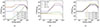 |
Fig. 3. Proton emissivity calculated from Eq. (17), considering a simple power-law luminosity function. Panel a: Different choices of ℒhigh, with β = 1 and ℒlow = 1040 erg/s. Panel b: Different choices of β, with ℒlow = 1040 erg/s and ℒhigh = 1044 erg/s. Panel c: Different choices of ℒlow, with β = 1 and ℒhigh = 1044 erg/s. |
In the central panel of Fig. 3, we present the emissivity for ℒlow = 1040 erg/s and ℒhigh = 1044 erg/s, with four values of β. For β = 1, the flux is clearly suppressed for E ≲ 0.6 EeV, as discussed previously. In the case of β = 2.5(≥2), the main contribution to the emissivity is provided by low-luminosity sources, for which the self-confinement is limited to lower-energy CRs, as illustrated by the green curve in the central panel of Fig. 3. Given the low value of ℒlow < ℒmin, the spectrum at very low energy (≲30 PeV) is dominated by sources that are unable to produce the NRSI, and it resembles the accelerated spectrum.
Finally, we show in the right panel of Fig. 3 the emissivity in the form of protons for β = 1 and different values of ℒlow, while ℒhigh is fixed to the value of 1044 erg/s. As in the previous cases, the high-energy suppression arises because we adopted an exponential cutoff at 3 EeV. Higher values of ℒlow result in a more pronounced suppression of the emissivity at higher energies compared to lower ℒlow values. As a consequence, the region in which the emissivity hardens due to the convolution with the luminosity function extends to a narrower energy region when ℒlow increases. Nonetheless, in all scenarios, the effect of self-confinement together with the convolution with a luminosity function causes a mimicking of a hard injection spectrum. This is again unrelated to the intrinsic spectrum of accelerated particles.
The case of a simple power-law luminosity function, as illustrated above, provides useful insights into the expected effects: Luminous sources cause a self-confinement of UHECRs that extends to higher energies, and the convolution with a luminosity function for β < 2 leads to a hardening below the energy for which confinement is caused by sources with a luminosity of about ℒhigh. In this energy range, the spectrum behaves as 𝒬(E)∝E−2 + 4(2 − β)/3. For β > 2, the confinement is dominated by the sources with the lowest luminosity.
This case might be sufficient to support the physical picture in which we are interested. Because in many cases, however, the luminosity function is modeled as a broken power law, for instance, in the cases of active galactic nuclei (AGN) and starburst galaxies as sources or astrophysical objects that host the sources, we briefly discuss this scenario using the following functional form for the luminosity function:
![Mathematical equation: $$ \begin{aligned} \Phi (\mathcal{L} _{\rm p},z) = \frac{dN}{d\mathcal{L} _{\rm p} dV} = \frac{A e(z)}{\log (10) \mathcal{L} _{\rm p}} \left[ \left( \frac{\mathcal{L} _{\rm p}}{\mathcal{L} _*} \right)^{\gamma _1} + \left( \frac{\mathcal{L} _{\rm p}}{\mathcal{L} _*} \right)^{\gamma _2} \right]^{-1}, \end{aligned} $$](/articles/aa/full_html/2026/03/aa56040-25/aa56040-25-eq32.gif) (19)
(19)
where V is the comoving volume, γi are the slopes characterizing the low- and high-luminosity behavior, L* is a break luminosity, and A is a normalization constant. The term e(z) can be chosen to model the redshift evolution of the luminosity function, which varies with the source population. For simplicity and for the sole purpose of illustrating the physical results, we adopted a constant redshift evolution e(z) = 1 up to zmax = 3. A more detailed review of the luminosity distribution modeling for galaxies and AGN-like objects can be found in Fotopoulou et al. (2016). As in the previous case, the emissivity in the form of protons was computed using Eq. (17). We show our results in Fig. 4 for different choices of the parameters that define the luminosity function.
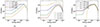 |
Fig. 4. Proton emissivity calculated from Eq. (17), considering a broken power-law luminosity function (Eq. (19)) with γ2 = 2.5. Panel a: Different positioning of ℒ*; the low luminosity index is γ1 = 0.5. Panel b: Different low-luminosity behavior; the positioning of the break is fixed at ℒ* = 1044 erg/s. Panel c: Different choices of ℒlow; the position of the break is ℒ* = 1044 erg/s and the slope is γ1 = 0.5. |
Given the wide variety of possible choices of the values of the parameters, we tried to find guidance in the luminosity function for some sources, such as that of AGN-like sources, for which values of γ1 ≲ 1 and γ2 ≳ 2 are typically fit in the X-ray (Ajello et al. 2009; Burlon et al. 2011) and γ-ray (Ajello et al. 2012; Qu et al. 2019) bands. Based on the results found for a power-law luminosity function, most results of physical relevance are clearly determined by the choice of γ1 and ℒ*. Therefore, we fixed γ2 = 2.5 and briefly comment on the dependence of the results on the other parameters. Again, we used our findings in the power-law case as guidance: Most of our previous conclusions still hold when the role of ℒhigh is now played by ℒ* and the role of β is played by γ1 < 1. In this way, the interpretation of the three panels in Fig. 4 is straightforward. As in the previous case, the high-energy exponential drop in the emissivity is due to the assumed maximum energy of protons in the accelerator.
3.2. Diffuse proton flux
We focused on the spectrum of protons at the Earth, when the source spectrum is computed by accounting for self-confinement, as discussed above. The propagated flux of protons at z = 0 was calculated following Berezinsky et al. (2006) and reads
 (20)
(20)
where  , and the Jacobian
  is determined by the energy losses of the protons during transport. We included pair production and photo-pion production on the cosmic microwave background (CMB) radiation field as channels of energy losses, and we computed the corresponding energy loss rates as functions of energy and redshift by interpolating numerical tables generated using the latest release of the code SimProp (Aloisio et al. 2017). The adopted cosmology is the Planck ΛCDM model, with h = 0.67, Ωm = 0.32, and ΩΛ = 0.68 (Planck Collaboration XIII 2016).
3.3. Diffuse neutrinos from UHECR sources
In the standard scenario, UHECRs are promptly injected by sources into the IGM and propagate over cosmological distances. During their journey, interactions with background radiation fields generate a cosmogenic neutrino flux, which is directly tied to the flux of protons that reach the Earth.
In contrast, the scenario we discussed here (like other scenarios involving near-source confinement; Unger et al. 2015; Muzio et al. 2022) introduces an additional contribution to the diffuse neutrino background. This contribution arises from UHECRs that are unable to escape their near-source regions. In our framework, protons that are confined within the source environment cannot propagate into the IGM, but might still produce neutrinos via photo-pion production.
The relatively low maximum energies allowed by current mass-composition measurements mean that most of these interactions occur with the extragalactic background light (EBL) and not with the CMB alone. For the EBL, we adopted the most recent determination, which was provided by Saldana-Lopez et al. (2021). While the local EBL near sources might in principle exceed the average EBL, we neglected this effect here because it strongly depends on the specific type of source under consideration.
We describe the calculation of the neutrino flux produced by confined UHECRs, Jνconf, below and compare it to the purely cosmogenic neutrino flux, Jνcosmo, which arises from UHECRs that successfully escape from the near-source regions.
In the calculations of the effect of photo-pion production, we made use of the parameterization of the differential cross section described by Kelner & Aharonian (2010), which is obtained by fitting the energy distribution of the photo-pion interactions resulting from particle physics simulations performed with the code SOPHIA (Mücke et al. 2000). The energy distribution of the outgoing neutrinos was parameterized in terms of the energy fraction of the impinging proton taken by the emitted neutrino, x = Eν/Ep. Based on the same formalism as adopted by Kelner & Aharonian (2010), the number of neutrinos produced per unit time and energy in the entire volume defined by the flux tube around a source is given by
 (21)
(21)
where Np(E, t) is the number of protons with energy E that are confined within the flux tube at the time t, and ℛ(Ep, Eν, z) is the production rate of neutrinos with energy Eν from protons with energy Ep that interact with the background photons at redshift z. The production rate is defined using the parameterized cross-section as
 (22)
(22)
where ϵth(Ep) identifies the threshold energy for the photo-pion interaction. To estimate the number of protons that are confined within the flux tube, we considered a continuous injection of protons from the source at a rate q(E) and continuous escape from the flux tube at a rate defined by Eq. (11),
 (23)
(23)
The solution at t = tage holds
![Mathematical equation: $$ \begin{aligned} N_p(E_p,t_{\rm age}) = q(E_p) \tau _{\rm esc}(E_p) \left[ 1 - e^{-\frac{t_{\rm age}}{\tau _{\rm esc}(E_p)}} \right], \end{aligned} $$](/articles/aa/full_html/2026/03/aa56040-25/aa56040-25-eq39.gif) (24)
(24)
which depends nontrivially on the source luminosity through the proton escape time. The cosmological neutrino emissivity from confined protons was obtained by summing over the contribution of all the sources,
 (25)
(25)
Finally, the neutrino flux at Earth was obtained by solving the cosmological transport equation,
 (26)
(26)
On the other hand, the flux of cosmogenic neutrinos is generated by unconfined protons that propagate over cosmological distances. The spectral proton density at arbitrary redshift was determined in a way similar to that of Berezinsky et al. (2006),
 (27)
(27)
Hence, the cosmogenic neutrino emissivity reads
 (28)
(28)
and the diffuse cosmogenic neutrino flux at Earth was calculated as in Eq. (26),
 (29)
(29)
3.4. Comparison with observations
The flux of CR protons from sources that are distributed with a luminosity function is shown in Fig. 5, together with the all-particle spectrum measured by Auger (Abreu et al. 2021, 2020) and the proton spectrum obtained by adopting the mass fraction computed in Aab et al. (2016, Aab et al. (2014a,b) using EPOS-LHC (Pierog et al. 2015). The parameters defining the luminosity function for all the tested cases are listed in Table 1.
List of parameters.
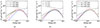 |
Fig. 5. Cosmic-ray intensity at Earth. Panel a: Different positioning of ℒ*, with γ1 = 0.5. Panel b: Different slope, with the positioning of the break fixed at ℒ* = 1044 erg/s. Panel c: Different choices of ℒlow, with ℒ* = 1044 erg/s and γ1 = 0.5. γ2 = 2.5 in all the cases. The all-particle spectrum (Abreu et al. 2021; Aab et al. 2020) measured by Auger and the proton fraction (Aab et al. 2014a,b, 2016) inferred through the EPOS-LHC hadronic interaction model (Pierog et al. 2015) are shown with black squares and red circles, respectively. As a comparison, the same result is shown for an injection Qsrc(E)∝E−2 (dashed black). |
The three panels refer to the relevant cases illustrated in Fig. 4, and the normalization constant of the LF was chosen to avoid overshooting the proton spectrum measured by the Auger in the ankle region. As can be inferred from the comparison with an injection spectrum of E−2 (dashed black), the confinement mechanism we proposed is not necessary to explain the fraction of protons around 1018 eV, whereas it might be relevant for the cosmic-ray spectrum above the ankle, where the inferred mass composition is increasingly heavier and the required spectral index at the escape from the source is unusually hard (Abdul Halim et al. 2023). The possibility that the sources of the highest-energy cosmic rays also accelerate protons, although in a smaller fraction than heavier nuclei, cannot be excluded, however (Muzio et al. 2024). Moreover, in this scenario, interactions within the confinement region lead to the production of secondary protons (Unger et al. 2015).
We then used the proton flux constrained by Auger data to derive an estimate of the contribution to the diffuse neutrino flux of these sources, provided the proposed mechanism is in place. In doing so, we assumed that the maximum proton content allowed for the UHECR population that dominates above the ankle is restricted by the proton fraction measured by Auger, as in Fig. 5.
The two contributions, Jνcosmo and Jνconf, are shown in Fig. 6 for the same cases as illustrated in Fig. 5, with the same choice of the normalization constant. The neutrino flux produced by confined protons exceeds the cosmogenic flux in the (1–100) PeV energy range. The total neutrino flux remains compatible with the upper limits posed by the Ice Cube experiment (Kopper 2017; Abbasi et al. 2025) even for the maximum choice about the proton flux, however, as discussed before.
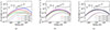 |
Fig. 6. Total diffuse neutrino flux at Earth (solid) from confined (dashed lines) and diffused protons (dotted lines). Panel a: Different positioning of ℒ*, with γ1 = 0.5. Panel b: Different slope, with the positioning of the break fixed at ℒ* = 1044 erg/s. Panel c: Different choices of ℒlow, with ℒ* = 1044 erg/s and γ1 = 0.5. γ2 = 2.5 in all the cases. Measurements (black dots) and upper limits (black line and arrows) obtained by the Ice Cube Observatory Aartsen et al. (2013), Kopper (2017), Abbasi et al. (2025) are shown for comparison. |
A detailed study and comparison with the spectrum and mass composition as measured by Auger, including the nuclei and the related interactions inside the confinement environment, will be fully addressed in a forthcoming work.
4. Discussion and conclusions
The Auger data on the UHECR spectrum and mass composition unequivocally indicate that the dominant population of sources above the ankle (Abdul Halim et al. 2023) must inject a spectrum with a remarkably hard shape and a maximum energy in the range of a few EeV. The term “sources” here refers to astrophysical objects that might either host the real accelerators or act as storage environments for cosmic rays. This distinction is well illustrated by galaxy clusters, which have long been recognized as natural reservoirs for cosmic rays over cosmological timescales (Berezinsky et al. 1997; Ensslin et al. 1997). Within these clusters, cosmic rays can be accelerated either by shocks in the intracluster medium or by individual galaxies. For cosmic rays with energies ≲PeV, the confinement time often exceeds the age of the Universe, which leads to a natural low-energy suppression that effectively hardens the spectrum. The Auger data suggest that this hardening likely occurs in the ≲EeV energy range.
This spectral hardening might also result from pronounced confinement processes similar to those inferred in galaxy clusters (Berezinsky et al. 1997; Ensslin et al. 1997). For instance, a combination of confinement and energy losses in specific sources (Unger et al. 2015; Muzio et al. 2022) or the magnetic horizon effect, according to which strong extragalactic magnetic fields create a low-energy cutoff (Aloisio & Berezinsky 2004; Mollerach & Roulet 2013; Abdul Halim et al. 2024) can mimic this phenomenon. The latter explanation requires relatively large magnetic fields, however, which might be only marginally consistent with observational constraints, such as Faraday rotation measures, if these fields are ubiquitous.
We proposed an alternative mechanism for this hardening: Self-confinement driven by the excitation of plasma instabilities near powerful UHECR sources. When the energy density of escaping UHECRs exceeds the background magnetic field energy density, self-generated turbulence can significantly alter particle transport. We extended previous studies (Blasi et al. 2015) by exploring the environmental conditions under which self-confinement occurs at EeV energies. We calculated the resulting UHECR proton spectrum and diffuse neutrino flux in this framework.
Our results confirm that the scattering of UHECRs on self-generated magnetic perturbations leads to confinement timescales that exceed the source age for particles with ≲EeV energies. This effect imprints a low-energy suppression in the UHECR spectrum at Earth, affected by the luminosity function of the sources.
The mechanism is particularly efficient when the source luminosity is ≈1044 erg/s and when the preexisting IGMF is in the nG range, within a region of ≈30 Mpc around the source. Notably, the nonresonant instability might still grow for lower values of B0 when particles down to ≈PeV contribute to the current (see Eq. (7)). These conditions might naturally arise in environments such as galaxy clusters, where the interplay between confinement and turbulence is prominent. Depending on the magnetic field, very low-energy particles (≲ PeV) might also contribute to the current and produce the instability in the IGM. The distance from the source they might explore within the age of the Universe, however, is typically shorter than the source size because their diffusive length is short. These particles also drive the stronger pressure gradient on the background plasma. We stress the relevance of considering the source not as the accelerator, but the astrophysical object that hosts it. For instance, for galaxy clusters as the sources that host the accelerators, it is known that particles up to some energy, typically in the 100–1000 TeV range, might be diffusively confined in the cluster volume due to preexisting MHD turbulence (Berezinsky et al. 1997; Völk et al. 1996).
Conversely, particles with higher energy (≳10 PeV) are likely able to escape from the source region and produce perturbations in the near source region, as discussed here, and in doing so, they are expected to be self-confined.
Resonant diffusion requires a saturation time to set on, but on timescales t < τsat(E), particle transport is affected by small-angle scattering on the turbulence produced by lower-energy particles. Consequently, particle escape at energy E is reduced on timescales shorter than τsat(E).
We stress again, given the importance of the point, that most potential UHECR accelerators, such as AGNs (Pimbblet et al. 2012) or sources in starburst galaxies (Paccagnella et al. 2017), are indeed expected to reside within galaxy clusters. These regions are seen to be magnetized and are an integral part of the filamentary structure of the large-scale Universe (Vernstrom et al. 2021; Carretti et al. 2022). Cosmic rays are well confined inside these structures, so that only CRs with E ≳ 100 − 1000 TeV can escape (Berezinsky et al. 1997; Völk et al. 1996).
As discussed in Sect. 2.1, an original magnetic field strength in the nG range is needed for the NRSI to be of phenomenological relevance in the EeV energy range. When only high-energy particles leak from the source, as is the case for galaxy clusters, thermal effects that slow down (Eq. (8)) or inhibit (Eq. (7)) the instability are irrelevant.
We calculated the UHECR proton flux from a cosmological population of sources with a typical luminosity function and compared our predictions with the Auger proton fraction (Abreu et al. 2021; Aab et al. 2020, 2014a,b, 2016), interpreted using the EPOS-LHC hadronic interaction model (Pierog et al. 2015). Our results predict an excess of neutrino production in the near-source regions due to self-confinement of UHECRs with E ≲ 1 EeV, compared to the cosmogenic neutrino flux from intergalactic space. The total neutrino flux remains consistent with current observational upper limits, however (Kopper 2017; Abbasi et al. 2025).
Finally, our model predicts that powerful UHECR sources are surrounded by regions that extend to tens of megaparsec, with turbulent magnetic fields that reach nG levels because the nonresonant instability is saturated. Observations of X-ray and radio emissions already suggest that magnetized structures connect galaxy clusters (Vernstrom et al. 2021), with average magnetic fields of 30–50 nG on scales ≳3 Mpc. Faraday rotation measures, which are sensitive to the mean magnetic field direction, impose upper limits on large-scale fields at the level of a few nG (O’Sullivan et al. 2020). These limits scale linearly with the assumed electron density, however, which implies that magnetic fields in overdense regions, such as filaments, might be larger by at least an order of magnitude. An original magnetic field strength B0 ≳ nG, needed for self-confinement to affect UHECRs at the EeV energy scale, is compatible with actual observations.
The effect of amplified magnetic fields on Faraday rotation remains challenging to quantify because it depends on the source luminosity function. The average effect on the rotation measure can be estimated through the product of the average amplified magnetic field, the filling factor, and the average electron density, ⟨Rf⟩≈f1/2ne⟨δB⟩ (Amaral et al. 2021), where ⟨δB⟩ is the average amplified field strength weighted by the source luminosity function, ne is the mean electron density, and f is the filling factor, determined by the product of the source density and the volume of a single flux tube.
Assuming the same electron density as in Amaral et al. (2021), ne ≃ 10−5 cm−3, we estimate ⟨Rf⟩≈10−9 μG cm−3, which is lower by roughly an order of magnitude than the limits of the residual rotation measure limits reported by Amaral et al. (2021). The values of the averaged amplified field, filling factor, and ⟨Rf⟩ are reported in Table 1 for all cases we tested.
Acknowledgments
This work was partially funded by the European Union – NextGenerationEU under the MUR National Innovation Ecosystem grant ECS00000041 – VITALITY/ASTRA – CUP D13C21000430001. The work of PB was also partially funded by the European Union – Next Generation EU, through PRIN-MUR 2022TJW4EJ.
References
- Aab, A., Abreu, P., Aglietta, M., et al. 2014a, Phys. Rev. D, 90, 122006 [NASA ADS] [CrossRef] [Google Scholar]
- Aab, A., Abreu, P., Aglietta, M., et al. 2014b, Phys. Rev. D, 90, 122005 [NASA ADS] [CrossRef] [Google Scholar]
- Aab, A., Abreu, P., Aglietta, M., et al. 2016, Phys. Lett. B, 762, 288 [NASA ADS] [CrossRef] [Google Scholar]
- Aab, A., Abreu, P., Aglietta, M., et al. 2017, JCAP, 2017, 038 [CrossRef] [Google Scholar]
- Aab, A., Abreu, P., Aglietta, M., et al. 2020, Phys. Rev. D, 102, 062005 [NASA ADS] [CrossRef] [Google Scholar]
- Aartsen, M. G., Abbasi, R., Abdou, Y., et al. 2013, Phys. Rev. Lett., 111, 021103 [Google Scholar]
- Aartsen, M. G., Ackermann, M., Adams, J., et al. 2019, Phys. Rev. D, 100, 082002 [Google Scholar]
- Abbasi, R., Ackermann, M., Adams, J., et al. 2025, Phys. Rev. Lett., 135, 031001 [Google Scholar]
- Abdul Halim, A., Abreu, P., Aglietta, M., et al. 2023, JCAP, 2023, 024 [CrossRef] [Google Scholar]
- Abdul Halim, A., Abreu, P., Aglietta, M., et al. 2024, JCAP, 2024, 094 [Google Scholar]
- Abreu, P., Aglietta, M., Albury, J. M., et al. 2021, EPJ C, 81, 1 [Google Scholar]
- Ajello, M., Costamante, L., Sambruna, R. M., et al. 2009, ApJ, 699, 603 [NASA ADS] [CrossRef] [Google Scholar]
- Ajello, M., Shaw, M. S., Romani, R. W., et al. 2012, ApJ, 751, 108 [NASA ADS] [CrossRef] [Google Scholar]
- Aloisio, R., & Berezinsky, V. 2004, ApJ, 612, 900 [NASA ADS] [CrossRef] [Google Scholar]
- Aloisio, R., Boncioli, D., di Matteo, A., et al. 2017, JCAP, 2017, 009 [CrossRef] [Google Scholar]
- Amaral, A. D., Vernstrom, T., & Gaensler, B. M. 2021, MNRAS, 503, 2913 [NASA ADS] [CrossRef] [Google Scholar]
- Amato, E., & Blasi, P. 2009, MNRAS, 392, 1591 [Google Scholar]
- Arons, J. 2003, ApJ, 589, 871 [NASA ADS] [CrossRef] [Google Scholar]
- Asano, K., & Mészáros, P. 2016, Phys. Rev. D, 94, 023005 [Google Scholar]
- Bell, A. R. 2004, MNRAS, 353, 550 [Google Scholar]
- Bell, A. R., Schure, K. M., Reville, B., & Giacinti, G. 2013, MNRAS, 431, 415 [Google Scholar]
- Berezinsky, V. S., Blasi, P., & Ptuskin, V. S. 1997, ApJ, 487, 529 [NASA ADS] [CrossRef] [Google Scholar]
- Berezinsky, V., Gazizov, A., & Grigorieva, S. 2006, Phys. Rev. D, 74, 043005 [Google Scholar]
- Bergman, D. 2006, JPCS, 47, 154 [Google Scholar]
- Blandford, R., & Eichler, D. 1987, Phys. Rep., 154, 1 [Google Scholar]
- Blandford, R. D., & Ostriker, J. P. 1978, ApJ, 221, L29 [Google Scholar]
- Blasi, P., & Amato, E. 2019, Phys. Rev. Lett., 122, 051101 [CrossRef] [Google Scholar]
- Blasi, P., Epstein, R. I., & Olinto, A. V. 2000, ApJ, 533, L123 [NASA ADS] [CrossRef] [Google Scholar]
- Blasi, P., Amato, E., & D’Angelo, M. 2015, Phys. Rev. Lett., 115, 121101 [Google Scholar]
- Burlon, D., Ajello, M., Greiner, J., et al. 2011, ApJ, 728, 58 [Google Scholar]
- Carretti, E., O’Sullivan, S. P., Vacca, V., et al. 2022, MNRAS, 518, 2273 [NASA ADS] [CrossRef] [Google Scholar]
- Ensslin, T. A., Biermann, P. L., Kronberg, P. P., & Wu, X.-P. 1997, ApJ, 477, 560 [Google Scholar]
- Fotopoulou, S., Buchner, J., Georgantopoulos, I., et al. 2016, A&A, 587, A142 [NASA ADS] [CrossRef] [EDP Sciences] [Google Scholar]
- Kang, D. 2023, PoS, ICRC2023, 307 [Google Scholar]
- Kelner, S. R., & Aharonian, F. A. 2010, Phys. Rev. D, 82, 099901 [Google Scholar]
- Kopper, C. 2017, PoS, ICRC2017, 981 [Google Scholar]
- Kotera, K., Amato, E., & Blasi, P. 2015, JCAP, 2015, 026 [CrossRef] [Google Scholar]
- Mollerach, S., & Roulet, E. 2013, JCAP, 2013, 013 [CrossRef] [Google Scholar]
- Mücke, A., Engel, R., Rachen, J. P., Protheroe, R. J., & Stanev, T. 2000, Comput. Phys. Commun., 124, 290 [Google Scholar]
- Muzio, M. S., Farrar, G. R., & Unger, M. 2022, Phys. Rev. D, 105, 023022 [CrossRef] [Google Scholar]
- Muzio, M. S., Anchordoqui, L. A., & Unger, M. 2024, Phys. Rev. D, 109, 023006 [Google Scholar]
- O’Sullivan, S. P., Brüggen, M., Vazza, F., et al. 2020, MNRAS, 495, 2607 [Google Scholar]
- Paccagnella, A., Vulcani, B., Poggianti, B. M., et al. 2017, ApJ, 838, 148 [NASA ADS] [CrossRef] [Google Scholar]
- Pierog, T., Karpenko, I., Katzy, J. M. E. A., 2015, Phys. Rev. C, 92, 034906 [NASA ADS] [CrossRef] [Google Scholar]
- Pimbblet, K. A., Shabala, S. S., Haines, C. P., Fraser-McKelvie, A., & Floyd, D. J. E. 2012, MNRAS, 429, 1827 [Google Scholar]
- Planck Collaboration XIII. 2016, A&A, 594, A13 [NASA ADS] [CrossRef] [EDP Sciences] [Google Scholar]
- Qu, Y., Zeng, H., & Yan, D. 2019, MNRAS, 490, 758 [Google Scholar]
- Riquelme, M. A., & Spitkovsky, A. 2009, ApJ, 694, 626 [Google Scholar]
- Saldana-Lopez, A., Domínguez, A., Pérez-González, P. G., et al. 2021, MNRAS, 507, 5144 [CrossRef] [Google Scholar]
- Schroer, B., Pezzi, O., Caprioli, D., Haggerty, C., & Blasi, P. 2021, ApJ, 914, L13 [NASA ADS] [CrossRef] [Google Scholar]
- Schroer, B., Pezzi, O., Caprioli, D., Haggerty, C., & Blasi, P. 2022, MNRAS, 512, 233 [NASA ADS] [CrossRef] [Google Scholar]
- Shinozaki, K., & Teshima, M. 2004, Nucl. Phys. B Proc. Suppl., 136, 18 [Google Scholar]
- Sironi, L., Keshet, U., & Lemoine, M. 2015, SSR, 191, 519 [Google Scholar]
- Subedi, P., Sonsrettee, W., Blasi, P., et al. 2017, ApJ, 837, 140 [Google Scholar]
- Unger, M., Farrar, G. R., & Anchordoqui, L. A. 2015, Phys. Rev. D, 92, 123001 [CrossRef] [Google Scholar]
- Vernstrom, T., Heald, G., Vazza, F., et al. 2021, MNRAS, 505, 4178 [NASA ADS] [CrossRef] [Google Scholar]
- Völk, H. J., Aharonian, F. A., & Breitschwerdt, D. 1996, SSR, 75, 279 [Google Scholar]
- Zhang, H., Sironi, L., Giannios, D., & Petropoulou, M. 2023, ApJ, 956, L36 [NASA ADS] [CrossRef] [Google Scholar]
- Zweibel, E. G., & Everett, J. E. 2010, ApJ, 709, 1412 [NASA ADS] [CrossRef] [Google Scholar]
All Tables
All Figures
|
Fig. 1. Schematic view of the model. At early times, particles flow following the field lines and produce turbulence on small scales. At tage ≈ 10 Gyr, larger-scale turbulence is produced at greater distances from the source, and resonant scattering at high energies becomes efficient; particles are slowed down and reach a distance from the source that is comparable with their diffusive length, |
| In the text | |
|
Fig. 2. Panel a: Relevant timescales for ℒp = 1043 erg/s (dashed), 1044 erg/s (solid), and 1045 erg/s (dotted). The vertical line shows the critical energy defined by RL(E) = R. Panel b: Cosmic-ray injection (Eq. (16)) for ℒp = 1043 erg/s (red), 1044 erg/s (blue), and 1045 erg/s (green). |
| In the text | |
|
Fig. 3. Proton emissivity calculated from Eq. (17), considering a simple power-law luminosity function. Panel a: Different choices of ℒhigh, with β = 1 and ℒlow = 1040 erg/s. Panel b: Different choices of β, with ℒlow = 1040 erg/s and ℒhigh = 1044 erg/s. Panel c: Different choices of ℒlow, with β = 1 and ℒhigh = 1044 erg/s. |
| In the text | |
|
Fig. 4. Proton emissivity calculated from Eq. (17), considering a broken power-law luminosity function (Eq. (19)) with γ2 = 2.5. Panel a: Different positioning of ℒ*; the low luminosity index is γ1 = 0.5. Panel b: Different low-luminosity behavior; the positioning of the break is fixed at ℒ* = 1044 erg/s. Panel c: Different choices of ℒlow; the position of the break is ℒ* = 1044 erg/s and the slope is γ1 = 0.5. |
| In the text | |
|
Fig. 5. Cosmic-ray intensity at Earth. Panel a: Different positioning of ℒ*, with γ1 = 0.5. Panel b: Different slope, with the positioning of the break fixed at ℒ* = 1044 erg/s. Panel c: Different choices of ℒlow, with ℒ* = 1044 erg/s and γ1 = 0.5. γ2 = 2.5 in all the cases. The all-particle spectrum (Abreu et al. 2021; Aab et al. 2020) measured by Auger and the proton fraction (Aab et al. 2014a,b, 2016) inferred through the EPOS-LHC hadronic interaction model (Pierog et al. 2015) are shown with black squares and red circles, respectively. As a comparison, the same result is shown for an injection Qsrc(E)∝E−2 (dashed black). |
| In the text | |
|
Fig. 6. Total diffuse neutrino flux at Earth (solid) from confined (dashed lines) and diffused protons (dotted lines). Panel a: Different positioning of ℒ*, with γ1 = 0.5. Panel b: Different slope, with the positioning of the break fixed at ℒ* = 1044 erg/s. Panel c: Different choices of ℒlow, with ℒ* = 1044 erg/s and γ1 = 0.5. γ2 = 2.5 in all the cases. Measurements (black dots) and upper limits (black line and arrows) obtained by the Ice Cube Observatory Aartsen et al. (2013), Kopper (2017), Abbasi et al. (2025) are shown for comparison. |
| In the text | |
Current usage metrics show cumulative count of Article Views (full-text article views including HTML views, PDF and ePub downloads, according to the available data) and Abstracts Views on Vision4Press platform.
Data correspond to usage on the plateform after 2015. The current usage metrics is available 48-96 hours after online publication and is updated daily on week days.
Initial download of the metrics may take a while.