| Issue |
A&A
Volume 707, March 2026
|
|
|---|---|---|
| Article Number | A335 | |
| Number of page(s) | 10 | |
| Section | Extragalactic astronomy | |
| DOI | https://doi.org/10.1051/0004-6361/202556269 | |
| Published online | 18 March 2026 | |
Chromatic activity window of periodic fast radio bursts: FRB 20121102A and FRB 20180916B
1
Department of Astronomy, Universidad de Chile, Camino El Observatorio, 1515 Las Condes, Santiago, Chile
2
Centre of Astro-Engineering, Pontificia Universidad Católica de Chile, Av. Vicuña Mackenna 4860, Santiago, Chile
3
Department of Electrical Engineering, Pontificia Universidad Católica de Chile, Av. Vicuña Mackenna 4860, Santiago, Chile
4
Joint ALMA Observatory, Alonso de Córdova 3107, Vitacura, Santiago, Chile
5
European Southern Observatory, Alonso de Córdova 3107, Vitacura Casilla 19001 Santiago de Chile, Chile
6
Max-Planck-Institut für Radioastronomie, Auf dem Hügel 69, D-53121 Bonn, Germany
7
Department of Electrical Engineering, Universidad de Chile, Av. Tupper 2007, Santiago, Chile
8
Instituto de Astrofísica, Facultad de Física, Pontificia Universidad Católica de Chile, Casilla 306, Santiago 22, Chile
★ Corresponding author: This email address is being protected from spambots. You need JavaScript enabled to view it.
Received:
4
July
2025
Accepted:
4
January
2026
Abstract
Context. Two fast radio bursts, FRB 20121102A and FRB 20180916B, show periodic activity with cycles of 159.3 and 16.33 days, respectively. These cycles consist of active and inactive windows, with the peak activity centred within the active phase. For FRB 20180916B, studies reported a frequency-dependent or chromatic behaviour, for which the activity window starts earlier and becomes narrower at higher frequencies. The activity across frequencies is typically modelled with a power law.
Aims. We developed a simple model that combines the phase and frequency dependence of the activity windows of FRB 20121102A and FRB 20180916B. Our goal was to perform a chromaticity study for FRB 20121102A that incorporates model improvements to account for the cyclic nature of its activity window and to compare the chromatic behaviour of the two periodic FRBs.
Methods. We standardised the detections from the 425 observing epochs for FRB 20121102A and the 214 epochs for FRB 20180916B to account for differences in the radio telescope sensitivity. To the normalised detection-rate phase distribution, we fitted a von Mises distribution and extracted the peak activity phase and activity width. These quantities as a function of frequency were then modelled as power laws to construct the chromatic model.
Results. The activity window starts earlier at higher frequencies for the two sources. The activity window of FRB 20121102A broadens at higher frequencies, however, and that of FRB 20180916B broadens at lower frequencies. Interestingly, it appears to remain active during at least 80% of the cycle at C band.
Conclusions. The observed chromatic behaviour of FRB 20180916B is consistent with previous findings. For FRB 20121102A, a chromaticity in its activity window is also seen, but the source appears to be active for longer at higher frequencies, which is different from the behaviour of FRB 20180916B.
Key words: methods: data analysis / radio continuum: general
© The Authors 2026
 Open Access article, published by EDP Sciences, under the terms of the Creative Commons Attribution License (https://creativecommons.org/licenses/by/4.0), which permits unrestricted use, distribution, and reproduction in any medium, provided the original work is properly cited.
This article is published in open access under the Subscribe to Open model. This email address is being protected from spambots. You need JavaScript enabled to view it. to support open access publication.
1. Introduction
First discovered by Lorimer et al. (2007), fast radio bursts (FRBs) are an astronomical phenomenon that consists of exceptionally bright (1036–1041 erg, Zhang 2018; Locatelli et al. 2019) coherent radio pulses with durations from micro- to milliseconds (Zhang 2023). In addition to the Galactic magnetar SGR 1935+2154, which was observed to emit millisecond radio pulses (CHIME/FRB Collaboration 2020b), most FRBs are known to have an extragalactic origin. This is supported by their observed dispersive delay contribution, which is consistent with localised host galaxies (Chatterjee et al. 2017; Marcote et al. 2022; Tendulkar et al. 2017; Petroff et al. 2022; Cassanelli et al. 2024). These delays are quantified through the dispersion measure (DM; in pc cm−3) relation,
 (1)
(1)
which refers to the number density of electrons (ne) integrated along the path travelled by the photons from the source to the observer. The observed dispersive delay (Δt) is expressed as:
 (2)
(2)
where kDM = 1/(2.41 × 10−4) pc−1cm−1 MHz2s, νlow and νhigh are the lower and higher passband frequencies (MHz) (Lorimer & Kramer 2004).
The discovery of the first repeating FRB, FRB 20121102A (Spitler et al. 2016), led to the classification of FRBs into two categories: repeaters and one-offs. To date, around ∼800 FRB sources have been reported, and only 8.6% were identified as repeaters (Xu et al. 2023). According to Law et al. (2022), as few as 1% are highly active repeaters. This subsample corresponds to the sources with a high potential for multi-wavelength follow-up and long-term monitoring.
Three objects are reported to have periodic activity, FRB 20121102A (Rajwade et al. 2020; Cruces et al. 2021; Braga et al. 2025), FRB 20180916B (CHIME/FRB Collaboration 2020a), and FRB 20240209A (Pal 2025), which have alternating on- and off-activity cycles. The period of FRB 20121102A is approximately 159 days, with an active phase lasting 53% of this cycle (Braga et al. 2025). FRB 20180916B displays a ∼16-day periodicity and an on-phase of about 31% (CHIME/FRB Collaboration 2020a; Bethapudi et al. 2023). Most recently, it was reported that FRB 20240209A follows a ∼126–day cycle, with an activity window covering nearly 70% of the period (Pal 2025). These cases might indicate that multiple repeating FRBs have an active window that repeats at different period lengths, and some are significantly larger. This might explain the lack of a detected periodicity for some repeating FRBs.
As noted by Pastor-Marazuela et al. (2021), the activity window of FRBs seems to depend on the frequency. These authors studied FRB 20180916B from 140–1400MHz and observed that the active window begins earlier and becomes narrower at higher frequencies. This phenomenon is referred to as chromaticity. Studying FRB 20180916B, Bethapudi et al. (2023) later extended this finding using a non-cyclic power-law model that relates detected burst with the observing frequency. They detected bursts at higher frequencies (4–8 GHz), which supported the behaviour of the activity window described by Pastor-Marazuela et al. (2021).
To date, the progenitors of FRBs remain unknown. The periodic and chromatic behaviour observed in this subset of repeating FRBs enable targeted follow-up and multi-wavelength campaigns, however. These observations are crucial for probing their emission mechanisms and local environments, and they thereby help us to constrain possible progenitor models.
We model the activity window of periodic FRBs as a function of frequency (ν) and phase (ϕ). In Sect. 2 we describe the compilation and combination of all the publicly available observations. In Sect. 3 we introduce the model and apply it to the active windows. In Sect. 4 we show the resulting chromatic active windows and forecast activity cycles. In Sect. 5 we discuss the behaviour of the active windows for FRB 20121102A and FRB 20180916B, highlight differences between them, and address the limitations of the model. We also examine the relation of the burst energy distribution to the active window structure. Finally, in Sect. 6, we summarize our main findings.
2. Data compilation and combination
We have compiled publicly available data from FRB 20121102A and FRB 20180916B. In particular, we were interested in the start of the observation (modified Julian date; MJD) and its duration, the detection count, the central frequency, and the observing bandwidth. When only the burst MJDs were reported, we used the time of arrival (ToA) between the first and last detected burst to estimate the observation duration.
The dataset included observations made by the following telescopes: Effelsberg (EFF), the Arecibo Observatory (AO), the Westerbork Synthesis Radio Telescope (WSRT1131049), the Five-hundred-meter Aperture Spherical radio Telescope (FAST), the Green Bank Telescope (GBT), the Lovell Telescope, the Meerkat Telescope, the Very Large Array (VLA), Deep Space Network telescopes 43 and 63 (DSS-43 and DSS-63), the Canadian Hydrogen Intensity Mapping Experiment and its FRB backend (CHIME/FRB), the Low-Frequency Array (LOFAR) and the Giant Metrewave Radio Telescope (GMRT).
As there is evidence of chromaticity in the activity window (Bethapudi et al. 2023; Pastor-Marazuela et al. 2021), we labelled the datasets with their frequency bands: The P band covers from 100MHz to just below 1 GHz, the L band covers frequencies from 1 GHz to just below 2 GHz, the S band spans from 2 GHz to just below 4 GHz, and the C band ranges from 4 GHz to 8 GHz. Table 1 presents the overview of all of the collected data for each telescope, and Sect. 3 presents the bins we used to discretise the frequency bands further.
Observational campaigns for FRB 20121102A and FRB 20180916B.
2.1. Dataset for FRB 20121102A
The FRB 20121102A dataset spans from November 2, 2012, to November 17, 2023. These ∼11 years of data consist of 153 detections and 272 non-detections over 425 epochs.
The P-band dataset uses the observations reported by Josephy et al. (2019).
The L-band dataset contains observations reported by Spitler et al. (2014), Scholz et al. (2016), Spitler et al. (2016), Scholz et al. (2017), Hardy et al. (2017), Marcote et al. (2017), Houben et al. (2019), Oostrum et al. (2020), Rajwade et al. (2020), Caleb et al. (2020), Li et al. (2021), Cruces et al. (2021), Hewitt et al. (2022), Jahns et al. (2023), Feng et al. (2023), Zhang et al. (2024) and Braga et al. (2025).
The S-band dataset observations were reported by Scholz et al. (2016), Law et al. (2017), Scholz et al. (2017), Majid et al. (2020), Pearlman et al. (2020), and Cruces et al. (2021).
Finally, the C-band observations were reported by Scholz et al. (2016), Law et al. (2017), Spitler et al. (2018), Michilli et al. (2018), Gajjar et al. (2018), Zhang (2018), Cruces et al. (2021) and Hilmarsson et al. (2021).
2.2. Dataset for FRB 20180916B
The data collection for FRB 20180916B spanned a period of 3 years, starting on September 16, 2018, until December 1, 2021. There are 132 detections and 82 non-detections over a span of 214 epochs.
The P-band dataset contains observations reported by CHIME/FRB Collaboration (2020a), Pleunis et al. (2021), Sand et al. (2022), Pastor-Marazuela et al. (2021), and Bethapudi et al. (2025). The L-band dataset contains observations reported by Pastor-Marazuela et al. (2021), and Bethapudi et al. (2025). The C-band dataset contains observations reported by Bethapudi et al. (2023)
2.3. Combination of datasets
To account for observational bias in telescope sensitivity, we chose to scale the detection rates as they would have been seen by a 100 m radio telescope with properties similar to that of the Effelsberg telescope. We used a simple scaling relation following
 (3)
(3)
where Ri stands for the observed rate (events detected per unit time), Fi and F100m are the fluence thresholds of the telescope in which the observations were made and the 100 m telescope of reference, respectively, both calculated by F = Smin × Δt, where Smin is the minimum detectable spectral flux density and Δt is the pulse width. The exponent γ reflects the scaling R ∝ Eγ between the rates and the energy, which varies for each FRB. For FRB 20121102A, this factor is between γ = −1.1 and γ = −1.8 (Cruces et al. 2021; Gourdji et al. 2019), and we used γ = −1.1 based on Cruces et al. (2021). For FRB 20180916B, the factor ranges from γ = −1.4 to γ = −0.5 (Pastor-Marazuela et al. 2021; Bethapudi et al. 2023), and we chose γ = −1.3 following (CHIME/FRB Collaboration 2020a). To compute the minimum spectral flux density Smin, we used the radiometer equation,
 (4)
(4)
where S/Nmin is the minimum signal-to-noise ratio, SEFD is the system equivalent flux density of a telescope, np is the number of polarizations, and BW is the receiver bandwidth.
The reference parameters for the 100 m telescope include an SEFD of 15Jy, a minimum detectable S/Nmin of 7, a pulse width of Δt = 1ms, and two polarisations.
The advantage of Eq. (3) lies in its simplicity, which offers a straightforward scaling relation while assuming a representative telescope size that falls within the middle range of instruments used in the observations (Table 1).
3. Model
The number of burst detections in each cycle is limited, and we therefore used a phase-folding method to model the periodic behaviour of FRBs. The phase of each burst was calculated using the equation
 (5)
(5)
where t represents the time of the observation, tref is the reference time for the reference phase ϕref, P is the period of cyclic activity window, and mod refers to a remainder operation that ensures all phases fall within the range of a single cycle.
For FRB 20121102A, we adopted a reference epoch of MJD 58 356.5, corresponding to ϕref = 0 as defined by Braga et al. (2025). Similarly, for FRB 20180916B, the reference epoch was taken to be MJD 58 369.4 for ϕref = 0 following Bethapudi et al. (2023).
Taking all of the data described in Sect. 2 and using the phase-folding algorithm, to a period of 159.3 days for FRB 20121102A and of 16.33 days for FRB 20180916B, we obtained Fig. 1. Fig. 1 clearly shows burst detections from the two FRBs cluster near ϕ = 0.5, resulting in a Gaussian-like activity window centred at mid-phase.
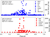 |
Fig. 1. Folded burst-rate distribution for FRB 20121102A at L band (top) and for FRB 20180916B at P band (bottom). The bursts are symbol-coded according to the observing radio telescope. The burst rate was scaled to a reference 100 m telescope using Eq. 3. A full list of the telescopes contributing to the L-band and P-band data can be found in Sect. 2. |
3.1. Von Mises model
Although the active window might indicate a Gaussian-like behaviour, this distribution is not suited for periodic data and would not allow for predictions of future activity cycles. To address this limitation, we adopted a Von Mises distribution, which represents a continuous probability distribution and works to sample circular objects, such as periodic data (Kitagawa & Rowley 2022). The Von Mises distribution is defined as (Mardia & Jupp 2009)
 (6)
(6)
where μ is the position at which the distribution is clustered, κ is a concentration parameter that determines the width and steepness of the curve, and I0(κ) is the modified Bessel function of order zero. This distribution has a dominion of x ∈ [0, 2π], and thus, a conversion was made to map the phase from 0 to 1.
3.2. Chromatic model
Building on the work of Bethapudi et al. (2023), we defined the chromatic activity model using a power-law relation that linked the observing frequency and phase of detected bursts to construct the activity window. The model is described by the following power-law (f(ν)) equation:
 (7)
(7)
where ν is the observed frequency, and ν0 is the reference frequency at which the periodicity model was originally defined. For FRB 20121102A, ν0 = 1360 MHz, and for FRB 20180916B, ν0 = 600 MHz, which both correspond to the centre of the frequency band at which most of the detections are made for each source. The parameters A and B were fitted from the data and indicate the steepness and amplitude of the frequency dependence, respectively.
Importantly, each detection was considered to extend over the full bandwidth of the receiver used in the observation. To account for differences in frequency range and bandwidth among the telescopes in our sample within a given observing band (P, L, S, or C band), we replicated each event every 50 MHz until the full bandwidth of the corresponding instrument was covered. For example, when Effelsberg detected an event using its seven-beam receiver with a 300 MHz bandwidth centred at 1.4 GHz, six data points were added to the sample, each with central frequencies given by
 (8)
(8)
where N is the number of replicated frequency points, calculated as N = ⌊BW/Δν⌋. We adopted a replication step of Δν = 50 MHz, motivated by the typical bandwidth differences among the telescopes in the sample. This procedure provided a smoother frequency coverage than a simple split into the four bands (P, L, S, and C band). We acknowledge that using the observed frequency extent of each burst would be a better approach. Nevertheless, most works do not report this information, and performing an individual analysis for individual burst is beyond the scope of this work.
The chromatic activity window was modelled by splitting the sample into frequency bins and fitting the cumulative distribution function (CDF) of a Von Mises to the phase distribution. The Von Mises distribution returns μ, the peak of the distribution, and κ, the shape parameter that accounts for the steepness in the rise of the distribution. Examples of the fitting process are given in Figs. 2 and 3, where we display the dataset at the reference frequency, 1.36 GHz and 600 MHz, at which most events are detected for FRBs 20121102A and 20180916B, respectively.
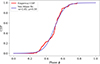 |
Fig. 2. Von Mises CDF fit (purple) to the empirical CDF (red) of FRB 20121102A at 1360 MHz. The fit is centred at a phase μ = 0.5 and shaped by κ = 2.8 |
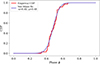 |
Fig. 3. Von Misses CDF fit (purple) to the empirical CDF (red) of FRB 20180916B at 600 MHz. The fit is centred at a phase μ = 0.48 and shaped by κ = 6.4. |
Then, the peak of the fit in each frequency bin, μ, was fitted by a power law across frequency. This curve represents the peak activity of the window across frequencies. The spread around this peak was determined by the phase full width at half maximum (FWHM) of the Von Mises fit, which is related to the duration of the window. The activity window for a given frequency is therefore defined by
![Mathematical equation: $$ \begin{aligned} \phi _{\mathrm{window}}(\nu ) \in \left[ \mu (\nu ) - \frac{{\delta (\nu )}}{2},\ \mu (\nu ) + \frac{{\delta (\nu )}}{2} \right], \end{aligned} $$](/articles/aa/full_html/2026/03/aa56269-25/aa56269-25-eq9.gif) (9)
(9)
with ϕwindow(ν) the phase interval during which an FRB is expected to be active at a given observing frequency ν, μ(ν) the power law fitted through the peaks of the active windows across frequencies (i.e. μ of the Von Mises curve), and δ(ν) was obtained by fitting the power law to the FWHM measured in each frequency bin.
Figure 4 presents an example of the modelled active window of FRB 20121102A at 1360 MHz, based on the chromatic model. The predicted Von Mises distribution is characterised by μ = 0.47 and κ = 4.28. At a 99.7% confidence level, and the width of the active window spans approximately 55% of the cycle (∼87 days). Similarly, for FRB 20180916B, Fig. 5 shows the modelled active window at 600 MHz, with a predicted Von Mises distribution with parameters μ = 0.47 and κ = 9.8. The width of the window is estimated to be approximately 32% of the cycle (∼5 days) at the 99.7% confidence level.
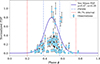 |
Fig. 4. Modelled active window of FRB 20121102A at 1360 MHz. The curve is centred at a phase μ = 0.47 and shaped by κ = 4.28. The dashed-dotted blue limits indicate the FWHM, and the dashed red limits mark the activity window at 99.7% confidence level. Observations are shown with blue points with their respective 3σ uncertainties. |
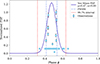 |
Fig. 5. Modelled active window of FRB 20180916B at 600 MHz. The curve is centred at a phase μ = 0.47 and shaped by κ = 9.8. The dashed-dotted blue limits indicate the FWHM, and the dashed red limits mark the activity window at 99.7% confidence level. Observations are shown with blue dots with their respective 3σ uncertainties. |
4. Results
Figs. 6a and 6b presents the chromatic activity windows of FRB 20121102A and FRB 20180916B. For FRB 20121102A, the denser detection region is in the L band, and for FRB 20180916B, the denser region is in the P band.
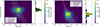 |
Fig. 6. The activity window was constructed using a power-law model that fitted the peaks of the Von Mises distributions across frequency bands. The colour map shows the distribution of detected bursts using a Gaussian kernel density fitted to the data, included for visualisation purposes and normalised to resemble a probability density function. The red curve corresponds to the peak of the activity window and the white limits show its FWHM. The marginal bins, colour-coded by density, display the distribution of burst detections across frequency. For FRB 20121102A (panel a), the fitted parameters are Aμ = −0.195 and Bμ = 0.470, and for FRB 20180916B (panel b), the parameters are Aμ = −0.186 and Bμ = 0.475. |
The frequency band for FRB 20121102A is split into bins 50 MHz wide, ranging from 1 GHz to 8 GHz. For FRB 20180916B, we used frequency bins of 50 MHz in the range of 0.1 GHz to 5 GHz
The results of the power-law fitting for the parameters A and B, as defined in Sect. 3, are summarised in Table 2. These parameters characterise the frequency dependence of the peak phase (μ) and the FWHM (δ) of the activity window, following the power-law relation presented in Sect. 3. Specifically, Aμ and Bμ refer to the fit of the peak phase, and Aδ and Bδ correspond to the FWHM fit.
Best-fit power-law parameters for the activity window of FRBs.
For FRB 20121102A, Fig. 7a shows the predicted activity windows in UTC spanning from January 20, 2026, to April 15, 2027, computed at 1360 MHz. We expect the next active window to begin around February 25, 2026, and to end around May 24. Likewise, Fig. 7b presents the predicted activity windows for FRB 20180916B at 600 MHz, spanning February 2, 2026, to April 28, 2026. The upcoming active cycle is expected to start on February 14, 2026, and to conclude on February 19, 2026.
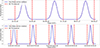 |
Fig. 7. Activity windows modelled using a Von Mises distribution. The dash-dotted red lines indicate the 99.7% confidence level of the activity window. Panel (a): Predicted active windows of FRB 20121102A at 1360 MHz, spanning from January 20, 2026, to April 15, 2027. Panel (b): Predicted active windows of FRB 20180916B at 600 MHz, spanning from February 2, 2026, to April 28, 2026. |
5. Discussion
5.1. Active window behaviour
For FRB 20180916B, the activity window starts earlier at a higher frequency. This is shown by the best-fit parameters for the peak of the active window, which are Aμ = −0.186 ± 0.018 and Bμ = 0.475 ± 0.006, and indicate a clear chromatic dependence. This behaviour was previously reported by Pastor-Marazuela et al. (2021) and Bethapudi et al. (2023), and our results are consistent with theirs while incorporating a larger dataset than was used in these previous studies. Regarding the duration of the activity window, which is defined by the FWHM (δ), there is strong evidence of a narrowing with increasing frequency, indicated by the best-fit parameters (Aδ = −0.444 ± 0.047 and Bδ = 0.120 ± 0.005).
The comparison to the results of Bethapudi et al. (2023) for the peak activity (μ) shows that our power-law fit yields Aμ = −0.186 ± 0.018 and Bμ = 0.475 ± 0.006. These results agree with those reported by Bethapudi et al. (2023), who found Aμ = −0.23 ± 0.05 and Bμ = 0.47 ± 0.02. Both results reveal a statistically significant chromatic trend in the activity peak, with a negative value of Aμ that indicates that the start of the activity begins earlier at higher frequencies. Although our inferred chromaticity is less prominent for FRB 20180916B, it remains statistically consistent with the value reported by Bethapudi et al. (2023) within ∼ 1σ.
In the case of the FWHM, we converted our fitted Bδ parameter to hours using the known FRB 20180916B period. We obtained Aδ = −0.444 ± 0.047 and Bδ = 46 ± 1 h. Bethapudi et al. (2023) reported values of Aδ = −0.35 ± 0.32 and Bδ = 53.4 ± 15.6 h. In our results, the width of the activity window depends significantly on frequency, with a negative slope suggesting a narrower window at higher frequencies. Bethapudi et al. (2023) reported a lesser negative slope, meaning that in comparison with our modelling, their activity is wider at each frequency band, but with a high uncertainty that is statistically consistent with zero. We report lower uncertainties because our sample is larger and because we used the CDF approach, which strengthens the observed behaviour trend. In terms of the amplitude parameter Bδ, our results agree within 1σ.
Regarding FRB 20121102A, our result also suggests a chromatic active window, with the activity starting earlier at a higher frequency (Aμ = −0.195 ± 0.073 and Bμ = 0.470 ± 0.024). In contrast to FRB 20180916B, the FWHM δ of FRB 20121102A widens with increasing frequency (Aδ = 0.112 ± 0.098 and Bδ = 0.185 ± 0.0014).
5.2. FRB comparison
The results of the power-law fitting presented in Table 2 allowed us to compare the chromatic behaviour of FRB 20121102A and FRB 20180916B in terms of the peak phase and the FWHM of the active window, as shown in Fig. 8.
 |
Fig. 8. Comparison of the chromatic activity windows for FRB 20121102A (red) and FRB 20180916B (blue). The solid lines represent the power-law fits to the peak phases of each FRB activity window. For FRB 20121102A, the fit is characterised by Aμ = −0.195 ± 0.073 and Bμ = 0.470 ± 0.024 (red line), and for FRB 20180916B, the fit is given by Aμ = −0.186 ± 0.018 and Bμ = 0.475 ± 0.006 (blue line). The shaded regions represent the FWHM of the active windows. |
The peak activity is similar for the two sources. It has a negative exponent Aμ, which indicates a shift in the activity window towards earlier phases at higher frequencies. FRB 20121102A displays a slightly steeper frequency dependence in its peak phase, with Aμ = −0.195 ± 0.073, compared to FRB 20180916B, for which Aμ = −0.186 ± 0.018, but they agree within their uncertainties. The Bμ values are nearly identical for the two sources (Bμ ∼ 0.47), suggesting a similar scaling of the peaks with frequency.
In contrast, the chromatic behaviour of the FWHM differs between the two sources. For FRB 20121102A, the FWHM exhibits a broadening with increasing frequency, with a positive exponent Aδ. FRB 20180916B shows a narrowing trend, with a negative exponent. The difference in the Bδ exponents indicates that the frequency scaling of the width is stronger for FRB 20121102A than for FRB 20180916B.
These results suggest that while the two sources show a similar frequency dependence in their peak phases overall, that is, they start earlier at higher frequencies, their on-phase behaviours diverge: The active phase of FRB 20121102A broadens at higher frequencies, whereas FRB 20180916B becomes narrower.
5.3. Model discussion
The chromatic model, although simple in nature, allowed us to compare the differences in the activity for FRB 20180916B and FRB 20121102A. Possible model improvements might consider the rate scaling (Sect. 2) using the γ-values reported by each telescope and using the width of the burst dynamic spectra instead of the observing bandwidth as a proxy.
It is important to note that the Von Mises CDF fit does not include information about the expected burst rates, but only about the phase distribution, which limits the amplitude of the curve, as shown in Figs. 4 and 5. Any analysis related to the detection probability should take this limitation into account.
Bands with a small number of detections, such as C (4–8 GHz), are particularly biased in the use of the observing bandwidth as an approximation for the frequency extent of the bursts, which complicates the fitting process because the observing setups at this frequency provide a few GHz wide band in comparison with fractions of GHz at lower frequencies. The C-band detections for the two FRBs are overlaid on the detection contour plot in Fig. 9. In the case of FRB 20121102A, the C band shows that the detections cover most of the active window (∼0.8 of the cycle) and that it starts earlier. This strengthens the findings up to S band of the FRB 20121102A chromaticity. Still, it is important to highlight that the full phase is not mapped. In the case of FRB 20180916B, the detections in C band are extremely clustered in phase, which also impedes a proper fit. The limitations imposed by C band are not new. Braga et al. (2025) also reported the limiting lack of observations for periodicity searches of FRB 20121102A over this frequency band. Further observations across a broader range of frequencies are necessary to fully address these limitations and provide a better understanding of the correlation between phase and frequency of the active window.
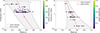 |
Fig. 9. Detections of FRB 20121102A (panel a) and FRB 20180916B (panel b) as scatter points. The colour scale depicts the normalised detection rate, with yellow indicating higher rates or densities. The active window is shown within the 99.7% confidence level. |
We used the Kolmogorov–Smirnov (KS) goodness-of-fit test to evaluate whether the observed burst phase distributions were consistent with a Von Mises model. The KS statistic is defined as the maximum difference between the empirical cumulative distribution function (CDF) of the data and the CDF of the proposed model. In this context, the null hypothesis H0 states that the burst phases are drawn from a Von Mises distribution, while the alternative hypothesis H1 states that the observed phase distribution deviates from this model. In particular, p < 2.7 × 10⁻³ (3σ threshold) rejects the null hypothesis.
We applied the test to each Von Mises CDF fit at each frequency bin and present the results in Fig. 10. For FRB 20180916B, the p values across all frequency bins show no evidence of deviations from the model. For FRB 20121102A, the p values indicate consistency with the model in most frequency bins, with 128 out of 131 frequencies having p values above the commonly used reference levels. In the range of lower frequencies, ∼ 800 MHz to 900 MHz, however, it is not able to characterise the data because the sampling size is too small. We also note that at the highest frequencies, above 4 GHz for FRB 20180916B and above 5 GHz for FRB 20121102A, the p values may be biased, again because of the small sample sizes in these bins.
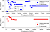 |
Fig. 10. p values of KS goodness-of-fit tests comparing Von Mises cumulative distribution function (CDF) models to the empirical phase CDFs, shown for each frequency bin of FRB 20121102A (top) and FRB 20180916B (bottom). For each frequency bin, the p value quantifies whether the observed burst phase distribution is consistent with a Von Mises model. The dashed horizontal line marks the 3σ rejection threshold (p = 2.7 × 10⁻³); values below this line indicate that the Von Mises model is statistically rejected. The inset highlights the p values in the lowest-frequency bins for FRB 20121102A. |
Although scaled rates depend on the γ index value, we observed no significant change in the power-law fitting results when we tested the range of γ = −1.1 to −1.8 for FRB 20121102 or the γ range of −0.5 to −1.4 for FRB 20180916B.
5.4. Model implications
The finding of chromaticity in FRB 20180916B imposed a constraint on progenitors models; models had to explain activity that started earlier and narrowed at higher frequencies. Li & Zanazzi (2021) proposed that the chromatic behaviour of FRB 20180916B is consistent with theories where the periodicity is given by a slowly rotating or freely precessing magnetar. This mechanism is based on radius-to-frequency mapping (RFM) or altitude-dependent emission. The emissions at lower frequency originate at a higher altitude in the magnetosphere, where the lines of magnetic field diverge, creating an wider emission cone. The chromatic behaviour would arise from the emission cone staying aligned with the observer for longer, and the phase drift would be due to the higher magnetic polar angles observed at lower frequency bands.
Wadiasingh & Timokhin (2019) proposed ultra-long period magnetars (ULPMs) as an explanation for repeating FRBs, where stress accumulates in a low-twist magnetosphere and is released during short magnetar bursts, producing coherent radio emission that escapes as FRBs. Building on this framework, Bilous et al. (2025) applied the ULPM model to FRB 20201124A, which resembles the chromatic behaviour of FRB 20180916B. In the model, the RFM is used to explain the frequency dependence of the active window, but the authors noted a large difference in timescales for which the model must account. While pulsar active windows last fractions of a second, FRB activity windows can last for days. The authors argued that this discrepancy can be naturally resolved if FRBs originate from ULPMs with spin periods of several weeks or longer.
In addition to the long periodicity, FRB 20121102A introduces a new challenge; the broadening of the activity window at higher frequencies. Lyutikov et al. (2020) proposed a binary comb model (BCM) that is generated when a pulsar orbits a massive O/B star and interacts with its wind. The periodicity arises from the free-free absorption in the primary wind of the star. The stellar wind is optically thick and too dense for radio waves, and a transparency funnel in the stellar wind is thus created by the pulsar. The bursts would only be visible when the line of sight is aligned with this cone. Since the free-free strongly depends on frequency, the wind will become more transparent at higher frequencies, which would allow bursts to escape from a wider range of angles. This would create an extended active window at a higher frequency.
Ioka & Zhang (2020) included two additional opacity models for the BCM. The fist model is the τ-crossing mode, where the orbit intersects the photosphere, the pulsar FRB enters and exits the photosphere periodically, and the periodicity is explained by the temporal variation of the optical depth. The second model is the inverse funnel mode, in which the companion wind plunges into the wind of the pulsar FRB, inverting the direction of the funnel. In both of these cases, the implication is that the active window is wider at higher frequencies.
While FRB 20180916B shows a narrowing activity window at higher frequencies, seemingly contradicting the BCM predictions, FRB 20121102A presents a chromatic behaviour that is consistent with the model. Progenitor models must reconcile these differences within a single framework. Importantly, it should be differentiated whether the window dependence with frequency is intrinsic to the emission, due to propagation, or due to an observational bias Wada et al. (2021).
5.5. Isotropic energy
With the dataset, we also corroborated whether the burst properties exhibit a phase-dependent behaviour. We analysed the distribution of isotropic burst energies, the waiting times, and the burst width for FRB 20121102A as a function of activity phase.
We considered a subset of the data described in Sect. 2, specifically, from Jahns et al. (2023) and Li et al. (2021), where sub-bursts were excluded for simplicity. The energy values in these two samples were originally computed using different methods: Li et al. (2021) used the central observing frequency, whereas Jahns et al. (2023) scaled the burst fluences to account for signal components extending beyond the observing bandwidth. To ensure consistency across the dataset, we re-calculated the isotropic energy for all bursts using the expression
 (10)
(10)
where DL is the luminosity distance, F is the fluence in Jy s, BW the bandwidth in Hz, and z is the redshift. The ToA between bursts were calculated as the difference in arrival time of two bursts wti = ToAi + 1 − ToAi. The fluences were obtained from the datasets provided by the studies. In the case of Li et al. (2021), the fluences were measured using the peak flux density and equivalent burst duration, and for Jahns et al. (2023), they were calculated using an SEFD dependent on frequency and zenith angle.
We performed simple correlation tests for each parameter (E, ToA, and burst width) and the activity phase. In general, the correlation between parameters and phase is negligible, except for the isotropic energy shown in Fig. 11. We tested the combined dataset and the Li et al. (2021) and Jahns et al. (2023) samples independently, first using a circular distance metric between the burst phase and the centre of the activity window. This was motivated by the results for FRB 20180916B, whose bursts energy seems to peak in middle of the activity window (Bhattacharyya et al. 2024). In the Li et al. (2021) sample, we found a positive correlation between the isotropic energy and the distance to the window centre (Spearman ρ = 0.278, p = 1.2 × 10⁻³⁰; Kendall τ = 0.178, p = 2.7 × 10⁻²⁷), indicating that higher-energy bursts preferentially occur away from the centre. A weaker but still significant trend was observed for the combined dataset (Spearman ρ = 0.141, p = 5.4 × 10⁻¹²), while no significant correlation was found in the Jahns et al. (2023) sample. The difference probably arises because the Li et al. (2021) sample spans most of the activity window, but includes fewer bursts near the end, whereas the Jahns et al. (2023) sample predominantly covers the later half of the window and exhibits a more dispersed phase distribution.
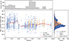 |
Fig. 11. Phase–resolved burst energetics of FRB 20121102A. The central panel shows the isotropic burst energy as a function of activity phase for the Li et al. (2021) and Jahns et al. (2023) samples. The solid red curve traces the phase-binned median energy, with the shaded region indicating the 1σ bootstrap uncertainty based on 10 000 resamples. The top panel shows the total number of bursts per phase bin. The burst phases were computed assuming a 159.3-day activity period, with a reference epoch MJDref = 58356.5 corresponding to ϕref = 0 (Braga et al. 2025). The right panel displays the marginal energy distributions for the two samples; the Li et al. (2021) sample is described by a bimodal Gaussian with peaks at E ≃ 1.8 × 1037 (dashed blue curve) and 1.2 × 1038 erg (dotted blue curve), while the Jahns et al. (2023) sample is consistent with a single Gaussian peaking at E ≃ 4.0 × 1037 erg (red curve). |
The circular distance test does not distinguish between the beginning and end of the activity window, however, and we therefore further tested for a monotonic dependence of the energy on phase. We found a negative trend in the Li et al. (2021) sample (Spearman ρ = −0.271, p = 3.5 × 10⁻²⁹), which implies that the burst energies are higher at earlier phases and decrease toward the end of the activity window. This trend is also supported by the phase-binned median energy shown in Fig. 11 with the red line (1σ bootstrap uncertainties), which peaks away from the centre of the activity window. Importantly, the phase-resolved burst rate (top panel) shows that the centre of the activity window contains the highest number of detected bursts, but corresponds to one of the lowest median energies. This demonstrates that the observed trend is not necessarily due to variations in burst rate.
These results indicate a mild preference for more energetic bursts occurring at the beginning of the activity window in FRB 20121102A overall, in contrast to FRB 20180916B, where the burst energy has been reported to peak near the centre of the activity cycle (Bhattacharyya et al. 2024).
6. Conclusions
We presented the modelling of the chromatic activity windows of two periodically repeating FRBs, FRB 20121102A and FRB 20180916B. The chromaticity was modelled using a combination of a Von Mises distribution to model the phase and a power-law relation to model the frequency dependence, as described in Sect. 3. To construct the models, we used publicly available data of the sources as listed in Sect. 2, and we divided these data by frequency bands. The detections in Figs. 6a and 6b cover a range of .1–8 GHz.
The two FRBs display a shift in peak activity to earlier phases at higher frequencies, although their steepness differs, with FRB 20121102A displaying a slightly steeper dependence on frequency than FRB 20180916B, as shown in Fig. 8. For FRB 20121102A, however, the widening in the activity window occurs at higher frequencies than for FRB 20180916B, which displays a broadening at lower frequencies. For FRB 20180916B, the chromatic behaviour agrees with the behaviour presented by Bethapudi et al. (2023). For FRB 20121102A, this is a newly reported feature.
The difference between these two periodic FRBs is also reflected in the isotropic energy distributions of their bursts. For FRB 20180916B, the median burst energy has been reported to peak near the centre of the activity window, where we found evidence for more energetic bursts from FRB 20121102A at the beginning of the activity window. An in-depth modelling of the observational biases and a more homogeneous sampling of the active window is required to robustly confirm these trends.
Acknowledgments
This research started during a summer internship conducted at the Max-Planck-Institut für Radioastronomie, M.C.E extends her gratitude to M. Kramer and his research group, in particular to L. Spitler and S. Bethapudi for useful discussions. The authors thank the anonymous referee for their valuable comments on the manuscript that helped improve its quality. M.C.E thanks I. Crosby for the feedback. M. C acknowledges support from Max Planck Society through the Max Planck Parter Group at UC and CIA250016 (CPS-RTC). T.C. gratefully acknowledges support by the ANID BASAL FB210003.
References
- Bethapudi, S., Spitler, L., Main, R., Li, D., & Wharton, R. 2023, MNRAS, 524, 3303 [NASA ADS] [CrossRef] [Google Scholar]
- Bethapudi, S., Spitler, L. G., Li, D. Z., et al. 2025, A&A, 694, A75 [NASA ADS] [CrossRef] [EDP Sciences] [Google Scholar]
- Bhattacharyya, S., Roy, J., & Bera, A. 2024, ArXiv e-print [arXiv:2409.20307] [Google Scholar]
- Bilous, A. V., van Leeuwen, J., Maan, Y., et al. 2025, A&A, 696, A194 [NASA ADS] [CrossRef] [EDP Sciences] [Google Scholar]
- Braga, C. A., Cruces, M., Cassanelli, T., et al. 2025, A&A, 693, A40 [NASA ADS] [CrossRef] [EDP Sciences] [Google Scholar]
- Caleb, M., Stappers, B. W., Abbott, T. D., et al. 2020, MNRAS, 496, 4565 [NASA ADS] [CrossRef] [Google Scholar]
- Cassanelli, T., Leung, C., Sanghavi, P., et al. 2024, Nat. Astron., 8, 1429 [Google Scholar]
- Chatterjee, S., Law, C., Wharton, R., et al. 2017, Nature, 541, 58 [NASA ADS] [CrossRef] [Google Scholar]
- CHIME/FRB Collaboration (Amiri, M., et al.) 2020a, Nature, 582, 351 [NASA ADS] [CrossRef] [Google Scholar]
- CHIME/FRB Collaboration (Andersen, B. C., et al.) 2020b, Nature, 587, 54 [Google Scholar]
- Cruces, M., Spitler, L., Scholz, P., et al. 2021, MNRAS, 500, 448 [Google Scholar]
- Cruces, M., Spitler, L. G., Scholz, P., et al. 2021, MNRAS, 500, 448 [Google Scholar]
- Feng, Y., Jiang, J., Zhou, D., et al. 2023, ATel., 15980, 1 [Google Scholar]
- Gajjar, V., Siemion, A. P. V., Price, D. C., et al. 2018, ApJ, 863, 2 [NASA ADS] [CrossRef] [Google Scholar]
- Gourdji, K., Michilli, D., Spitler, L., et al. 2019, ApJ, 877, L19 [NASA ADS] [CrossRef] [Google Scholar]
- Hardy, L. K., Dhillon, V. S., Spitler, L. G., et al. 2017, MNRAS, 472, 2800 [NASA ADS] [CrossRef] [Google Scholar]
- Hewitt, D. M., Snelders, M. P., Hessels, J. W. T., et al. 2022, MNRAS, 515, 3577 [NASA ADS] [CrossRef] [Google Scholar]
- Hilmarsson, G., Michilli, D., Spitler, L., et al. 2021, ApJ, 908, L10 [NASA ADS] [CrossRef] [Google Scholar]
- Houben, L. J. M., Spitler, L. G., ter Veen, S., et al. 2019, A&A, 623, A42 [NASA ADS] [CrossRef] [EDP Sciences] [Google Scholar]
- Ioka, K., & Zhang, B. 2020, ApJ, 893, L26 [NASA ADS] [CrossRef] [Google Scholar]
- Jahns, J. N., Spitler, L. G., Nimmo, K., et al. 2023, MNRAS, 519, 666 [Google Scholar]
- Josephy, A., Chawla, P., Fonseca, E., et al. 2019, ApJ, 882, L18 [NASA ADS] [CrossRef] [Google Scholar]
- Kitagawa, T., & Rowley, J. 2022, ArXiv preprint [arXiv:2202.05192] [Google Scholar]
- Law, C. J., Abruzzo, M. W., Bassa, C. G., et al. 2017, ApJ, 850, 76 [Google Scholar]
- Law, C. J., Connor, L., & Aggarwal, K. 2022, ApJ, 927, 55 [NASA ADS] [CrossRef] [Google Scholar]
- Li, D., & Zanazzi, J. J. 2021, ApJ, 909, L25 [Google Scholar]
- Li, D., Wang, P., Zhu, W. W., et al. 2021, Nature, 598, 267 [CrossRef] [Google Scholar]
- Locatelli, N., Ronchi, M., Ghirlanda, G., & Ghisellini, G. 2019, A&A, 625, A109 [NASA ADS] [CrossRef] [EDP Sciences] [Google Scholar]
- Lorimer, D. R., & Kramer, M. 2004, Handbook of Pulsar Astronomy, 4 [Google Scholar]
- Lorimer, D. R., Bailes, M., McLaughlin, M. A., Narkevic, D. J., & Crawford, F. 2007, Science, 318, 777 [Google Scholar]
- Lyutikov, M., Barkov, M. V., & Giannios, D. 2020, ApJ, 893, L39 [NASA ADS] [CrossRef] [Google Scholar]
- Majid, W. A., Pearlman, A. B., Nimmo, K., et al. 2020, ApJ, 897, L4 [NASA ADS] [CrossRef] [Google Scholar]
- Marcote, B., Paragi, Z., Hessels, J. W. T., et al. 2017, ApJ, 834, L8 [CrossRef] [Google Scholar]
- Marcote, B., Kirsten, F., Hessels, J., Nimmo, K., & Paragi, Z. 2022, PoS, EVN2021, 035 [Google Scholar]
- Mardia, K., & Jupp, P. 2009, Directional Statistics, Wiley Series in Probability and Statistics (Wiley) [Google Scholar]
- Michilli, D., Seymour, A., Hessels, J. W. T., et al. 2018, Nature, 553, 182 [Google Scholar]
- Oostrum, L. C., Maan, Y., van Leeuwen, J., et al. 2020, A&A, 635, A61 [NASA ADS] [CrossRef] [EDP Sciences] [Google Scholar]
- Pal, A. 2025, ApJ, 983, L15 [Google Scholar]
- Pastor-Marazuela, I., Connor, L., van Leeuwen, J., et al. 2021, Nature, 596, 505 [NASA ADS] [CrossRef] [Google Scholar]
- Pearlman, A. B., Majid, W. A., Prince, T. A., et al. 2020, ApJ, 905, L27 [NASA ADS] [CrossRef] [Google Scholar]
- Petroff, E., Hessels, J., & Lorimer, D. 2022, A&ARv., 30, 2 [NASA ADS] [CrossRef] [Google Scholar]
- Pleunis, Z., Michilli, D., Bassa, C. G., et al. 2021, ApJ, 911, L3 [NASA ADS] [CrossRef] [Google Scholar]
- Rajwade, K. M., Mickaliger, M. B., Stappers, B. W., et al. 2020, MNRAS, 495, 3551 [NASA ADS] [CrossRef] [Google Scholar]
- Sand, K. R., Faber, J. T., Gajjar, V., et al. 2022, ApJ, 932, 98 [NASA ADS] [CrossRef] [Google Scholar]
- Scholz, P., Spitler, L. G., Hessels, J. W. T., et al. 2016, ApJ, 833, 177 [CrossRef] [Google Scholar]
- Scholz, P., Bogdanov, S., Hessels, J. W. T., et al. 2017, ApJ, 846, 80 [NASA ADS] [CrossRef] [Google Scholar]
- Spitler, L. G., Cordes, J. M., Hessels, J. W. T., et al. 2014, ApJ, 790, 101 [NASA ADS] [CrossRef] [Google Scholar]
- Spitler, L., Scholz, P., Hessels, J., et al. 2016, Nature, 531, 202 [NASA ADS] [CrossRef] [Google Scholar]
- Spitler, L. G., Scholz, P., Hessels, J. W. T., et al. 2016, Nature, 531, 202 [NASA ADS] [CrossRef] [Google Scholar]
- Spitler, L. G., Herrmann, W., Bower, G. C., et al. 2018, ApJ, 863, 150 [NASA ADS] [CrossRef] [Google Scholar]
- Tendulkar, S. P., Bassa, C., Cordes, J. M., et al. 2017, ApJ, 834, L7 [NASA ADS] [CrossRef] [Google Scholar]
- Wada, T., Ioka, K., & Zhang, B. 2021, ApJ, 920, 54 [NASA ADS] [CrossRef] [Google Scholar]
- Wadiasingh, Z., & Timokhin, A. 2019, ApJ, 879, 4 [NASA ADS] [CrossRef] [Google Scholar]
- Xu, J., Feng, Y., Li, D., et al. 2023, Universe, 9, 330 [NASA ADS] [CrossRef] [Google Scholar]
- Zhang, B. 2018, ApJ, 867, L21 [NASA ADS] [CrossRef] [Google Scholar]
- Zhang, B. 2023, Rev. Modern Phys., 95, 035005 [Google Scholar]
- Zhang, Y.-K., Li, D., Feng, Y., et al. 2024, Sci. Bull., 69, 1020 [NASA ADS] [CrossRef] [Google Scholar]
All Tables
All Figures
|
Fig. 1. Folded burst-rate distribution for FRB 20121102A at L band (top) and for FRB 20180916B at P band (bottom). The bursts are symbol-coded according to the observing radio telescope. The burst rate was scaled to a reference 100 m telescope using Eq. 3. A full list of the telescopes contributing to the L-band and P-band data can be found in Sect. 2. |
| In the text | |
|
Fig. 2. Von Mises CDF fit (purple) to the empirical CDF (red) of FRB 20121102A at 1360 MHz. The fit is centred at a phase μ = 0.5 and shaped by κ = 2.8 |
| In the text | |
|
Fig. 3. Von Misses CDF fit (purple) to the empirical CDF (red) of FRB 20180916B at 600 MHz. The fit is centred at a phase μ = 0.48 and shaped by κ = 6.4. |
| In the text | |
|
Fig. 4. Modelled active window of FRB 20121102A at 1360 MHz. The curve is centred at a phase μ = 0.47 and shaped by κ = 4.28. The dashed-dotted blue limits indicate the FWHM, and the dashed red limits mark the activity window at 99.7% confidence level. Observations are shown with blue points with their respective 3σ uncertainties. |
| In the text | |
|
Fig. 5. Modelled active window of FRB 20180916B at 600 MHz. The curve is centred at a phase μ = 0.47 and shaped by κ = 9.8. The dashed-dotted blue limits indicate the FWHM, and the dashed red limits mark the activity window at 99.7% confidence level. Observations are shown with blue dots with their respective 3σ uncertainties. |
| In the text | |
|
Fig. 6. The activity window was constructed using a power-law model that fitted the peaks of the Von Mises distributions across frequency bands. The colour map shows the distribution of detected bursts using a Gaussian kernel density fitted to the data, included for visualisation purposes and normalised to resemble a probability density function. The red curve corresponds to the peak of the activity window and the white limits show its FWHM. The marginal bins, colour-coded by density, display the distribution of burst detections across frequency. For FRB 20121102A (panel a), the fitted parameters are Aμ = −0.195 and Bμ = 0.470, and for FRB 20180916B (panel b), the parameters are Aμ = −0.186 and Bμ = 0.475. |
| In the text | |
|
Fig. 7. Activity windows modelled using a Von Mises distribution. The dash-dotted red lines indicate the 99.7% confidence level of the activity window. Panel (a): Predicted active windows of FRB 20121102A at 1360 MHz, spanning from January 20, 2026, to April 15, 2027. Panel (b): Predicted active windows of FRB 20180916B at 600 MHz, spanning from February 2, 2026, to April 28, 2026. |
| In the text | |
|
Fig. 8. Comparison of the chromatic activity windows for FRB 20121102A (red) and FRB 20180916B (blue). The solid lines represent the power-law fits to the peak phases of each FRB activity window. For FRB 20121102A, the fit is characterised by Aμ = −0.195 ± 0.073 and Bμ = 0.470 ± 0.024 (red line), and for FRB 20180916B, the fit is given by Aμ = −0.186 ± 0.018 and Bμ = 0.475 ± 0.006 (blue line). The shaded regions represent the FWHM of the active windows. |
| In the text | |
|
Fig. 9. Detections of FRB 20121102A (panel a) and FRB 20180916B (panel b) as scatter points. The colour scale depicts the normalised detection rate, with yellow indicating higher rates or densities. The active window is shown within the 99.7% confidence level. |
| In the text | |
|
Fig. 10. p values of KS goodness-of-fit tests comparing Von Mises cumulative distribution function (CDF) models to the empirical phase CDFs, shown for each frequency bin of FRB 20121102A (top) and FRB 20180916B (bottom). For each frequency bin, the p value quantifies whether the observed burst phase distribution is consistent with a Von Mises model. The dashed horizontal line marks the 3σ rejection threshold (p = 2.7 × 10⁻³); values below this line indicate that the Von Mises model is statistically rejected. The inset highlights the p values in the lowest-frequency bins for FRB 20121102A. |
| In the text | |
|
Fig. 11. Phase–resolved burst energetics of FRB 20121102A. The central panel shows the isotropic burst energy as a function of activity phase for the Li et al. (2021) and Jahns et al. (2023) samples. The solid red curve traces the phase-binned median energy, with the shaded region indicating the 1σ bootstrap uncertainty based on 10 000 resamples. The top panel shows the total number of bursts per phase bin. The burst phases were computed assuming a 159.3-day activity period, with a reference epoch MJDref = 58356.5 corresponding to ϕref = 0 (Braga et al. 2025). The right panel displays the marginal energy distributions for the two samples; the Li et al. (2021) sample is described by a bimodal Gaussian with peaks at E ≃ 1.8 × 1037 (dashed blue curve) and 1.2 × 1038 erg (dotted blue curve), while the Jahns et al. (2023) sample is consistent with a single Gaussian peaking at E ≃ 4.0 × 1037 erg (red curve). |
| In the text | |
Current usage metrics show cumulative count of Article Views (full-text article views including HTML views, PDF and ePub downloads, according to the available data) and Abstracts Views on Vision4Press platform.
Data correspond to usage on the plateform after 2015. The current usage metrics is available 48-96 hours after online publication and is updated daily on week days.
Initial download of the metrics may take a while.