| Issue |
A&A
Volume 707, March 2026
|
|
|---|---|---|
| Article Number | A39 | |
| Number of page(s) | 8 | |
| Section | The Sun and the Heliosphere | |
| DOI | https://doi.org/10.1051/0004-6361/202556599 | |
| Published online | 25 February 2026 | |
Exploring spatial and temporal patterns across solar cycles: Focusing on active longitudes
1
Department of Astronomy, Eötvös Loránd University Pázmány Péter sétány 1/A H-1117 Budapest, Hungary
2
University of Sheffield, School of Electrical and Electronic Engineering, Amy Johnson Building Portabello Street Sheffield S1 3JD, UK
3
Gyula Bay Zoltán Solar Observatory (GSO), Hungarian Solar Physics Foundation (HSPF) Petőfi tér 3 H-5700 Gyula, Hungary
4
Solar Physics and Space Plasma Research Centre, School of Mathematical and Physical Sciences, University of Sheffield, Hicks Building Hounsfield Road S3 7RH, UK
★ Corresponding author: This email address is being protected from spambots. You need JavaScript enabled to view it.
Received:
25
July
2025
Accepted:
31
October
2025
Abstract
Context. Active longitudes (ALs) are proposed behavioural patterns on the Sun, whereby certain solar phenomena tend to appear at preferred longitudes, with these longitudes shifting over time on a scale of a few Carrington rotations (CRs). The existence of ALs remains a topic of debate, largely due to our limited understanding of their origin, evolution, and physical significance.
Aims. This study aims to provide support and further evidence towards the existence of ALs by utilising longer-term sunspot and solar flare datasets. As part of this effort, an artificial test dataset for control was also constructed in which the longitudes of sunspots were randomised, allowing a direct comparison with the observational data.
Methods. Kernel density estimation (KDE) was employed to search for longitudinal groupings of sunspot groups and flares on synoptic maps. Furthermore, we explored larger-scale structures by applying a 2D KDE to the peaks of the 1D KDEs (longitude as a function of CR). Finally, we generated artificial solar cycles by simulating sunspots with randomised properties, most notably assigning longitudes from a uniform distribution.
Results. Distinguishable features were identified in the 2D KDEs, showing that during certain periods of the solar cycle, a specific longitude range may exhibit heightened activity, which can later switch off entirely, and a new one can appear ∼180° away, consistent with the AL’s flip-flop effect. Although our randomised datasets also exhibited ALs in their 2D KDEs, these differed notably from the observed patterns: inactive longitudes were less pronounced, and active patches appeared shorter-lived and more numerous. We also identified a parameter for a qualitative comparison: the number of KDE peaks (in the 1D KDE) per number of CRs in a solar cycle. This indicator shows a markedly different distribution between the randomised and observed datasets, confirmed by a Cucconi test p value of 0.0177.
Key words: Sun: activity / Sun: evolution / Sun: flares / Sun: general / sunspots
© The Authors 2026
 Open Access article, published by EDP Sciences, under the terms of the Creative Commons Attribution License (https://creativecommons.org/licenses/by/4.0), which permits unrestricted use, distribution, and reproduction in any medium, provided the original work is properly cited.
This article is published in open access under the Subscribe to Open model. This email address is being protected from spambots. You need JavaScript enabled to view it. to support open access publication.
1. Introduction
Sunspots are the primary tracers of variations in the 11-year solar cycle, and as such, their properties have been extensively studied (Hathaway 2015). Due to their relative ease of observation, detailed catalogues exist going as far back as 1874 (Mandal et al. 2020). Sunspots tend to form groups and these often complex features are also good proxies of solar activity. The areas around and including the sunspots are called active regions (ARs), and a range of phenomena (such as solar flares and coronal mass ejections (CMEs)) correlate with their location and size (Tian 2022; Toriumi et al. 2017; Wang & Zhang 2008). Studying the spatial and temporal occurrence of sunspots, their groups, and the ARs can lead us to a deeper understanding of the solar dynamo, and thereby to a deeper understanding of space weather.
Another well-known phenomenon on the Sun is solar flares, which are strongly connected to sunspots and can have significant effects on the near-Earth environment (Buzulukova & Tsurutani 2022). Solar flares emit intense electromagnetic radiation across the entire spectrum, from radio waves to X-rays and gamma rays (Schrijver 2009). These energetic bursts can disrupt, for example, high-frequency radio communications, especially on the sunlit side of Earth. When a large flare is associated with a CME directed towards Earth, it may lead to geomagnetic storms (Mugatwala et al. 2024). These storms can then disrupt power grids, degrade GPS accuracy, and affect pipeline and railway systems (Vourlidas et al. 2019). The strongest ones (and therefore the most dangerous) have been shown to originate from ARs (Benz 2017), providing further reason to study sunspots.
Spatially, sunspot activity not only adheres to the well-known latitudinal migration depicted in the butterfly diagram (Hathaway 2015) but also exhibits a tendency for ARs to cluster at preferential longitudes, referred to as active longitudes (ALs). This concept has been extensively studied since the early 20th century, with significant contributions from researchers such as Losh (1939), Bogart (1982), Berdyugina & Usoskin (2003), and Zhang et al. (2011), among others. Studies on ALs have consistently suggested that various solar activity indicators, including for example, the sunspots, the global magnetic field (Benevolenskaya et al. 1999; Bumba et al. 2000), the heliospheric magnetic field (Ruzmaikin et al. 2001; Mursula & Hiltula 2004), and solar flares (Bai 1988, 2003; Bumba & Howard 1969; Gyenge et al. 2016), show a pronounced preference for specific, continuously changing longitudinal ranges, thereby reinforcing the idea of ALs.
Furthermore, several studies have shown that ARs disobeying the hemispheric helicity rule appear to form activity nests or ALs (Canfield & Pevtsov 1998; Pevtsov & Canfield 1999, 2000; Zhang & Bao 1999; Tian et al. 2001; Pevtsov & Balasubramaniam 2003). Additionally, Korsós et al. (2024) provided observational evidence that ALs could be important in predicting the upcoming solar storm seasons.
Active longitudes are typically observed to be 20–60 degrees wide (Bai 1988, 2003; Bumba & Howard 1969; Gyenge et al. 2016), lasting for about 10–15 Carrington rotations (CRs, Elek et al. 2024). Gaizauskas et al. (1983) noted that the magnetic complexity of the solar activity within these ALs are sustained by the frequent emergence of new magnetic fluxes. Nevertheless, the underlying mechanisms driving these spatio-temporal patterns remain a subject of ongoing debate.
In this study, we aim to provide observational evidence of ALs by utilising long-term sunspot and flare datasets similar, but on a longer dataset as in Korsós & Erdélyi (2025), including sunspot data spanning more than eleven solar cycles and flare data covering eight solar cycles. These catalogues are discussed in Sect. 2. The analysis methods used to extract information from the raw observations as well as our results are described in Sect. 3. Last but not least, we dissect the implications of our findings as well as briefly address some relevant future outlooks in Sect. 4.
2. Data
2.1. Sunspot group data
The data used for sunspot groups in this study come from the database described in Mandal et al. (2020). The authors composed their catalogue utilising daily observations combined from data from a total of nine observatories, which are: RGO (Royal Greenwich Observatory), Kislovodsk, Pulkovo, Debrecen, SOON (Solar Observing Optical Network), Kodaikanal, Rome, Catania, and Yunnan. This new dataset encompasses the full period between 1874 and 2019, i.e. from the second half of Solar Cycle 11 to the beginning of Solar Cycle 25. The bulk of this period is covered by observations from the RGO and its multiple observing stations around the planet.
The dataset includes the exact observation times, the projection-corrected areas of the sunspot groups in millionths of a solar hemisphere (μHem), their apparent locations in heliographic co-ordinates, and the observatory it was recorded at. For this analysis here, we used all the aforementioned information, with the sole exception of the observatory of origin.
It is also important to note that a direct comparison between each group across multiple datasets was not performed with full precision by Mandal et al. (2020), as it would require one to identify the same group across different sources and account for the evolution of each group. However, this limitation is not a major concern for our analysis, as our primary focus is on identifying general trends in longitudinal grouping rather than examining; for example, the areas of individual groups.
2.2. Flare data
To identify the strong flare activity periods of most of a given solar cycle, two types of catalogues were used. These two flare catalogues are the Hα SOON and X-ray GOES (Geostationary Operational Environmental Satellite).
Prior to the advent of space exploration, solar flares were monitored using Hα filters, a practice dating back to 1938. This method relies on the red spectral line at a wavelength of 656.28 nm, emitted by hydrogen atoms, to classify flares based on their size in square degrees, as was detailed in Benz (2008). Flares are categorised as S for small, with additional classifications of 1 through 4 indicating increasing sizes. Specifically, classifications 3 and 4 denote flares with a visible area exceeding 12.5 square degrees. For this research, covering the period from 1938 to 1974, the focus is exclusively on flares classified as 3 and 4 in size, utilising data from the Hα SOON1 catalogue.
The catalogue of the X-ray GOES2 spans from 1975 to today and includes classifications for solar flares based on the maximum X-ray flux measured near Earth, ranging from wavelengths of 0.1 to 0.8 nm. These classifications categorise flares into five intensity levels: A, B, C, M, and X, with M and X being the most intense. Consequently, the analysis in this study focuses solely on M and X flares to examine periods of significant solar flare activity within each solar cycle.
The above two classification schemes could be matched with each other in general, as was suggested in Bhatnagar & Livingston (2005). Furthermore, these two catalogues also provide information on the occurrence time and position of the flares.
3. Analyses and results
Let us construct synoptic maps from the sunspot and flare catalogues, as a first step, described in Sect. 2. We selected a fixed 10° longitudinal window, defined as a belt of ±5° from the central meridian. The selected 10° band reduces the possibility of counting the same AR twice, as the applied catalogues have daily temporal resolution, while an AR travels about ∼13° per day. Each event was assigned a Carrington longitude based on the time elapsed since the start of the corresponding CR. The latitudes of both sunspots and flares were taken directly from their respective catalogues.
This process resulted in synoptic maps for nearly 2000 CRs, covering the period from 1874 to 2019. Using these maps, we searched for the presence of ALs. To achieve this, kernel density estimation was applied to the data of each synoptic map. This is a non-parametric statistical method that estimates the probability density function of a continuous random variable based on observed data (Rosenblatt 1956; Parzen 1962). Unlike histograms, which approximate data distributions discretely through binning, KDE offers a smooth and continuous representation. This is particularly advantageous for visualising and analysing data in N-dimensional spaces, as it highlights regions of varying probability densities by evaluating the spatial distribution of data points.
In kernel density estimation, each data point contributes a kernel function – typically modelled as a Gaussian distribution – centred on the data point itself. The resulting KDE is the superposition of all individual kernels, producing a smooth estimate of the underlying probability density. A critical aspect of this method may be the choice of the bandwidth parameter, which is a dimensionless scaling factor determining the width (meaning the σ parameter of the Gaussian) of each individual kernel and, consequently, controls the smoothness of the final density curve. A smaller, narrower bandwidth results in a highly detailed estimate that closely follows the data points, potentially obscuring broader trends. Conversely, a larger, broader bandwidth produces a smoother, more generalised curve, but risks over smoothing and producing an almost featureless distribution, thereby concealing important features. The bandwidths are relative to the range of the dataset, meaning that if the dataset spans a wide interval (e.g. from 0 to 100), the same bandwidth will result in less smoothing than if the dataset spans a narrower range (e.g. from 0 to 10). This is why the choice of bandwidth should be adapted to the scale of the data. In the context of this analysis, the selection of an appropriate bandwidth is crucial.
In the scipy.stats.gaussian_kde function, there are built-in methods for determining this bandwidth automatically; namely, the Scott and Silverman methods. However, for the purposes of this work, they both have given dis-satisfactory results, meaning the bandwidths were too broad in both cases. Given the goal of identifying potential ALs with characteristic widths of approximately 20°, the bandwidth must strike a balance: it should be broad enough to group nearby sunspot groups, yet fine enough to resolve distinct ALs. After several trials and errors, the bandwidth parameter was ultimately selected by visual inspection to best satisfy these criteria. We deemed this appropriate, as a difference of bandwidth by even over 10% in either direction would not change our conclusions.
We applied KDE to the entire longitude time series of the sunspot data. We used Python’s scipy module and the stats.gaussian_kde3 function within it. We created the longitude data series using values of [0° ;360° ] for the first CR, then added n ⋅ 360° for each subsequent CR, where n denotes the serial number of the CR after the first one (CR 275). We took the KDE of this 1D data series, using the sizes of the sunspot groups as weights, and applied a bandwidth of 0.00016, which was found to be the most suitable. We have aimed for a common KDE across all data points, resulting in a unified normalisation that enables direct comparisons between different solar cycles, as well as between CRs. This would not be the case if KDEs were calculated separately cycle by cycle, or even less so CR by CR.
After the KDE computation, we subtracted n ⋅ 360° from the resulting array’s x axis. The results were plotted by year onto ridge plots (see Fig. 1), with one panel for each CR within that year. In Fig. 1, the smooth curves are derived from the 1D KDE applied to sunspot-group longitudes. Black dots mark the peaks of the KDEs, indicating the longitudes with the highest probability of sunspot occurrence. The y axes of the individual stripes display the KDE probability density; exact values are omitted for clarity. These axes use arcsinh scaling to represent both small and large differences comparably.
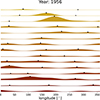 |
Fig. 1. Ridge plot showing the longitudinal distribution of sunspot group activity during the year 1956. Each strip represents a single CR within the year. Note that they do not necessarily begin or end in that year. The x axis shows Carrington longitude within the individual CRs shown, while the y axis is proportional to the probability density determined by the KDE. |
The KDE analysis was also applied to the to the entire longitude time series of the flare data, using the flare class as a weighting factor. A scaling factor of 10 was applied between consecutive classes (e.g. between M1 and X1). Accordingly, in our analysis, an X2.0-class flare was treated as equivalent to M12; that is, it was assigned a numerical weight of 12. Due to the shorter duration of the flare event datasets, we found that the most suitable bandwidth parameter for the KDE was 0.0004.
3.1. Findings from the data
In Fig. 1, distinct groupings can be clearly observed, typically with at least two groups (or hills) per CR. It is also evident that the peaks, highlighted with black dots, appear to move between different CRs, progressing from top to bottom in the ridge plot. This behaviour is particularly noticeable in the second to fifth rows of the figure, between approximately 150° and 250° longitude during the year 1956. This movement of the peaks could be caused by differential rotation, as the Carrington framework does not properly account for this effect. However, this ridge plot method is sufficient only to illustrate a relatively short time period. The claim being tested in this study, by contrast, concerns the existence of a broader, long-term trend in which ARs preferentially emerge at certain longitudinal ranges over extended periods. Capturing such behaviour requires a much larger temporal perspective, for which ridge plots quickly become impractical.
Therefore, we constructed a plot showing only the longitudes corresponding to the peaks of the 1D KDE as a function of CR. We then applied a 2D KDE to this dataset, using the amplitudes of the 1D KDE peaks as weights. The appropriate bandwidths for this 2D investigation were deemed to be 0.02 and 0.03 for the sunspot group and flare cases, respectively.
This analysis revealed some unexpected trends: there appears to be a notable time dependence in the preferred longitudes for the emergence of ARs, persisting over extended periods. These results are shown for sunspot groups in Fig. 2. The 2D KDEs clearly highlight the most populated longitudinal locations from solar cycles 11–24, as is indicated by the brighter regions in Fig. 2. Here, the longitudinal distribution reveals 30–50 degree-wide longitude bands representing areas of higher sunspot activity. These bands resemble the ALs referred to in previous studies. Notably, during solar cycles 18 and 19 (between CRs 1210 and 1487), which were the strongest cycles, more distinct ALs are observed.
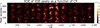 |
Fig. 2. 2D KDE analysis of the full sunspot group longitude data series, shown as a function of CR and longitude. Based on the locations of KDE peaks from the 1D KDE constructed from individual CRs. The colour scale indicates the probability density, with brighter regions corresponding to higher concentrations of activity, and thus potential ALs. |
The longitudinal distribution of each solar cycle was also examined separately using individual 2D KDEs with optimised bandwidths, set to 0.15 for both sunspot and flare datasets. For example, in the cases of Solar Cycles 19 and 23 (Figs. 3 and 4), multiple ALs are apparent, although each cycle exhibits a dominant one (the brightest region). For Solar Cycle 19, the strongest ∼50-degree-wide AL appears around CR 1415, centred at approximately 280°. Meanwhile, for Solar Cycle 23, the primary ∼30-degree-wide AL is located around CR 2010, centred at approximately 80°.
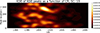 |
Fig. 3. Similar to Fig. 2 but showing the 2D KDE of sunspot group longitudes for Solar Cycle 19 only. |
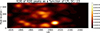
Similar to sunspots, the most populated longitudes for energetic flares were identified between Solar Cycles 17 and 24, as well as including Cycle 25 up to the summer of 2024. These were determined using individual 2D KDEs with optimised bandwidths of 0.15, as in the case of sunspot groups. Energetic flares tend to occur at preferred longitudes, similar to the distribution observed for sunspots, as is shown in Fig. 5. However, it is important to note that the flare dataset is much smaller compared to that of the sunspots.
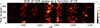 |
Fig. 5. 2D KDE analysis of the full flare longitude data series, shown as a function of CR and longitude, as in Fig. 2. |
The longitudinal distribution of flares in each solar cycle was also investigated separately. For example, in Solar Cycle 19, as shown in Fig. 6, the KDE identified the most favourable longitudes around 0° and 280°, with these regions remaining dominant throughout the cycle. In particular, the 280° longitude was also identified as a preferred location for sunspots during this cycle. In the case of Solar Cycle 23 (Fig. 7), the most dominant longitude for flares was found around 80°, corresponding to the preferred location for sunspots. However, an additional prominent longitude was also identified around 250°, approximately 180° away. This alignment is consistent with the hypothesis that ALs often exhibit a counterpart located approximately 180° apart (Elek et al. 2024).
The actual values of the measured ALs in Fig. 2 (sunspots) and Fig. 5 (flares) can be found in Table A.1. The table provides the determined longitudes of the centres of the ALs detected in sunspot groups and solar flares, along with their widths, central CRs, and durations in CR. Additionally, the averages, standard deviations, and medians of the ALs’ sizes and durations are also listed. On average, sunspot-based ALs persisted for approximately 25 CRs and had an average width of about 40°. For flare data, the average lifetime of ALs was shorter, around 15 CRs, although their average width remained similar at about 40°. However, there are both longer- and shorter-lived, as well as wider and narrower, ALs.
Based on the properties of the identified ALs described in Table A.1 and shown in Figs. 2–7, we were able to identify the presence of a flip–flop pattern in the evolution of ALs. In this pattern, one AL fades while a new one emerges, typically more than 100° apart. For example, Table A.1 shows that SC12 hosts several ALs in succession: an AL around 100° at CR 370, followed by an AL at 300° at CR 395, then at 120° at CR 410, and finally at 230° around CR 415.
Furthermore, we highlight cases where subsequent ALs appear close to each other in time, such as during Solar Cycle 18, when two ALs were identified at 260° and 270° longitude at CR 1250 and 1310, respectively. These may represent a single migrating AL, gradually shifting due to solar differential rotation. This observation underscores the fact that differential rotation remains influential, even when analysing data in the Carrington co-ordinate system. The observed flip–flop behaviour and migration of ALs are in good agreement with earlier findings by Berdyugina & Usoskin (2003) and Gyenge et al. (2014).
3.2. Testing the concept of active longitudes based on synthetic sunspot data
The question of whether these structures could be explained by the prevailing theory that sunspot groups appear with a uniform longitudinal distribution naturally arises. In this subsection we investigate this hypothesis by simulating sunspot group data with randomised parameters, focusing primarily on longitude and size, as these properties were used in the previous analyses. We applied the same analysis method, described earlier, to the simulated data as a next step, to identify any differences or similarities. Subsequently, we examined the number of KDE peaks found per number of CRs to argue that the observed longitudinal distribution of sunspot groups is inconsistent with a purely random distribution.
First, we conducted test simulations for two different cases using random number generators:
-
Phases: A case in which the occurrence and sizes of sunspot groups follow the phase of the solar cycle, as is shown in Fig. 8. The example presented corresponds to this scenario.
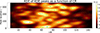
Fig. 8. Artificially generated solar cycle, after KDE analysis.
-
Phases + Long Lives: Building on the previous case, some sunspot groups are allowed to have longer lifetimes spanning several CRs. This is achieved following the Gnevyshev-Waldmeier rule, which establishes a linear relationship between sunspot group sizes and their lifetimes (Waldmeier 1955). Since we work with synoptic maps, shorter-lived spots do not significantly affect our study, as these are not captured precisely by the rule (Petrovay & van Driel-Gesztelyi 1997) and would only appear on one CR’s map in any case.
The random data generator utilises the previously constructed synoptic maps as a reference to estimate the number of CRs per cycle, the number of sunspots, and their sizes. We employed Python’s numpy module to generate appropriate distributions for each parameter. As a first step, Gaussian distributions were used to simulate the length of a solar cycle and the total number of sunspots during a cycle. A solar cycle was modelled with an average length of 145 CRs and a standard deviation of 10 CRs. Similarly, the total number of sunspots per cycle was simulated with a mean of 1200 and a standard deviation of 200, in the phases case. In the long-lived AL scenario, we used a mean of 1000 sunspots with a standard deviation of 150. This approach ensured that the total number of data points in the synoptic maps remained consistent with the original case, in which individual sunspot groups could not appear multiple times in the same synoptic map.
As the next step, a triangular distribution was adopted as a simplified model to represent the number of sunspot groups per CR throughout the rising, maximum, and declining phases of a solar cycle. More specifically, the centre of the distribution was chosen from a normal distribution with a mean of 0.375 times the cycle length and a standard deviation of 0.08 times the cycle length, to reflect the three observed phases (rising, maximum, and declining) in real solar cycle data. The total number of points in the triangular distribution corresponded to the number of sunspots in the cycle, while its total span matched the generated cycle length in CRs. The sizes of the sunspot groups were modelled using an exponentially decreasing distribution, reflecting trends observed in histograms of real observational data (Korsós et al. 2013). To simulate the typical solar cycle behaviour, the parameter of the np.random.exponential function was defined as a function of the CR to resemble a sinusoidal peak. Specifically, it was defined as: ![Mathematical equation: $ 100 \cdot \sin\left(\frac{\pi}{2} \cdot \left[\text{ CR of spot group} / \text{ length of cycle}\right]\right) $](/articles/aa/full_html/2026/03/aa56599-25/aa56599-25-eq1.gif) . Finally, each sunspot group was assigned a random longitude, drawn from a uniform distribution between 0° and 360°, to simulate their spread across the solar disc.
. Finally, each sunspot group was assigned a random longitude, drawn from a uniform distribution between 0° and 360°, to simulate their spread across the solar disc.
The same analysis steps as were used with the actual data were then applied to this simulated synthetic data. The resulting 2D KDEs display a markedly different structure, characterised by more frequent simultaneous bright areas and significantly fewer voids than in the observed data. In addition, the found ALs of the simulated data appear much narrower than in the observed data. For instance, as is illustrated in Fig. 8, we can observe a different structure than those in Figs. 3 or 4. This discrepancy provides a possible, albeit challenging to quantify, indication that the observed ALs of sunspot groups may not be random.
Let us now introduce the number of KDE peaks per CR within a solar cycle, i.e. the peaks per Carrington rotation (PPC), essentially to estimate the average number of KDE peaks per CR for each cycle, as a potentially better indicator. For these two cases, we ran our code for 10 000 solar cycles, calculating the PPC for each cycle. The resulting distributions of the PPC can be seen in the upper panels of Fig. 9, alongside the PPC distribution obtained from the observed sunspot group dataset. Intuitively, it appears unlikely that the distribution represented by the 13 consecutive observed cycles could have originated from the distributions generated by a random uniform distribution of sunspot longitudes.
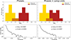 |
Fig. 9. Upper panels: histograms of the # of 1D KDE peaks found per CR for the measured sunspot data and samples from randomly generated solar cycles for two cases. Solar cycles have an increasing and a decreasing phase of activity, and sunspots can live up to multiple CRs. The randomised data are of 13 cycles randomly chosen from our samples for each case. Bottom panels: Histograms of the Cucconi test p values for 10 000 groups of 13 randomly sampled solar cycles from the random numbers generator, corresponding to the cases of the upper panels. |
To quantify this intuition, we performed Cucconi tests, as this test has been shown to yield reliable results even for relatively small sample sizes (Marozzi 2009). The Cucconi test4, using the cucconi.test and cucconi.teststat functions, with p values computed through cucconi.dist.perm, all translated into Python code for our uses from the original R, was applied. For an appropriate comparison, 13 random cycles were selected from each of the two proposed scenarios (Phases and Phases + Long Lives). Then, p values were computed for these tests, and the tests were repeated for 10 000 samples of 13 artificial cycles. The resulting distributions of p values can be seen in the bottom panels of Fig. 9, alongside average and median values of the different p values. The scenario most relevant is the Phases + Long Lives one, as this has sunspots that survive more than one CR, through a realistic relationship of lifetime with sunspot group size. The average p value here is 0.0151, meaning it is unlikely that the sunspot groups appear in random longitudes. Alternatively, if we use the median, the value is even lower, at 0.0097. Overall, this leads us to deduce that there might a physical process at work here, resulting in the distributions difficult to reconcile with a longitude-independent Sun.
4. Summary and conclusions
A number of studies have shown that solar activity on the Sun is not randomly distributed over heliographic longitude. Instead, they tend to appear more frequently in certain longitudinal intervals. These concentrations have been described by various terms, such as hearths of sunspots (Becker 1955), activity nests (Castenmiller et al. 1986), activity complexes (Gaizauskas et al. 1983; Bumba & Howard 1965), hot spots (Bai 1988), and ALs (Berdyugina & Usoskin 2003; Obridko 2010; Gyenge et al. 2016; Elek et al. 2024; Korsós & Erdélyi 2025, and references therein). Despite the differing terminology, datasets (e.g. sunspot records, synoptic maps, solar eruptions, solar faculae), and analytical techniques used, ranging across several solar cycles, these studies consistently support the clustering nature of solar activity in longitude over extended timescales.
In our study, our aim has also been to investigate whether sunspots and large energetic flares exhibit clustering along the same or not the same longitudinal direction. To do this, we utilised the sunspot group catalogue compiled by Mandal et al. (2020), which covers Solar Cycles 12–24. For flare data, we utilised H-alpha flares from the SOON catalogue and X-ray flares from GOES, both encompassing Solar Cycles 18–24. After generating Carrington maps, we extracted the longitudinal co-ordinates of sunspot groups and flares and applied 1D and 2D KDE to highlight regions of concentrated activity. The 1D KDE identifies where activity tends to cluster in longitude, while the 2D KDE reveals how these patterns evolve over time in the longitude–CR domain.
Our analysis revealed that both sunspots and flares exhibit clear clustering in longitude, namely around AL. We found that during each solar cycle, ALs vary in both lifetime and spatial extent – some persist for longer or shorter periods, and some are wider or narrower. More specifically, the longitudinal plots (Figs. 2–7) consistently reveal regions of enhanced (brighter) and reduced (darker) activity. The horizontal structures observed suggest that certain longitudes tend to remain active over extended periods, while darker regions correspond to longitudes with lower sunspot activity. These results highlight the presence of longitudinal clustering in sunspot group emergence over time and provide evidence of the existence of preferred longitudes (ALs) throughout Solar Cycles 11–24. Although the exact locations of sunspot groups and flares do not always coincide, notable structural similarities are visible across both datasets. For example, during Solar Cycle 23, both flares and sunspots exhibit a pronounced region of enhanced activity near CR 1980 at approximately 200° longitude, along with arc-like structures extending from 0° to 100° longitude.
In general, sunspot-based ALs persisted for about 25 CRs, with a typical width of about 40° (see median value in Table A.1). In comparison, flare-based ALs had shorter lifetimes of around 15 CRs, but similar widths of about 40°. These measured widths are consistent with previous findings, which report ALs ranging from 20° to 60° (Bai 1988, 2003; Bumba & Howard 1969; Gyenge et al. 2016). However, the sunspot-based lifetimes observed here are somewhat longer than the 10–15 CR range commonly cited in the literature (e.g. Elek et al. 2024). This difference in duration may reflect the fact that not all ARs situated along ALs produce major flares, as has been shown by Korsós & Erdélyi (2025). Only magnetically complex ARs – which require time to develop – are capable of generating significant solar eruptions. Consequently, flare-based ALs may appear more sporadically and for shorter periods. These results strongly suggest that as-yet-unknown, and therefore unexplored, physical mechanisms may be influencing the formation and persistence of ALs. Based on Table A.1 and in Figs. 2–7, we also observed flip–flop behaviour and the migration of ALs driven by differential rotation, in good agreement with earlier findings by Berdyugina & Usoskin (2003) and Gyenge et al. (2014).
To test whether the observed clustering around AL could result from a random longitudinal distribution of sunspot groups, we generated synthetic sunspot datasets based on the observed synoptic maps. Key parameters such as the number of CRs per cycle, the total number of sunspots, and their sizes were drawn from realistic distributions (Gaussian, triangular, and exponential). Sunspot longitudes were randomly assigned. This simulation was repeated 10 000 times across 13 synthetic cycles, corresponding to the 13 full solar cycles available in our dataset. For each cycle, we determined the number of PPCs in the KDE profiles. The resulting PPC distributions for the synthetic datasets are shown in the upper panels of Fig. 9, alongside the PPC distribution derived from the real sunspot group data. We found that the PPC distribution for the observed data differs significantly from those generated using randomised synthetic longitudes. Cucconi tests confirmed that these distributions are statistically distinct, with p values around 0.016, indicating a strong level of confidence that the observed longitudinal clustering is not due to chance.
Our findings here suggest the necessity of a more advanced solar dynamo model, one that is 3D and capable of accounting for both the observed longitudinal and latitudinal evolutions of solar activity proxies. Such a model can incorporate the concept of ALs (Usoskin et al. 2007; Berdyugina et al. 2006) or potentially utilise a two-dynamo framework to account for the spatial patterns identified in this study.
Acknowledgments
We would like to thank the referee for their valuable comments and suggestions, which helped us improve the manuscript. K.Cs. is thankful for the Eötvös Loránd University’s PhD fellowship program. M.B.K is grateful for the Leverhulme Trust Found ECF-2023-271. Sz.S. acknowledges the support (grant No. C1791784) provided by the Ministry of Culture and Innovation of Hungary of the National Research, Development and Innovation Fund (NKFIH) financed under the KDP-2021 funding scheme. R.E. is grateful to Science and Technology Facilities Council (STFC, grant No. ST/M000826/1) UK and acknowledges PIFI (China, grant number No. 2024PVA0043) for enabling this research. M.B.K, Sz.S and R.E. acknowledge the support received from NKFIH OTKA (grant No. K142987) and the Institutional Excellence Programme (grant nr TKP2021-NKTA-64), Hungary. This work was also supported by the International Space Science Institute project (ISSI-BJ ID 24-604) on Small-scale eruptions in the Sun.
References
- Bai, T. 1988, ApJ, 328, 860 [NASA ADS] [CrossRef] [Google Scholar]
- Bai, T. 2003, ApJ, 585, 1114 [NASA ADS] [CrossRef] [Google Scholar]
- Becker, U. 1955, Z. Astrophys., 37, 47 [Google Scholar]
- Benevolenskaya, E. E., Kosovichev, A. G., & Scherrer, P. H. 1999, Sol. Phys., 190, 145 [Google Scholar]
- Benz, A. O. 2008, Liv. Rev. Sol. Phys., 5, 1 [Google Scholar]
- Benz, A. O. 2017, Liv. Rev. Sol. Phys., 14, 2 [Google Scholar]
- Berdyugina, S. V., & Usoskin, I. G. 2003, A&A, 405, 1121 [NASA ADS] [CrossRef] [EDP Sciences] [Google Scholar]
- Berdyugina, S. V., Moss, D., Sokoloff, D., & Usoskin, I. G. 2006, A&A, 445, 703 [NASA ADS] [CrossRef] [EDP Sciences] [Google Scholar]
- Bhatnagar, A., & Livingston, W. 2005, Fundamentals of Solar Astronomy (World Scientific) [Google Scholar]
- Bogart, R. S. 1982, Sol. Phys., 76, 155 [NASA ADS] [CrossRef] [Google Scholar]
- Bumba, V., & Howard, R. 1965, ApJ, 141, 1502 [NASA ADS] [CrossRef] [Google Scholar]
- Bumba, V., & Howard, R. 1969, Sol. Phys., 7, 28 [Google Scholar]
- Bumba, V., Garcia, A., & Klvaňa, M. 2000, Sol. Phys., 196, 403 [NASA ADS] [CrossRef] [Google Scholar]
- Buzulukova, N., & Tsurutani, B. 2022, Front. Astron. Space Sci., 9, 429 [NASA ADS] [CrossRef] [Google Scholar]
- Canfield, R. C., & Pevtsov, A. A. 1998, ASP Conf. Ser., 140, 131 [NASA ADS] [Google Scholar]
- Castenmiller, M. J. M., Zwaan, C., & van der Zalm, E. B. J. 1986, Sol. Phys., 105, 237 [CrossRef] [Google Scholar]
- Elek, A., Korsós, M., Dikpati, M., et al. 2024, ApJ, 964, 112 [Google Scholar]
- Gaizauskas, V., Harvey, K. L., Harvey, J. W., & Zwaan, C. 1983, ApJ, 265, 1056 [NASA ADS] [CrossRef] [Google Scholar]
- Gyenge, N., Baranyi, T., & Ludmány, A. 2014, Sol. Phys., 289, 579 [Google Scholar]
- Gyenge, N., Ludmány, A., & Baranyi, T. 2016, ApJ, 818, 127 [NASA ADS] [CrossRef] [Google Scholar]
- Hathaway, D. H. 2015, Liv. Rev. Sol. Phys., 12, 4 [Google Scholar]
- Korsós, M. B., & Erdélyi, R. 2025, ApJ, 989, 162 [Google Scholar]
- Korsós, M. B., Baranyi, T., & Ludmány, A. 2013, Cent. Eur. Astrophys. Bull., 37, 425 [Google Scholar]
- Korsós, M. B., Elek, A., Zuccarello, F., & Erdélyi, R. 2024, ApJ, 975, 248 [Google Scholar]
- Losh, H. M. 1939, Publications of Michigan Observatory, 7, 127 [NASA ADS] [Google Scholar]
- Mandal, S., Krivova, N. A., Solanki, S. K., Sinha, N., & Banerjee, D. 2020, A&A, 640, A78 [NASA ADS] [CrossRef] [EDP Sciences] [Google Scholar]
- Marozzi, M. 2009, J. Nonparametric Stat., 21, 629 [Google Scholar]
- Mugatwala, R., Chierichini, S., Francisco, G., et al. 2024, J. Space Weather Space Clim., 14, 6 [Google Scholar]
- Mursula, K., & Hiltula, T. 2004, in 35th COSPAR Scientific Assembly, 35, 2817 [Google Scholar]
- Obridko, V. N. 2010, IAU Symp., 264, 241 [Google Scholar]
- Parzen, E. 1962, Ann. Math. Stat., 33, 1065 [Google Scholar]
- Petrovay, K., & van Driel-Gesztelyi, L. 1997, Sol. Phys., 176, 249 [Google Scholar]
- Pevtsov, A. A., & Balasubramaniam, K. S. 2003, Adv. Space Res., 32, 1867 [NASA ADS] [CrossRef] [Google Scholar]
- Pevtsov, A. A., & Canfield, R. C. 1999, Geophysical Monograph Series, 111, 103 [Google Scholar]
- Pevtsov, A. A., & Canfield, R. C. 2000, J. Astrophys. Astron., 21, 185 [Google Scholar]
- Rosenblatt, M. 1956, Ann. Math. Stat., 27, 832 [Google Scholar]
- Ruzmaikin, A., Feynman, J., Neugebauer, M., & Smith, E. J. 2001, J. Geophys. Res., 106, 8363 [Google Scholar]
- Schrijver, C. J. 2009, Adv. Space Res., 43, 739 [NASA ADS] [CrossRef] [Google Scholar]
- Tian, L., Bao, S., Zhang, H., & Wang, H. 2001, A&A, 374, 294 [NASA ADS] [CrossRef] [EDP Sciences] [Google Scholar]
- Tian, Y. 2022, J. Phys.: Conf. Ser., 2282, 012025 [Google Scholar]
- Toriumi, S., Schrijver, C. J., Harra, L. K., Hudson, H., & Nagashima, K. 2017, ApJ, 834, 56 [Google Scholar]
- Usoskin, I., Berdyugina, S., Moss, D., & Sokoloff, D. 2007, Adv. Space Res., 40, 951 [NASA ADS] [CrossRef] [Google Scholar]
- Vourlidas, A., Patsourakos, S., & Savani, N. P. 2019, Phil. Trans. Royal Soc. London Ser. A, 377, 20180096 [Google Scholar]
- Waldmeier, M. 1955, Ergebnisse und Probleme der Sonnenforschung (Geest& Portig) [Google Scholar]
- Wang, Y., & Zhang, J. 2008, ApJ, 680, 1516 [Google Scholar]
- Zhang, H., & Bao, S. 1999, ApJ, 519, 876 [Google Scholar]
- Zhang, L., Mursula, K., Usoskin, I., & Wang, H. 2011, A&A, 529, A23 [NASA ADS] [CrossRef] [EDP Sciences] [Google Scholar]
Appendix A: Table of active longitudes
Measured properties of the ALs identified in the sunspot group and flare datasets.
All Tables
Measured properties of the ALs identified in the sunspot group and flare datasets.
All Figures
|
Fig. 1. Ridge plot showing the longitudinal distribution of sunspot group activity during the year 1956. Each strip represents a single CR within the year. Note that they do not necessarily begin or end in that year. The x axis shows Carrington longitude within the individual CRs shown, while the y axis is proportional to the probability density determined by the KDE. |
| In the text | |
|
Fig. 2. 2D KDE analysis of the full sunspot group longitude data series, shown as a function of CR and longitude. Based on the locations of KDE peaks from the 1D KDE constructed from individual CRs. The colour scale indicates the probability density, with brighter regions corresponding to higher concentrations of activity, and thus potential ALs. |
| In the text | |
|
Fig. 3. Similar to Fig. 2 but showing the 2D KDE of sunspot group longitudes for Solar Cycle 19 only. |
| In the text | |
|
Fig. 5. 2D KDE analysis of the full flare longitude data series, shown as a function of CR and longitude, as in Fig. 2. |
| In the text | |
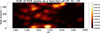 |
Fig. 6. Similar to Fig. 5, but shows the 2D KDE of energetic flares longitudes for Solar Cycle 19. |
| In the text | |
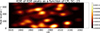 |
Fig. 7. Same as Fig. 5 but for Solar Cycle 23. |
| In the text | |
|
Fig. 8. Artificially generated solar cycle, after KDE analysis. |
| In the text | |
|
Fig. 9. Upper panels: histograms of the # of 1D KDE peaks found per CR for the measured sunspot data and samples from randomly generated solar cycles for two cases. Solar cycles have an increasing and a decreasing phase of activity, and sunspots can live up to multiple CRs. The randomised data are of 13 cycles randomly chosen from our samples for each case. Bottom panels: Histograms of the Cucconi test p values for 10 000 groups of 13 randomly sampled solar cycles from the random numbers generator, corresponding to the cases of the upper panels. |
| In the text | |
Current usage metrics show cumulative count of Article Views (full-text article views including HTML views, PDF and ePub downloads, according to the available data) and Abstracts Views on Vision4Press platform.
Data correspond to usage on the plateform after 2015. The current usage metrics is available 48-96 hours after online publication and is updated daily on week days.
Initial download of the metrics may take a while.