| Issue |
A&A
Volume 707, March 2026
|
|
|---|---|---|
| Article Number | A245 | |
| Number of page(s) | 13 | |
| Section | Numerical methods and codes | |
| DOI | https://doi.org/10.1051/0004-6361/202556662 | |
| Published online | 17 March 2026 | |
A semi-coherent search for optical pulsations from Scorpius X-1
1
INAF – Osservatorio Astronomico di Roma,
Via Frascati 33,
00078
Monte Porzio Catone,
Italy
2
INAF – Osservatorio Astronomico di Brera,
Via Bianchi 46,
23807
Merate (LC),
Italy
3
INFN, Sezione di Roma,
00185
Roma,
Italy
4
Università di Roma ‘La Sapienza’,
00185
Roma,
Italy
5
University of Oxford, Department of Physics, Astrophysics,
Keble Road,
Oxford
OX1 3RH,
UK
6
Fundación Galileo Galilei - INAF,
Rambla J.A. Fernández P. 7,
38712
B. Baja (S.C. Tenerife),
Spain
7
Dipartimento di Fisica e Astronomia, Sezione Astrofisica, Università di Catania,
Via S. Sofia 78,
95123
Catania,
Italy
8
INAF – Osservatorio Astrofisico di Catania,
Via S. Sofia 78,
95123
Catania,
Italy
★ Corresponding author: This email address is being protected from spambots. You need JavaScript enabled to view it.
Received:
30
July
2025
Accepted:
18
January
2026
Abstract
The emission of continuous gravitational waves (CWs) possibly explains why pulsars spinning with a period shorter than a millisecond have not been observed so far. Neutron stars accreting mass at the highest rates are the most promising targets for a search for CWs, because a strong emission of gravitational waves is required to balance the torque exerted by mass accretion onto the neutron star. Detecting coherent pulsations in the electromagnetic emission maximizes the search sensitivity, but has so far not been successful for most of the brightest accreting neutron stars. Here, we present the first search for pulsations in the optical band from the brightest accreting neutron star known, Sco X-1. To this end, we tailored semi-coherent search strategies to data obtained over four years, for a total of ~56 ks, by the SiFAP2 fast photometer mounted at the Telescopio Nazionale Galileo (TNG). These searches are especially suited to analysing long observations of systems for which only limited knowledge on the orbital parameters is available, and involve joining coherent analyses on shorter segments without connecting the spin phase between them. The large count rates afforded by an optical telescope and the efficiency of the search strategy employed allowed us to set an upper limit of 9 × 10⁻⁵ to the pulsed amplitude, which is lower by a factor of four with respect to previous searches in the X-ray band. We also show that the application of semi-coherent searches to SiFAP2 observations of the first detected optical millisecond pulsar, PSR J1023+0038, could have preceded its detection in the radio band. These results highlight the role played by high-time-resolution optical observations in performing deep searches of quickly rotating pulsars.
Key words: techniques: photometric / binaries: general / pulsars: general / X-rays: individuals: Scorpius X-1
© The Authors 2026
 Open Access article, published by EDP Sciences, under the terms of the Creative Commons Attribution License (https://creativecommons.org/licenses/by/4.0), which permits unrestricted use, distribution, and reproduction in any medium, provided the original work is properly cited.
This article is published in open access under the Subscribe to Open model. This email address is being protected from spambots. You need JavaScript enabled to view it. to support open access publication.
1 Introduction
Accretion of mass and angular momentum transferred from a low-mass companion star in a binary system can spin a neutron star (NS) up to a rotational frequency of hundreds of hertz. Soon after the discovery of rotation-powered millisecond pulsars (MSPs; Backer et al. 1982), low-mass X-ray binaries (LMXBs) were proposed as their progenitors (Alpar et al. 1982; Radhakrishnan & Srinivasan 1982). Accreting X-ray millisecond pulsars in transient LMXBs (Patruno & Watts 2021; Di Salvo & Sanna 2022) demonstrated that disc accretion can actually spin up a NS to such periods (Bisnovatyi-Kogan & Komberg 1976; Wijnands & van der Klis 1998). Observations of transitions between accretion- and rotation-powered emission on timescales of less than a few days eventually proved the evolutionary link between these two classes of NS (Archibald et al. 2009; Papitto et al. 2013; Bassa et al. 2014; Papitto & de Martino 2022).
Keplerian break-up limits the maximum spin of a NS at ~1 kHz or above, depending on the equation of state describing the rotating compact object (Cook et al. 1994; Lattimer & Prakash 2007). In principle, detecting a very fast, sub-millisecond spinning NS would immediately rule out some of the proposed models (see e.g. Bhattacharyya et al. 2016, and references therein). However, the observed distribution of spin frequencies of MSPs sharply cuts off at ~700 Hz (Chakrabarty et al. 2003; Chakrabarty 2008; Hessels 2008; Papitto et al. 2014; Patruno et al. 2017). The strongly frequency-dependent spindown torque related to the emission of continuous gravitational waves (CWs) might explain the lack of very quickly spinning NSs (Bildsten 1998; Andersson et al. 2005): elastic and/or magnetic deformations of the distribution of the accreted matter onto the NS surface, instabilities from bar-mode and r-mode oscillations, and free precession are some of the mechanisms proposed to drive off a NS from axis-symmetry and emit CWs (see Sieniawska & Bejger 2019 and references therein). Besides selection effects, alternative models to explain the lack of submillisecond pulsars include magneto-dipole rotation and/or propeller spin down occurring when the secular mass-accretion phase ends altogether (Burderi et al. 2001; Tauris 2012) or when it decreases during the quiescent phases of X-ray transients (Stella et al. 1994; Bhattacharyya & Chakrabarty 2017), and standard magnetic disc accretion torque theory for given values of the pulsar magnetic field and accretion rate (Andersson et al. 2005).
The possibility that CW emission might limit the spin rate of MSPs prompted several search attempts with the latest generations of GW interferometers, with no detection reported to date (see e.g. Abbott et al. 2022a,b,c,d,e; Whelan et al. 2023; Steltner et al. 2023; Abac et al. 2025). Assuming that CW emission balances the spin-up imparted to the NS by mass accretion, the brightest accreting NSs in LMXBs are widely considered the best candidates for CW detection (see Watts et al. 2008 and references therein). With an accretion rate close to matching the Eddington rate at a distance of a few kiloparsecs (Bradshaw et al. 1999, 2003; McNamara et al. 2005), Scorpius X-1 stands out in this regard. In addition, some of its orbital parameters were measured with good accuracy through optical observations (Wang et al. 2018; Killestein et al. 2023), reducing the volume of the parameter space that a coherent signal search has to investigate (see Sect. 2). However, deep searches for a coherent spin modulation at radio (Taylor et al. 1972) and X-ray energies (Wood et al. 1991 ; Ubertini et al. 1992; Vaughan et al. 1994; Galaudage et al. 2022) were not successful. This significantly hampered the sensitivity of CW searches (Abbott et al. 2007, 2019, 2022e; Zhang et al. 2021; Whelan et al. 2023; Amicucci et al. 2025), as accurate knowledge of the position in the sky, the binary parameters, and the spin frequency and its evolution is required to maximize their sensitivity.
Recently, the visible band emerged as a promising alternative channel to search for fast coherent signals from MSPs. SiFAP2 (Ghedina et al. 2018), a fast optical photometer operated from the 3.6 m Telescopio Nazionale Galileo (TNG), detected optical pulsations from a transitional (Ambrosino et al. 2017; Papitto et al. 2019; Illiano et al. 2023; see also Zampieri et al. 2019; Karpov et al. 2019), an accreting (Ambrosino et al. 2021), and a rotation-powered MSP (Papitto et al. 2025). The minimum detectable pulsed amplitude, A, depends on the number of photons in the observation, Nγ, through A ∝ N−1/2 (e.g. Wood et al. 1991; Vaughan et al. 1994). An instrument such as SiFAP2 from the TNG records around a few × 105 photons per second from a source with an apparent magnitude of V ~ 12-13 mag, such as Sco X-1 (see Table 1). As a result, searches for coherent signals in the optical band are slightly more sensitive for a given exposure time than, for example, X-ray telescopes, which in turn typically observe approximately a few × 104 photons per second, at most (see e.g. La Monaca et al. 2024), although the relative contribution from the NS expected in the X-ray band is higher than in the optical one. For the two optical MSPs that also show X-ray pulsations, SAX J1808.4-3658 and PSR J1023+0038, the pulsed fractional amplitudes in the X-ray band are approximately ten times higher than in the optical band: however, taking observations made with SiFAP2 and the PN instrument on XMM-Newton as an example, the ratio between their photon count rates in the optical and X-ray bands are ~150 and ~4000, outweighing the offset in pulsed amplitude (Ambrosino et al. 2017, 2021).
Here, we present the first search for optical pulsations from Sco X-1 using SiFAP2/TNG observations. To maximize the sensitivity, we adapted semi-coherent search techniques (see Sect. 2) to the case of optical data. Section 3 describes our algorithm, which loosely follows the one applied in Messenger & Patruno (2015), whereas in Sects. 4 and 5 we discuss the statistical properties of the combined detection statistics and the significance of both signals and upper limits. Section 6 shows a first application of the algorithm to data from a known pulsar, PSR J1023+0038, and Sect. 7 contains the analysis of 13 observations of Sco X-1 through the same method. Finally, in Sect. 8 we review our results and discuss future applications.
Summary of Sco X-1 observations with SiFAP2/TNG.
2 Coherent periodicity searches
Searching for a fast coherent signal from LMXBs requires dedicated techniques to account for the drifts in the observed signal frequency caused by the orbital motion. As a result, a periodicity search with, for example, a Fourier power density spectrum (PDS), is either limited to a ‘simple search’ on short time intervals, over which the binary frequency drift is negligible compared to the frequency resolution, or requires the preliminary correction of the photons’ detection times for the periodic variation of the travel time at different phases during the orbit. While the sensitivity of the former approach is sub-optimal due to the reduced number of photons in the time series and the coarser frequency resolution, the latter can become computationally prohibitive if the orbital parameters are not known in advance with a good level of precision. The cost of a ‘blind search’ by trial and error on a fine grid of possible combinations of orbital parameters scales with the length of the time interval coherently analysed as  1. In addition, the minimum detectable amplitude scales with the number of trials as
  (e.g. Wood et al. 1991; Vaughan et al. 1994). ‘Acceleration’ and ‘jerk searches’ approximate the frequency drifts caused by the orbital motion over intervals short enough with respect to the binary period with a polynomial (Hertz et al. 1990; Johnston & Kulkarni 1991; Wood et al. 1991; Bagchi et al. 2013; Andersen & Ransom 2018). As a result, they maintain the signal coherence over longer segments than simple searches, attaining greater sensitivity. However, these searches still analyse each segment separately. Sideband searches represent an alternative approach to studying observations that are longer than the orbital period, complementarily to acceleration searches (Ransom et al. 2003). They exploit the fact that orbital motion produces sidebands in the PDS around the spin frequency of the pulsar with a spacing equal to Tobs/Porb, which can be then used to correct for the orbital modulation.
To make the best possible use of large datasets which span a time interval much longer than the binary period and obviate the enormous computational costs associated with the search of weak CW signals from systems with large parameter uncertainties, Messenger (2011) proposed to use ‘semi-coherent searches’. This strategy was developed to search for CWs from isolated NSs (Brady & Creighton 2000) and has since been widely applied in searches focused on binary systems (Pletsch & Allen 2009; Astone et al. 2014; Leaci & Prix 2015; Abbott et al. 2017; Dergachev & Papa 2019; Wette 2023). It involves a coherent analysis of separate segments of a long observation and the incoherent sum of their detection statistics, keeping track of the signal orbital evolution. Here, by ‘incoherent’ we mean that information on the signal phase is lost between segments. Although less sensitive than fully coherent blind searches performed on the same observation, these techniques are computationally much more efficient, so that at fixed computational cost they permit us to search larger portions of the parameter space or reach higher sensitivities (e.g. Prix & Shaltev 2012). Similar to the case of CWs, searching for binary gamma-ray pulsars relies on year-long data integration and naturally implemented semi-coherent strategies, yielding some detections in recent years (Pletsch et al. 2012; Nieder et al. 2020b; Clark et al. 2021). The method from Messenger (2011) was also applied four times to X-ray data of LMXBs (Messenger & Patruno 2015; van den Eijnden et al. 2018; Patruno et al. 2018; Galaudage et al. 2022).
In the next section, we describe in full the semi-coherent algorithm we adopted to analyse high-photon-count-rate datasets observed in the optical band.
3 Method
In the case of a NS in a binary system, any periodic signal at the spin frequency, f, is observed as modulated by the Doppler shift due to the projected velocity of the pulsar. Assuming a circular orbit, the detection time t of a photon emitted at a given time τ is, after correcting for our position relative to the Solar System barycentre,
![Mathematical equation: t = \tau + \frac{a_1\sin(i)}{c} \ \sin \left[ \frac{2 \pi}{P_{\mathrm{orb}}} (\tau -T_{\mathrm{asc}}) \right] + \frac{d}{c} ,](/articles/aa/full_html/2026/03/aa56662-25/aa56662-25-eq3.png) (1)
(1)
where a1 sin(i)/c = a⊥ is the projected semi-major axis of the NS orbit around the binary’s centre of mass, Porb is the orbital period, Tasc is the time at which the NS crosses the ascending node during its orbit, and d is the binary’s distance from the Solar System. The observed frequency of the signal is
![Mathematical equation: \nu_{\mathrm{obs}}(t) = f \left(1 - a_\perp \Omega \cos{\left[ \Omega(t-T_{\mathrm{asc}}) \right]} \right) ,](/articles/aa/full_html/2026/03/aa56662-25/aa56662-25-eq4.png) (2)
(2)
where we introduced Ω = 2π/Porb to simplify the notation. Therefore, in the PDS the signal can be spread across all the frequency bins that go from the minimum to the maximum of νobs(t) across an orbit.
To take into account this frequency drift while keeping the problem computationally tractable, Messenger (2011) proposed to divide the process into two steps. First, a coherent pulsation search is performed on M separate segments of length Tseg out of a Tspan-long observation (the coherent step). Then, each orbital parameter combination of interest is explored by summing the powers found in different segments during the coherent step, at the frequencies produced by the signal modulation according to Eq. (2) (the semi-coherent step).
3.1 The coherent step
In the following, we always consider segments that are short compared to the orbital period of the source. In each segment m, we can approximate the observed frequency of the signal by Taylor-expanding Eq. (2) to the s*-th order (Messenger 2011; Messenger & Patruno 2015, after correcting one sign):
 (3)
(3)
where tm is the mid-point of the segment,
![Mathematical equation: \nu_{s}^{(m)} = \left\{ \begin{array}{cr} f \left(1 - a_\perp \Omega \cos{\left[\gamma^{(m)}\right]} \right) \qquad &\text{for } s=1 \\ -f a_\perp \Omega^s \sin{\left[\gamma^{(m)} + s\frac{\pi}{2} \right]} \qquad &\text{for } s>1 \end{array} \right.](/articles/aa/full_html/2026/03/aa56662-25/aa56662-25-eq6.png) (4)
(4)
and  . Similarly, the time correction from each PTA in the segment,
  , to its related emission time at the NS can be approximated through
 (5)
(5)
The uncertainty range in Ω and a⊥ sets the range spanned by the various  (see Eq. (4)), i.e. the boundaries of each dimension of the coherent space. Then, we populated our coherent space by placing a grid of combinations of
  for each segment, whose spacing depends on the maximum fractional loss in power, μ*, that we allowed. We can associate with any given μ* a coherent space metric, gij, which describes the distance between points in the space of vectors ν = (ν1, ν2,..., νs.) (Messenger 2011). The correct general form of the metric is found in Sect. IV C of Leaci & Prix (2015), but we are particularly interested in the diagonal terms, gjj, which are a good approximation of its general form for short segments (see Messenger 2011), and the first four terms are2
 (6)
(6)
We placed our points on hypercubic cells whose sides are then given by (Messenger & Patruno 2015)
 (7)
(7)
and in the following we always use μ* = 5%. Therefore, we define s* as the largest order for which the total range found through Eq. (4) is larger than its related spacing following Eq. (7) would be.
On each grid point of the coherent space, we corrected the photons’ detection times through Eq. (5) and create M matrices of coherent detection statistics, i.e. the power Λ(m), by calculating the Leahy-normalized PDS from the  (Leahy et al. 1983). All of the Λ(m) are saved for use in the semi-coherent step.
3.2 The semi-coherent step
Searches based on uncertain orbital parameters entail exploring a grid of possible orbital parameter combinations, which for brevity we call templates, within those uncertainties. The traditional method for the construction of such a grid requires that every point in the parameter space be ‘covered’ at least by one template, although this becomes computationally heavy as the number of dimensions, i.e. the number of parameters, increases. As was the case for the coherent space, this implies that the grid spacing must be dense enough that any point is no further than a given distance from the closest template, which is a function of the maximum acceptable loss in signal power.
We tiled the orbital parameter space following Caliandro et al. (2012), which provided exact expressions for the expected fraction of signal power recovered, ε2, for a given distance in each dimension, thus creating a lattice. We allowed for a maximum loss for each dimension equal to 1 - ε2 = 2.5%, so that, in the worst possible case where all three binary parameter, s a⊥, Porb, and Tasc, are as far as possible from the closest lattice point, we still retain ε6 ~ 92.7% of the original power. Making the same choice, if we only search over two of the binary parameters, as is the case for the analyses discussed in Sects. 6 and 7, we retain ~95% of the power.
The search for higher-frequency coherent signals requires finer grids in all of the physical parameters with respect to low-frequency ones; therefore, the analysis is split in 100-Hz wide frequency bands. For each of them, we used the minimum spacings required (δPorb, δTasc, δa⊥) across all segments at the maximum frequency of that band. The spacing in intrinsic spin frequency is taken to be the independent discrete Fourier one, 1/ Tseg.
For each template in the parameter space, i.e. each combination θ = (f, Porb, a⊥, Tasc), we can use Eqs. (3) and (4) to search for the corresponding nearest neighbour in the coherent space in each segment, hence defining a ‘track’ in the coherent space. The sum of all the related powers, Λ(m), defines the combined statistics, Σ, whose properties are discussed in Sects. 4 and 5. The full algorithm is summarized in Appendix B.
4 Significance of detections
The total detection statistic, Σ, is the sum of the powers found in the PDS of each of the segments. In the absence of a signal, and assuming pure Poissonian noise, Σ is the sum of M individual χ2 distributions with two degrees of freedom each, and therefore follows a χ2 distribution with 2M degrees of freedom. The probability, P, of obtaining a value of the summed statistic equal to or greater than Σ in a single trial in the case of noise alone is given by
 (8)
(8)
where γ, Γ, and P are the lower incomplete, complete, and regularized lower incomplete gamma functions, respectively. Here, by single trial we mean a given sum of M Leahy-normalized power spectra. The probability of obtaining at least one value of the detection statistic in the same range in the case of n trials is thus
 (9)
(9)
and, consequently, once we choose a false-alarm probability, PFA, that we are willing to accept as adequately small, the equivalent threshold in total detection statistic is given by
 (10)
(10)
where by P−1 we denote the inverse of the regularized lower incomplete gamma function, P, in Eq. (8). Strictly speaking, Eq. (9) only holds in the case of n independent values of Σ across our parameter space; since our template grid is dense in order to avoid missing possible signals, the noise realizations in templates that are close to one another could not be completely statistically independent. This can skew the probability distribution away from Eq. (9), undermining the statistical significance of signals above the threshold (see the example of Nieder et al. 2019 for the H statistic). However, as shown in Appendix C, for the χ2 noise distributions analysed in this paper this leads to the thresholds obtained through Eqs. (9) and (10) actually being at most more conservative than necessary. We therefore used them without further corrections.
In principle, different combinations of binary parameters can produce the same evolution of the observed signal in the coherent space, i.e. the same track, owing to the finitely spaced grid in the coherent space. As a result, the number of unique tracks walked during our semi-coherent step, Nwalked, can be smaller than the total number of combinations of spin and orbital parameters, Ncomb. However, only in a handful of cases was Nwalked lower than Ncomb, and the ratio Nwaiked/Ncomb was always higher than 99.9% for the analyses presented in Sects. 6 and 7. We thus considered Ncomb as a conservative upper limit on the number of statistically independent trials made in our search. However, we note that if the maximum acceptable losses in power in the two steps of the algorithm, μ* and 1 - ε, were set to very different values, the ratio Nwalked/Ncomb would drop significantly: taking Ncomb in those cases could lead to a great overestimation of the number of independent trials carried out. Since at each frequency interval we consider the spacing in both physical and coherent templates banks change, the final number of total trials is the sum of the trials in each frequency interval.
5 Upper limit determination
Should no summed power Σ be found above the detection threshold, we can place an upper limit to the signal power, Σsignal, that might have been present in the data at any chosen confidence level. A detailed study of the probability distributions in power spectra was carried out by Groth (1975), and we used the procedures and renormalization outlined in Vaughan et al. (1994), which we briefly summarize in the following, to derive upper limits both on signal power and fractional amplitude from our maximum detected power, Σmax.
The joint probability density of measuring Σmeas through the sum of M power spectra, containing a signal of power Σsignal is (Groth 1975, renormalized)
![Mathematical equation: \begin{split} p_M(\Sigma_\mathrm{meas}, \Sigma_\mathrm{signal}) & = \frac{1}{2}\left(\frac{\Sigma_\mathrm{meas}}{\Sigma_\mathrm{signal}}\right)^{\frac{M-1}{2}} \exp\left[-\frac{\Sigma_\mathrm{meas}+\Sigma_\mathrm{signal}}{2}\right] \\ & \quad \times I_{M-1}\left(\sqrt{\Sigma_\mathrm{meas}\Sigma_\mathrm{signal}}\right) , \end{split}](/articles/aa/full_html/2026/03/aa56662-25/aa56662-25-eq18.png) (11)
(11)
where Il indicates the modified Bessel function of the first kind of order l (see e.g. Olver et al. 2010). This is simply the noncentral χ2 distribution first obtained by Fisher (1928), χ′2, with 2M degrees of freedom and non-centrality parameter equal to ∑signal; therefore, Eq. (11) can be integrated providing the probability of obtaining a power up to Σmax if a signal of power Σsignal is present in the data (Johnson et al. 1995):
 (12)
(12)
Such process can be numerically inverted to obtain, for any choice of confidence level, C, the corresponding upper limit, Σul, on signal power within our observation (Vaughan et al. 1994): that is, a signal such that the probability of it producing a measured power less than or equal to Σmax is  .
.
Finally, we can express the background-subtracted upper limit on the pulse amplitude as (see e.g. Vaughan et al. 1994; Bilous & Watts 2019)
 (13)
(13)
where Nγ,tot and Nγ,bkg are the total number of photons and the ones from the background alone, respectively, from all of the summed segments, while the factor 1.61 arises from the discrete Fourier spacing, and r is the number of orbital parameters over which the search is performed.
6 Test on PSR J1023+0038
To test the algorithm, we used it to reproduce the detection of optical pulsations from SiFAP2 data of a known pulsar in a binary system, PSR J1023+0038. It was the first transitional MSP to be discovered (Archibald et al. 2009), and the first one for which pulsations were detected in the optical band (Ambrosino et al. 2017).
We chose an optical observation from the night starting on 30 January 2020 (UTC), for a total length of almost 19 ks and 427 675 147 collected photons (target plus background). All photon detection times were corrected to the Solar System barycentre with the DE405 planetary ephemeris assuming α = 10h23m47.687198s and δ = +00°38′40.84551" as source coordinates (Jaodand et al. 2016). This was done through a custom pipeline which takes into account both the geometrical R0mer delay and the relativistic Einstein and Shapiro delays from the Sun, neglecting effects due to atmosphere, parallax, and other planets, and was already successfully used in previous analyses of SiFAP2 observations (e.g., Ambrosino et al. 2017). The observation was made with the Silicon Fast Astronomical Photometer and Polarimeter (SiFAP2; Meddi et al. 2012; Ambrosino et al. 2016; Ghedina et al. 2018), currently mounted at the 3.58-metre INAF TNG (Barbieri et al. 1994) at the Roque de Los Muchachos Observatory in La Palma. Using Silicon PhotoMultipliers (SiPMs), SiFAP2 is capable of counting individual optical photons, recording their detection times with a relative time resolution of 8 ns until 2024, now lowered to 80 ps.
All SiPMs suffer from correlated noise, specifically crosstalk and afterpulsing (Klanner 2019), which induces a slightly higher normalization of the observed PDS with respect to what would be expected from Poissonian noise; this effect is of no practical consequence in the case of powerful sources, but can bring noise fluctuations closer to or slightly above detection thresholds, thus making detections of weak signals uncertain if not taken into account. In Appendix A we carry out a detailed study of this correlated noise and its impact on PDS, and we also provide two possible methods to properly include their effects during data analysis, ensuring that all the considerations in (Sects. 4 and 5 still hold. In our case, this translates to a simple renormalization of the power observed at each frequency in the coherent step by a factor of ~1/1.15.
6.1 Analysis setup
The first detection of coherent pulsations from PSR J1023+0038 was obtained in 2009 in the radio band and led to measurements of its orbital parameters being refined to exquisite precision (Archibald et al. 2009). However, to properly validate our algorithm in the same conditions of its intended use, we decided to disregard all knowledge of the system obtained after the discovery of radio pulsations. Thanks to high-quality radial-velocity curves of the secondary star, Thorstensen & Armstrong (2005) had previously already measured the orbital period to sub-second precision (0.1980959 ± 4 ∙ 10−7 days), and therefore we kept it fixed. They had also measured the radial velocity of the companion star as K2 = 268 ± 4 km/s−1 (at a 1-σ confidence level) from which the mass ratio, q, between the secondary and the primary star could be constrained to lie between ~0.04 and ~0.75 (at a 3-σ confidence level). Through a⊥ = K2 qPorb/(2πc), we obtained bounds on a⊥ between 0.093 and 1.91 s. We also left Tasc unconstrained, letting it vary over the whole orbit. We then divided the SiFAP2 observation into 147 segments, each 128 s long, and ran the algorithm searching for pulsations at frequencies between 50 and 1550 Hz.
6.2 Results
Figure 1 shows the observed maximum value of the summed power, Σ, at each frequency searched. Two outstanding peaks (Σ1 = 2119.4, Σ2 = 2116.2) lie exactly at the frequencies of the first and second harmonics of the pulsar, the first peak being found in the bin corresponding to 592.4219(39) Hz. This value agrees with that obtained by Burtovoi et al. (2020) using the known radio orbital ephemeris to correct optical data taken during those same days f = 592.42146750 ± 7 ∙ 10−8 Hz. The other two parameters in the combination corresponding to the first peak are a⊥ = 0.3433 ± 0.0068 s and Tasc = 58878.991043 ± 29 ∙ 10−6 MJD, where the uncertainties we report are each equal to half their relative step in the parameter grid. They are compatible with the respective values known from literature, a⊥ = 0.343356 s (Jaodand et al. 2016) and Tasc = 58878.9911009 ± 12 ∙ 10−7 MJD (Illiano et al. 2023).
We conclude that our semi-coherent algorithm would have been able to discover the pulsar using SiFAP2/TNG optical data alone, i.e. without making use of any previous pulse detection in the radio and in the X-ray band, and to determine its orbital parameters correctly.
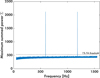 |
Fig. 1 Maximum values of the summed power Σ, regardless of the corresponding orbital parameter combination, in the 50-1550 Hz frequency range, on a SiFAP2 observation of PSR J1023+0038. The dashed black line represents the 1% false-alarm threshold, which instead is calculated for all the combinations explored. |
7 Scorpius X-1
SiFAP2 observed Sco X-1 during four campaigns that took place between 2018 and 2023, accumulating ~16 hours divided into 13 observations, and ~1.7 × 10¹⁰ photons (see Table 1). All observations were taken in white light covering the 320-900 nm band (see supplementary Fig. 1 in Ambrosino et al. 2017), except for the last observation (April 23, 2023), which was conducted with a Johnson-Bessel B passband (λeff = 445 nm, ΔλFWHM = 94 nm). We corrected the photon detection times to the Solar System barycentre with the same pipeline used for the analysis in Sect. 6, taking the source position from the Gaia catalogue: α = 16h19m55.06927s, δ = −15°38′25.01767" (Gaia Collaboration 2020). The background rates were quite different across observations, but always contributed less than 15% of the total count rate.
7.1 Analysis setup
The orbital parameters of Sco X-1 have long been monitored (starting from Gottlieb et al. 1975), and there is an ongoing programme to periodically update them especially for CW searches (Galloway et al. 2014; Wang et al. 2018; Killestein et al. 2023). The parameter that suffers from the largest uncertainties is a⊥, whose value was poorly constrained owing to the lack of precise bounds on the system’s masses: the most likely range is (1.45-3.25) s, as estimated in Wang et al. (2018). Killestein et al. (2023) measured an orbital period of Porb = (68023.92 ± 0.02) s and a time of passage at the inferior conjunction of the companion star Tcon = 2456723.3272 ± 0.0004 BJD (UTC) = 56722.8272 ± 0.0004 MJD3. We then obtained a starting value of Tasc,oid = Tcon - Porb/4 = (56722.8272 - 68023.92/86400/4) MJD ± 33 s = 56722.6304 MJD ± 33 s for the epoch of passage of the compact object at the ascending node of the orbit. We extrapolated the value of Tasc closest to each of our observations as
 (14)
(14)
and their uncertainties through the usual addition in quadrature, giving
 (15)
(15)
where ⌊∙⌋ indicates rounding to the nearest integer and MJDREFi is the reference time of each observation; we used three times the 1-σ uncertainty for both parameters. Considering these parameter ranges, we decided to take 512-s long segments to balance the load on our hardware and the amplitude we expected to reach with Sco X-1's count rate (see Eq. (13)).
Among the strengths of semi-coherent searches is the possibility to jointly analyse observations quite far removed from one another, although this implicitly assumes a sufficient stability in the system’s orbital configuration among observations. If present, a derivative on the orbital period, Ṗorb, would translate into a change in Tasc as well. The value of Ṗorb can be estimated through (see e.g. di Salvo et al. 2008)
 (16)
(16)
where g(β, q,α) = 1 -βq - (1 -β)(α + q/3)/(1 + q),β is the fraction of the mass lost by the companion star that accretes onto the NS, q = M2/M1 is the mass ratio between the companion and the NS, and J/Jorb represents possible losses of angular momentum from the system.
Supposing J to be caused by GW emission and assuming conservative mass transfer, the expected maximum Porb can be estimated by taking the smaller of the two terms in Eq. (16) to be zero. Here,  , while
  (at the 95% c.l.; Wang et al. 2018). We see that the dominant term is -Ṁ2/M2, and, assuming that J̇/Jorb = 0,
 (17)
(17)
The corresponding shift in Tasc is (e.g. Papitto et al. 2005)
 (18)
(18)
which in our case gives  s. Since the smallest value of δTasc,i across our observations is ~11.4 s, we decided to perform our searches by joining the observations of subsequent years into two datasets, 2018-2019 (D1) and 2022-2023 (D2), obtaining 51 and 58 segments, respectively.
Given this value of Tseg and the other uncertainties of the parameters, the step in Porb would be greater than its 3-σ c.l. uncertainties at all frequencies. Therefore, we only searched over a⊥ and Tasc. The first half of Table 2 summarizes the parameter ranges searched for both datasets, together with the conservative total number of trials, which is the sum of the number of parameter combinations at each frequency interval times the number of frequencies in each interval.
Setup and results of searches on Sco X-1.
7.2 Results
We set our detection threshold as the power level that had a 1% probability of being exceeded by counting noise alone. Given the number of segments of the semi-coherent steps and the number of trials considered (see Table 2 and Eq. (10)), this results in values of Σ1% equal to 234.27 and 257.52, respectively. No significant coherent pulsation was found in the two datasets we analysed4. The observed values of Σ in the two datasets which give the respective upper limits on amplitude are given in the second half of Table 2. The lowest is found in D2, with a value of Σmax = 236.14 at a frequency equal to ~1296.1914 Hz. Through Eqs. (12) and (13), Σmax can be translated into an upper limit on the background-subtracted pulse amplitude equal to 9.23 ∙ 10−5, at a 1% false-alarm probability and 1% false-dismissal probability.
8 Discussion and conclusions
We carried out a semi-coherent search for optical pulsations over observations of Sco X-1 taken between 2018 and 2023 with the SiFAP2 instrument mounted at the TNG. No signal was found, resulting in the tightest upper limit on the pulsed fraction of the emission from the source, standing at 9.2 ∙ 10−5, at a 1% false-alarm probability (PFA) and 1% false-dismissal probability (PFD) or 8.4 ∙ 10−5 at a 1% PFA and 10% PFD. This represents an improvement by a factor of four on the previous upper limit, which was set at 3.4 ∙ 10−4 (at 1% PFA and 10% PFD), through a similar search on Rossi X-ray Timing Explorer data in the 3-60 keV X-ray band by Galaudage et al. (2022). The approximately one-order-of-magnitude increase in the count rate observed in the optical band compared to in X-rays is the main driver of such an improvement.
The lack of coherent pulsations in optical observations of Sco X-1 that we present in this paper aligns with the nondetection of pulsations from most accreting NSs in LMXBs (148 out of the 188 NS systems in the XRBcats catalogue; Avakyan et al. 2023; Niang et al. 2024), with upper limits on the X-ray pulsed amplitude generally lower than 1% (Vaughan et al. 1994; Dib et al. 2005; Messenger & Patruno 2015; Patruno et al. 2018; Galaudage et al. 2022). Most of the observed properties suggest that the lack of pulsations can be ascribed to the absence of a magnetosphere (see e.g. the discussion in Patruno et al. 2018 and Patruno & Watts 2021). Magnetic screening by the infalling matter on the NS quenches the surface magnetic field (Bisnovatyi-Kogan & Komberg 1974; Cumming et al. 2001) and would naturally explain why only systems accreting at lower rates (such as AMSPs) show X-ray pulsations. Scattering of pulsed X-rays by optically thick clouds is an additional mechanism that could explain the lack of pulsations in the brightest accreting systems (Brainerd & Lamb 1987; Kylafis & Klimis 1987; Titarchuk et al. 2002). These scenarios, the first one especially, could completely prevent pulsations from arising. An arguably more optimistic alternative is that Sco X-1 will eventually show pulsations through the same, still unclear, mechanism that brought a different LMXB system, Aql X-1, to display a strong (6% in pulsed fraction), coherently pulsated signal for a very brief interval (~150 s) over hundreds of hours of on-source time (Casella et al. 2008).
To reach such a low upper limit on the pulsed fraction, we applied semi-coherent strategies to optical data for the first time. We decided to employ these strategies owing to their costeffectiveness in the Fourier analysis of long observations of systems for which limited knowledge on the orbital parameters is available, building on the method described by Messenger & Patruno (2015). These techniques limit the coherent analysis to small segments of the whole observation, generally through separate PDS, to subsequently sum the relevant statistics across segments while keeping track of the expected orbital evolution of the signal (Messenger 2011; Messenger & Patruno 2015). Gamma-ray astronomers were the first to adopt semi-coherent searches in the analysis of electromagnetic data, owing to the need to integrate over long periods to obtain a significant number of gamma-ray photons (Pletsch et al. 2012). Through the massive volunteer computing Einstein@Home project (Knispel et al. 2010), these searches successfully found three previously unknown gamma-ray pulsars in binaries (Pletsch et al. 2012; Nieder et al. 2020b; Clark et al. 2021). The main difference between the method used in gamma-ray searches and the one employed here is that, rather than using Fourier PDSs, the former is based on the time-differencing technique developed by Atwood et al. (2006), which calculates autocorrelations between photon detection times no more than a given interval apart (see e.g. Pletsch & Clark 2014). This is very efficient in the gamma-ray band precisely because of the low number of photons involved, and had already been successful in the search for isolated gamma-ray pulsars (see e.g. Abdo et al. 2009; Saz Parkinson et al. 2010; Clark et al. 2017). However, the high number of photons at other wavelengths makes time-differencing unfeasible: to give an example, the timing analysis in Clark et al. (2021) included 6571 gamma-ray photons over 11 years of observations, while the photons in the 19-ks optical observation of PSR J1023+0038 analysed in Sect. 6 amounted to ~4.3 × 10⁸. Therefore, at other bandwidths it is more efficient to divide the observation into segments and produce a PDS for each possible set of observed frequency and its derivatives allowed by the orbital uncertainties: that is the first, coherent step of the algorithm employed in this paper. Doing so is essentially equivalent to performing acceleration or jerk searches, depending on the number of derivatives used, s*. Since this step is to be carried out anyway, this implies that the results of acceleration/jerk searches are produced at no additional cost while running this algorithm. Although they are less efficient than the full, semi-coherent search in the case of weak but persistent signals, they can instead detect slightly stronger but transient pulsations that are present only in one or a few segments and could otherwise be missed in the sum over a long observation. Therefore, checking the results of the coherent step separately can help identify transient pulsations such as the ones commonly found in spider systems in between their long eclipses (e.g. Thongmeearkom et al. 2024) and the aforementioned one in Aql X-1 (Casella et al. 2008).
The semi-coherent step only involves nearest neighbour searches over the coherent space for each of the physical parameter combinations in the semi-coherent one in each segment; the powers in the frequency band of interest are then summed across all segments. To create a grid of combinations of physical parameters, we employed the exact expressions described by Caliandro et al. (2012) to define a minimum distance in each dimension of the semi-coherent space (similar, analytical formulations were given in e.g. Dhurandhar & Vecchio 2001, Messenger 2011, Leaci & Prix 2015, and Nieder et al. 2020a). The way we tiled both the coherent and semi-coherent spaces of the algorithm ensures that the fraction of signal power recovered is always at least 0.95 ∙ 0.975r overall, where r is the number of orbital parameters to be searched.
If the orbital period is known to sufficient precision such that it can be kept fixed, a further improvement can be implemented: since the orbital modulation of the signal is periodic, one could in principle choose the segment length Tseg to be a divisor of Porb so that the nearest-neighbour search only needs to be carried out Porb/Tseg times instead of M times5. In our searches, the semi-coherent step was sub-dominant with respect to the first one, so we decided to forgo this to better balance the load on our hardware in the coherent step.
We ran our algorithm on two custom computers equipped with 48-GB NVIDIA GPUs. Our code, written in MATLAB, exploits the GPU for the coherent step, and a mix of GPU and CPU for the semi-coherent one. For reference, after some testing and fine-tuning, the analysis of the Sco X-1 data described in Sect. 7 took three weeks using a setup with a 48-GB NVIDIA video card, 96 AMD cores, and 1 TB of DDR4 RAM. However, we were mostly limited by memory constraints and will alleviate these through a more modular version of the code, to make it more flexible to operate on different setups. As a comparison between methods, we note that running a fully coherent blind search just on our longest observation, the one from 2022/06/28, would have required a number of parameter combinations ~240 times larger than the semi-coherent search over the whole D2 dataset, which would have been unfeasible on our machine, to reach a sensitivity of ~1.17 ∙ 10−4 in pulsed amplitude (at 1% PFA and PFD).
Through the test of the code on a SiFAP2 observation of PSR J1023+0038 we also proved that, even without the precise measurements of the systems’ spin and orbital parameters made after the discovery of its pulsar in the radio band, our optical data alone would have been sufficient to detect the neutron star pulsation to a high level of significance. In fact, even during the coherent step, some segments were found to firmly show pulsations (PFA <−10−5 after accounting for all the trials in the coherent step), which indicates that acceleration searches too would have been able to identify the pulsar without the information coming from radio observations. These results further cement the viability of the optical band in the search for pulsars.
Overall, this work represents an additional confirmation of the advantage of using semi-coherent techniques when searching for pulsations in binary systems, at all wavelengths, when limited by computational power. In the future, we plan to expand on our present results by including the effects of a possible derivative of the orbital period, which is currently too costly, in order to jointly analyse observations spanning many years. We will also explore different methods, such as mixed analyses in the frequency and time domain (e.g. Leaci et al. 2017), to find the most efficient ones to go through our archival observations of faint candidate pulsar systems.
Acknowledgements
RLP wishes to thank Gian Luca Israel and Piergiorgio Casella for the useful comments and discussion. We would like to thank the anonymous referee for the useful comments which improved this work. We acknowledge support from the Italian Ministry of University and Research (MUR), PRIN 2020 (2020BRP57Z, PI: Astone) Gravitational and Electromagnetic-wave Sources in the Universe with current and next-generation detectors (GEMS), INAF Research Large Grant FANS (PI: Papitto), INAF Guest Observer Grant PULSE-X (PI: Papitto), Fondazione Cariplo/Cassa Depositi e Prestiti (Grant 2023-2560, PI: Papitto), and INAF Research Data Analysis Grant (Unveiling the secrets inside SiFAP2 data, PI: Ambrosino).
References
- Abac, A. G., Abbott, R., Abouelfettouh, I., et al. 2025, ApJ, 983, 99 [Google Scholar]
- Abbott, B., Abbott, R., Adhikari, R., et al. 2007, Phys. Rev. D, 76, 082001 [Google Scholar]
- Abbott, B. P., Abbott, R., Abbott, T. D., et al. 2017, Phys. Rev. D, 96, 122004 [Google Scholar]
- Abbott, B. P., Abbott, R., Abbott, T. D., et al. 2019, Phys. Rev. D, 100, 122002 [NASA ADS] [CrossRef] [Google Scholar]
- Abbott, R., Abbott, T. D., Acernese, F., et al. 2022a, ApJ, 932, 133 [Google Scholar]
- Abbott, R., Abbott, T. D., Acernese, F., et al. 2022b, Phys. Rev. D, 105, 022002 [Google Scholar]
- Abbott, R., Abe, H., Acernese, F., et al. 2022c, ApJ, 941, L30 [Google Scholar]
- Abbott, R., Abe, H., Acernese, F., et al. 2022d, ApJ, 935, 1 [NASA ADS] [CrossRef] [Google Scholar]
- Abbott, R., Abe, H., Acernese, F., et al. 2022e, Phys. Rev. D, 106, 062002 [Google Scholar]
- Abdo, A. A., Ackermann, M., Ajello, M., et al. 2009, Science, 325, 840 [Google Scholar]
- Acerbi, F., & Gundacker, S. 2019, Nucl. Instrum. Methods Phys. Res. A, 926, 16 [Google Scholar]
- Alpar, M. A., Cheng, A. F., Ruderman, M. A., & Shaham, J. 1982, Nature, 300, 728 [NASA ADS] [CrossRef] [Google Scholar]
- Ambrosino, F., Cretaro, P., Meddi, F., et al. 2016, J. Astron. Instrum., 5, 1650005 [NASA ADS] [CrossRef] [Google Scholar]
- Ambrosino, F., Papitto, A., Stella, L., et al. 2017, Nat. Astron., 1, 854 [NASA ADS] [CrossRef] [Google Scholar]
- Ambrosino, F., Miraval Zanon, A., Papitto, A., et al. 2021, Nat. Astron., 5, 552 [NASA ADS] [CrossRef] [Google Scholar]
- Amicucci, F., Leaci, P., Astone, P., et al. 2025, Class. Quant. Grav., 42, 145008 [Google Scholar]
- Andersen, B. C., & Ransom, S. M. 2018, ApJ, 863, L13 [Google Scholar]
- Andersson, N., Glampedakis, K., Haskell, B., & Watts, A. L. 2005, MNRAS, 361, 1153 [NASA ADS] [CrossRef] [Google Scholar]
- Archibald, A. M., Stairs, I. H., Ransom, S. M., et al. 2009, Science, 324, 1411 [Google Scholar]
- Astone, P., Colla, A., D’Antonio, S., Frasca, S., & Palomba, C. 2014, Phys. Rev. D, 90, 042002 [Google Scholar]
- Atwood, W. B., Ziegler, M., Johnson, R. P., & Baughman, B. M. 2006, ApJ, 652, L49 [Google Scholar]
- Avakyan, A., Neumann, M., Zainab, A., et al. 2023, A&A, 675, A199 [NASA ADS] [CrossRef] [EDP Sciences] [Google Scholar]
- Backer, D. C., Kulkarni, S. R., Heiles, C., Davis, M. M., & Goss, W. M. 1982, Nature, 300, 615 [NASA ADS] [CrossRef] [Google Scholar]
- Bagchi, M., Lorimer, D. R., & Wolfe, S. 2013, MNRAS, 432, 1303 [NASA ADS] [CrossRef] [Google Scholar]
- Barbieri, C., Bhatia, R. K., Bonoli, C., et al. 1994, SPIE Conf. Ser., 2199, 10 [Google Scholar]
- Bassa, C. G., Patruno, A., Hessels, J. W. T., et al. 2014, MNRAS, 441, 1825 [Google Scholar]
- Bhattacharyya, S., & Chakrabarty, D. 2017, ApJ, 835, 4 [NASA ADS] [CrossRef] [Google Scholar]
- Bhattacharyya, S., Bombaci, I., Logoteta, D., & Thampan, A. V. 2016, MNRAS, 457, 3101 [Google Scholar]
- Bildsten, L. 1998, ApJ, 501, L89 [Google Scholar]
- Bilous, A. V., & Watts, A. L. 2019, ApJS, 245, 19 [NASA ADS] [CrossRef] [Google Scholar]
- Bisnovatyi-Kogan, G. S., & Komberg, B. V. 1974, Soviet Ast., 18, 217 [Google Scholar]
- Bisnovatyi-Kogan, G. S., & Komberg, B. V. 1976, Sov. Astron. Lett., 2, 130 [Google Scholar]
- Bradshaw, C. F., Fomalont, E. B., & Geldzahler, B. J. 1999, ApJ, 512, L121 [Google Scholar]
- Bradshaw, C. F., Geldzahler, B. J., & Fomalont, E. B. 2003, ApJ, 592, 486 [CrossRef] [Google Scholar]
- Brady, P. R., & Creighton, T. 2000, Phys. Rev. D, 61, 082001 [Google Scholar]
- Brainerd, J., & Lamb, F. K. 1987, ApJ, 317, L33 [Google Scholar]
- Burderi, L., Possenti, A., D’Antona, F., et al. 2001, ApJ, 560, L71 [Google Scholar]
- Burtovoi, A., Zampieri, L., Fiori, M., et al. 2020, MNRAS, 498, L98 [NASA ADS] [CrossRef] [Google Scholar]
- Caliandro, G. A., Torres, D. F., & Rea, N. 2012, MNRAS, 427, 2251 [NASA ADS] [CrossRef] [Google Scholar]
- Casella, P., Altamirano, D., Patruno, A., Wijnands, R., & van der Klis, M. 2008, ApJ, 674, L41 [Google Scholar]
- Chakrabarty, D. 2008, in American Institute of Physics Conference Series, 1068, A Decade of Accreting MilliSecond X-ray Pulsars, eds. Wijnands, R., Altamirano, D., Soleri, P., et al. (AIP), 67 [Google Scholar]
- Chakrabarty, D., Morgan, E. H., Muno, M. P., et al. 2003, Nature, 424, 42 [CrossRef] [PubMed] [Google Scholar]
- Chmill, V., Garutti, E., Klanner, R., Nitschke, M., & Schwandt, J. 2017, Nucl. Instrum. Methods Phys. Res. A, 854, 70 [Google Scholar]
- Clark, C. J., Wu, J., Pletsch, H. J., et al. 2017, ApJ, 834, 106 [Google Scholar]
- Clark, C. J., Nieder, L., Voisin, G., et al. 2021, MNRAS, 502, 915 [NASA ADS] [CrossRef] [Google Scholar]
- Clopper, C. J., & Pearson, E. S. 1934, Biometrika, 26, 404 [Google Scholar]
- Cook, G. B., Shapiro, S. L., & Teukolsky, S. A. 1994, ApJ, 424, 823 [CrossRef] [Google Scholar]
- Cumming, A., Zweibel, E., & Bildsten, L. 2001, ApJ, 557, 958 [NASA ADS] [CrossRef] [Google Scholar]
- Dergachev, V., & Papa, M. A. 2019, Phys. Rev. Lett., 123, 101101 [Google Scholar]
- Dhurandhar, S. V., & Vecchio, A. 2001, Phys. Rev. D, 63, 122001 [Google Scholar]
- Di Salvo, T., & Sanna, A. 2022, in Astrophysics and Space Science Library, 465, Astrophysics and Space Science Library, eds. Bhattacharyya, S., Papitto, A., & Bhattacharya, D., 87 [Google Scholar]
- di Salvo, T., Burderi, L., Riggio, A., Papitto, A., & Menna, M. T. 2008, MNRAS, 389, 1851 [NASA ADS] [CrossRef] [Google Scholar]
- Dib, R., Ransom, S. M., Ray, P. S., Kaspi, V. M., & Archibald, A. M. 2005, ApJ, 626, 333 [NASA ADS] [CrossRef] [Google Scholar]
- Feller, W. 1971, An Introduction to Probability Theory and Its Applications, 2, 2nd edn. (John Wiley & Sons) [Google Scholar]
- Fisher, R. A. 1928, Proc. Roy. Soc. Lond. Ser. A, 121, 654 [Google Scholar]
- Frigo, M., & Johnson, S. G. 2005, IEEE Proc., 93, 216 [CrossRef] [Google Scholar]
- Gaia Collaboration 2020, VizieR Online Data Catalog: Gaia EDR3 (Gaia Collaboration, 2020), VizieR On-line Data Catalog: I/350. Originally published in: 2021A&A...649A...1G [Google Scholar]
- Galaudage, S., Wette, K., Galloway, D. K., & Messenger, C. 2022, MNRAS, 509, 1745 [Google Scholar]
- Gallego, L., Rosado, J., Blanco, F., & Arqueros, F. 2013, J. Instrum., 8, P05010 [Google Scholar]
- Galloway, D. K., Premachandra, S., Steeghs, D., et al. 2014, ApJ, 781, 14 [Google Scholar]
- Ghedina, A., Leone, F., Ambrosino, F., et al. 2018, SPIE Conf. Ser., 10702, 107025Q [Google Scholar]
- Gottlieb, E. W., Wright, E. L., & Liller, W. 1975, ApJ, 195, L33 [Google Scholar]
- Groth, E. J. 1975, ApJS, 29, 285 [Google Scholar]
- Hertz, P., Norris, J. P., Wood, K. S., Vaughan, B. A., & Michelson, P. F. 1990, ApJ, 354, 267 [Google Scholar]
- Hessels, J. W. T. 2008, in American Institute of Physics Conference Series, 1068, A Decade of Accreting MilliSecond X-ray Pulsars, eds. Wijnands, R., Altamirano, D., Soleri, P., et al. (AIP), 130 [Google Scholar]
- Hochberg, Y., & Tamhane, A. C. 1987, Multiple Comparison Procedures, Wiley Series in Probability and Mathematical Statistics. Applied Probability and Statistics (New York: Wiley) [Google Scholar]
- Ibragimov, I. A. 1956, Theory Probab. Appl., 1, 255 [Google Scholar]
- Illiano, G., Papitto, A., Ambrosino, F., et al. 2023, A&A, 669, A26 [NASA ADS] [CrossRef] [EDP Sciences] [Google Scholar]
- Israel, G. L., & Stella, L. 1996, ApJ, 468, 369 [Google Scholar]
- Jaodand, A., Archibald, A. M., Hessels, J. W. T., et al. 2016, ApJ, 830, 122 [Google Scholar]
- Johnston, H. M., & Kulkarni, S. R. 1991, ApJ, 368, 504 [NASA ADS] [CrossRef] [Google Scholar]
- Johnson, N. L., Kotz, S., & Balakrishnan, N. 1995, Continuous Univariate Distributions, 2 (John Wiley & Sons) [Google Scholar]
- Johnson, N. L., Kemp, A. W., & Kotz, S. 2005, Univariate Discrete Distributions, 3rd edn. (John Wiley & Sons) [Google Scholar]
- Johnson, S. G., & Frigo, M. 2008, in Fast Fourier Transforms, eds. C. S. Burrus (Rice University, Houston TX: Connexions), 122 [Google Scholar]
- Karpov, S., Beskin, G., Plokhotnichenko, V., Shibanov, Y., & Zyuzin, D. 2019, Astron. Nachr., 340, 607 [NASA ADS] [CrossRef] [Google Scholar]
- Keilson, J., & Gerber, H. 1971, J. Am. Stat. Assoc., 66, 386 [Google Scholar]
- Killestein, T. L., Mould, M., Steeghs, D., et al. 2023, MNRAS, 520, 5317 [Google Scholar]
- Klanner, R. 2019, Nucl. Instrum. Methods Phys. Res. A, 926, 36 [Google Scholar]
- Klartag, B. 2007, Invent. Math., 168, 91 [Google Scholar]
- Knispel, B., Allen, B., Cordes, J. M., et al. 2010, Science, 329, 1305 [Google Scholar]
- Kylafis, N. D., & Klimis, G. S. 1987, ApJ, 323, 678 [Google Scholar]
- La Monaca, F., Di Marco, A., Poutanen, J., et al. 2024, ApJ, 960, L11 [NASA ADS] [CrossRef] [Google Scholar]
- Lattimer, J. M., & Prakash, M. 2007, Phys. Rep., 442, 109 [Google Scholar]
- Leaci, P., & Prix, R. 2015, Phys. Rev. D, 91, 102003 [Google Scholar]
- Leaci, P., Astone, P., D’Antonio, S., et al. 2017, Phys. Rev. D, 95, 122001 [Google Scholar]
- Leahy, D. A., Darbro, W., Elsner, R. F., et al. 1983, ApJ, 266, 160 [NASA ADS] [CrossRef] [Google Scholar]
- McNamara, B. J., Norwood, J., Harrison, T. E., et al. 2005, ApJ, 623, 1070 [Google Scholar]
- Meddi, F., Ambrosino, F., Nesci, R., et al. 2012, PASP, 124, 448 [NASA ADS] [CrossRef] [Google Scholar]
- Messenger, C. 2011, Phys. Rev. D, 84, 083003 [Google Scholar]
- Messenger, C., & Patruno, A. 2015, ApJ, 806, 261 [NASA ADS] [CrossRef] [Google Scholar]
- Niang, N., Ertan, Ü., Gençali, A. A., et al. 2024, MNRAS, 532, 2133 [Google Scholar]
- Nichols, T., & Hayasaka, S. 2003, Statist. Methods Med. Res., 12, 419 [Google Scholar]
- Nieder, L., Clark, C. J., Bassa, C. G., et al. 2019, ApJ, 883, 42 [NASA ADS] [CrossRef] [Google Scholar]
- Nieder, L., Allen, B., Clark, C. J., & Pletsch, H. J. 2020a, ApJ, 901, 156 [NASA ADS] [CrossRef] [Google Scholar]
- Nieder, L., Clark, C. J., Kandel, D., et al. 2020b, ApJ, 902, L46 [NASA ADS] [CrossRef] [Google Scholar]
- Olver, F. W. J., Lozier, D. W., Boisvert, R. F., & Clark, C. W., eds. 2010, The NIST Handbook of Mathematical Functions (New York, NY: Cambridge University Press) [Google Scholar]
- Papitto, A., & de Martino, D. 2022, in Astrophysics and Space Science Library, 465, Astrophysics and Space Science Library, eds. Bhattacharyya, S., Papitto, A., & Bhattacharya, D., 157 [Google Scholar]
- Papitto, A., Menna, M. T., Burderi, L., et al. 2005, ApJ, 621, L113 [Google Scholar]
- Papitto, A., Ferrigno, C., Bozzo, E., et al. 2013, Nature, 501, 517 [NASA ADS] [CrossRef] [Google Scholar]
- Papitto, A., Torres, D. F., Rea, N., & Tauris, T. M. 2014, A&A, 566, A64 [NASA ADS] [CrossRef] [EDP Sciences] [Google Scholar]
- Papitto, A., Ambrosino, F., Stella, L., et al. 2019, ApJ, 882, 104 [NASA ADS] [CrossRef] [Google Scholar]
- Papitto, A., Ambrosino, F., Burgay, M., et al. 2025, A&A, 702, L21 [NASA ADS] [CrossRef] [EDP Sciences] [Google Scholar]
- Patruno, A., & Watts, A. L. 2021, in Astrophysics and Space Science Library, 461, Timing Neutron Stars: Pulsations, Oscillations and Explosions, eds. Belloni, T. M., Méndez, M., & Zhang, C., 143 [Google Scholar]
- Patruno, A., Haskell, B., & Andersson, N. 2017, ApJ, 850, 106 [NASA ADS] [CrossRef] [Google Scholar]
- Patruno, A., Wette, K., & Messenger, C. 2018, ApJ, 859, 112 [Google Scholar]
- Pletsch, H. J., & Allen, B. 2009, Phys. Rev. Lett., 103, 181102 [Google Scholar]
- Pletsch, H. J., & Clark, C. J. 2014, ApJ, 795, 75 [NASA ADS] [CrossRef] [Google Scholar]
- Pletsch, H. J., Guillemot, L., Fehrmann, H., et al. 2012, Science, 338, 1314 [CrossRef] [Google Scholar]
- Prix, R., & Shaltev, M. 2012, Phys. Rev. D, 85, 084010 [Google Scholar]
- Radhakrishnan, V., & Srinivasan, G. 1982, Curr. Sci., 51, 1096 [NASA ADS] [Google Scholar]
- Ransom, S. M., Cordes, J. M., & Eikenberry, S. S. 2003, ApJ, 589, 911 [NASA ADS] [CrossRef] [Google Scholar]
- Rice, J. 1977, Adv. Appl. Probab., 9, 553 [Google Scholar]
- Saz Parkinson, P. M., Dormody, M., Ziegler, M., et al. 2010, ApJ, 725, 571 [Google Scholar]
- Šidák, Z. 1967, J. Am. Statist. Assoc., 62, 626 [Google Scholar]
- Sieniawska, M., & Bejger, M. 2019, Universe, 5, 217 [Google Scholar]
- Stella, L., Campana, S., Colpi, M., Mereghetti, S., & Tavani, M. 1994, ApJ, 423, L47 [Google Scholar]
- Steltner, B., Papa, M. A., Eggenstein, H. B., et al. 2023, ApJ, 952, 55 [Google Scholar]
- Tauris, T. M. 2012, Science, 335, 561 [NASA ADS] [CrossRef] [Google Scholar]
- Taylor, J. H., Huguenin, G. R., & Hirsch, R. M. 1972, ApJ, 172, L17 [Google Scholar]
- Taylor, J. E., Worsley, K. J., & Gosselin, F. 2007, Biometrika, 94, 1 [Google Scholar]
- Thongmeearkom, T., Clark, C. J., Breton, R. P., et al. 2024, MNRAS, 530, 4676 [CrossRef] [Google Scholar]
- Thorstensen, J. R., & Armstrong, E. 2005, AJ, 130, 759 [NASA ADS] [CrossRef] [Google Scholar]
- Titarchuk, L., Cui, W., & Wood, K. 2002, ApJ, 576, L49 [Google Scholar]
- Tukey, J. W. 1953, in The Collected Works of John W. Tukey. VIII. Multiple Comparisons: 1948–1983 (New York: Chapman and Hall), 1 [Google Scholar]
- Ubertini, P., Bazzano, A., Cocchi, M., La Padula, C., & Sood, R. K. 1992, ApJ, 386, 710 [Google Scholar]
- Vacheret, A., Barker, G. J., Dziewiecki, M., et al. 2011, Nucl. Instrum. Methods Phys. Res. A, 656, 69 [Google Scholar]
- van den Eijnden, J., Degenaar, N., Pinto, C., et al. 2018, MNRAS, 475, 2027 [Google Scholar]
- Vaughan, B. A., van der Klis, M., Wood, K. S., et al. 1994, ApJ, 435, 362 [NASA ADS] [CrossRef] [Google Scholar]
- Vinogradov, S., Vinogradova, T., Shubin, V., Shushakov, D., & Sitarsky, K. 2009, in 2009 IEEE Nuclear Science Symposium Conference Record (NSS/MIC), 1496 [Google Scholar]
- Wang, L., Steeghs, D., Galloway, D. K., Marsh, T., & Casares, J. 2018, MNRAS, 478, 5174 [Google Scholar]
- Watts, A. L., Krishnan, B., Bildsten, L., & Schutz, B. F. 2008, MNRAS, 389, 839 [NASA ADS] [CrossRef] [Google Scholar]
- Wette, K. 2023, Astropart. Phys., 153, 102880 [Google Scholar]
- Whelan, J. T., Tenorio, R., Wofford, J. K., et al. 2023, ApJ, 949, 117 [Google Scholar]
- Wijnands, R., & van der Klis, M. 1998, Nature, 394, 344 [CrossRef] [Google Scholar]
- Wood, K. S., Norris, J. P., Hertz, P., et al. 1991, ApJ, 379, 295 [NASA ADS] [CrossRef] [Google Scholar]
- Worsley, K. J. 1994, Adv. Appl. Probab., 26, 13 [Google Scholar]
- Worsley, K. J. 2001, Adv. Appl. Probab., 33, 773 [Google Scholar]
- Worsley, K. J., Marrett, S., Neelin, P., et al. 1996, Hum. Brain Mapp., 4, 58 [Google Scholar]
- Worsley, K. J., Taylor, J. E., Tomaiuolo, F., & Lerch, J. 2004, NeuroImage, 23, S189 [Google Scholar]
- Zampieri, L., Burtovoi, A., Fiori, M., et al. 2019, MNRAS, 485, L109 [NASA ADS] [CrossRef] [Google Scholar]
- Zhang, Y., Papa, M. A., Krishnan, B., & Watts, A. L. 2021, ApJ, 906, L14 [Google Scholar]
We followed the convention of the astronomical community to refer to these as blind searches. In the gravitational-wave community, the same expression refers to all-sky searches that do not assume any prior knowledge about the source, not even its position, while ‘directed searches’ would be used in our case (see e.g. Leaci et al. 2017; Wette 2023).
Leaci & Prix (2015) expressed their short-segment coherent metric,  , in terms of their rescaled dimensionless v coordinates, while their u coordinates are what we call νs, i.e. our coherent search variables; the coherent metric we need, g(ν), is thus given by (with their notation)
  .
.
We note that the time in GPS seconds for Tcon reported in Killestein et al. (2023) differs by 4 s from the one in BJD (UTC). However, it was due to a typo, and the BJD value is the proper one (T. Killestein, priv. commun.).
In D1, a spurious peak was found at 78 Hz, due to instrumental interference connected to the control loop of the telescope's tracking system. This was later rectified in 2019.
As always, care should be exercised to ensure that the Nyquist frequency used for the PDS is tuned to the resulting Tseg in order to have well-factorized arrays, otherwise the slowdown of the FFTs in the coherent step will vastly exceed this benefit (see e.g. Frigo & Johnson 2005, Johnson & Frigo 2008, Ch. 11, and https://www.fftw.org/fftw2_doc/fftw_3.html for FFTW.).
To avoid a long-standing ambiguity between compound, mixed, and generalized probability distributions, in this paper we follow the naming convention used in Johnson et al. (2005), Chap. 9.
Were the noise not white, one can instead use any of the prescriptions for coloured noise, such as the one in Israel & Stella (1996).
Appendix A PDS corrections for correlated noise
Analysing any light curve from SiFAP2 in the 2017-2023 period, an overdispersion in the data with respect to a Poisson distribution is apparent. In most cases, the Leahy-normalized power density spectrum (PDS) shows an average power at high frequencies ~2.3, which is significantly higher than the expected value of 2, were the data well approximated by Poissonian noise (Leahy et al. 1983). Such an overdispersion is common in systems relying on silicon photomultipliers (SiPMs) such as SiFAP2, and it is mainly due to the additional correlated noise introduced by afterpulsing and optical crosstalk (see e.g. Acerbi & Gundacker 2019, Klanner 2019 and references therein). The former effect arises when, during an avalanche initiated by a photon hitting one of the detector pixels, charge carriers become trapped within the crystal lattice defects: their delayed release thus triggers a secondary avalanche on the same pixel. The latter instead is effected by photons emitted in an avalanche that trigger one or more avalanches in neighbouring pixels. As is the case for afterpulsing, the additional avalanches give rise to spurious events which can be indistinguishable from an actual signal.
The characterization of SiPMs has been extensively studied (see e.g. Klanner 2019), and the observed signal distribution arising from correlated noise has been well modelled by a generalized Poisson (GP) distribution (Vinogradov et al. 2009; Gallego et al. 2013; Chmill et al. 2017): this represents the fact that while incoming photons follow Poissonian statistics, the number of pixels which are fired by each photon is not constant.6 In particular, Gallego et al. (2013) explored the fired-pixels distribution arising from various crosstalk types, taking into account possible saturation effects: each pixel of the array has a finite number of available neighbouring pixels to excite via crosstalk, and as crosstalk propagates the number of unfired pixels in the neighbourhood that can be affected slowly decreases. The authors give a complete description of the probability distribution of pixels fired by a photon hitting a pixel, for the cases in which each pixel can affect only one pixel in its vicinity, its four nearest neighbours, or its 8 nearest neighbours.
For a given intrinsic distribution of primary events (i.e. pixels being fired by photons directly), Ppr, the distribution of the total number of fired pixels we observe is:
 (A.1a)
 (A.1a)
Here Pm(k) is the probability of k pixels being triggered starting from m primaries, which represents the additional noise given by crosstalk, and only depends on the number of neighbouring pixels n that each fired pixel can excite and the total crosstalk probability εct that any number of pixels will be excited by crosstalk effects. Exact and approximate expressions for Pm(k) are given in Sect. 2 of Gallego et al. (2013), to which we refer the interested reader.
Supposing the primary photon distribution to be Poissonian in nature, its statistics is entirely described by the mean μ: we can then estimate both μ and εct from the first two values of the observed count distribution through (e.g. Vacheret et al. 2011; Gallego et al. 2013; Johnson et al. 2005)
 (A.2a)
![Mathematical equation: \epsilon_{ct} = 1 - \frac{P_{\rm tot}^\mathrm{obs}(1)}{\mu \exp{\left[-\mu\right]}} ,](/articles/aa/full_html/2026/03/aa56662-25/aa56662-25-eq33.png) (A.2b)
(A.2b)
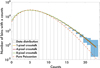 |
Fig. A.1 Counts distribution from a 128-s SiFAP2 lightcurve binned at 2.5 × 10⁻⁴ s (histogram), with binomial uncertainties (light blue area, 95% c.l.), compared with the expected distributions from pure Poisso-nian noise (orange dashed line), and GP noise arising from 1-, 4-, and 8-pixel crosstalk (solid lines). |
and from those derive the Pm(k) expected for that εct. We can then use Eq. (A.1) to construct the resulting expected total, crosstalk-affected distribution and compare it with the observed one at all k. By analysing a few tens of SiFAP2 observations from 2017 to 2023, we extracted values of εct which are on average ~7%, with small variations of ~1% at times where the instrumental setup was changed.
For all of them, we checked that the crosstalk-affected GP distribution we expected agreed well with the data. Figure A.1 shows one such example, for a 128-s-long segment of the observation of PSR J1023+0038 made on 2020/01/30: the histogram represents the distribution of pixel counts within 0.00025-s bins, with binomial 95% confidence levels for the underlying unknown distribution indicated by the light-blue shaded area (Clopper & Pearson 1934). The orange dashed line represents the distribution expected from pure Poissonian noise with average equal to the observed count average, while the solid lines indicate the expected distributions in the case of crosstalk-modified Poissonian noise, assuming 1-, 4-, and 8-pixel crosstalk: the agreement is very good for all three models, which, for our purposes, are virtually identical.
Moreover, we can also derive the expectation value and variance of the total distribution (e.g. Johnson et al. 2005; Gallego et al. 2013):
 (A.3a)
 (A.3a)
 (A.3a)
where  and E1 refer to the distribution of pixels excited by a single photon and only depend on εct (see Gallego et al. 2013); ϙ is the total dispersion index (in this case, equal to the overdispersion with respect to a Poissonian since for it E = σ2 = μ).
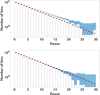 |
Fig. A.2 Upper panel - Power distribution of the PDS from the same data in Fig. A.1 (histogram), with binomial uncertainties (light blue area, 95% c.l.), compared with a χ2 distribution with two d.o.f. (burgundy points, normalized to the total number of powers). Lower panel - Same as upper panel, but after rescaling every power in the PDS by the dispersion index of the data. The χ2 distribution in the two panels is the same. |
Since our noise is well described by a GP distribution, we can adjust our analysis in one of two ways. The first method would be considering that as the expected photon distribution and revisiting all statistics and thresholds according to Eq. (A.3): the advantage of this method is that, when sure of the cause of the correlated noise, it can be used even outside PDS-based analysis (as in, e.g., Campa et al., in preparation). The second one is to exploit some of the properties of the noise distribution to still follow the usual approach, after a renormalization: if the noise tends to a white noise, the PDS can simply be renormalized by its dispersion index (see e.g. Israel & Stella 1996). This “tendency to white noise” of a distribution is formally proven if the sample mean of variables following that distribution tends to a Gaussian one. For generalized shot noise processes, including GP ones, a central limit theorem towards Gaussianity was demonstrated by Rice (1977). However, even if the noise were described by a different distribution, the range of distributions which tend to Gaussianity is quite extensive, including all finite-variance ones (the classical central limit theorem; see e.g. Feller 1971), all logconcave distributions (Klartag 2007), or equivalently strongly unimodal ones (Ibragimov 1956; Keilson & Gerber 1971), and more in general all the ones whose truncated second moment function varies slowly (e.g. Feller 1971, Chap. IX). The wider range of applicability of this second method makes it more robust to possible small differences of the real instrumental noise with respect to a given model.
Therefore, the following approach can be of use for PDS analysis whenever correlated noise is found in the data:
Check that the noise follows a distribution which tends to Gaussianity, in the sense described above;
If so, renormalize the PDS by dividing all powers by the dispersion index ϙ of the data, or, equivalently, half of the average high-frequency power;7
Carry out the PDS analysis on the renormalized spectra following the usual Leahy-normalized thresholds and probability assumptions, as in Sect. 4 and 5.
As an example of this, the upper panel of Fig. A.2 shows the distribution of powers (histogram) of the Leahy-normalized PDS of the same data from Fig. A.1, compared with a χ2 distribution with two degrees of freedom (normalized, burgundy points), which would be expected in the case of Poissonian noise (Leahy et al. 1983): the instrumental power distribution shows a significantly shallower slope than expected. If instead we first divide all power values by ϙ, we obtain the distribution in the lower panel: the agreement with the χ2 distribution, which is identical in the two panels, is now restored. In the present paper, we used this approach for all of the analysis described in the main text.
Appendix B Algorithm summary
In order to summarize the algorithm presented in Sect. 3 and help in the reproducibility of our results, we present here an outline of the whole semi-coherent search discussed in the main text.
SEMI-COHERENT SEARCH
for each frequency band considered do
COHERENT STEP
From the minimum of Porb and the maximum of a⊥ obtain the limits on each dimension in the coherent space through Eq. (4)
Find the largest order s* to contribute, for the chosen maximum mismatch μ*, to the Taylor expansion through Eq. (4)
Create a coherent template bank with all possible ν = (ν1,ν2,...,νs*) through Eq. (7)
for each segment m do
for each ν do
Compute τ(m)(ν) from the photons' detection times through Eq. (5)
Compute the PDS on the τ(m)(ν), obtaining Λ(m)
end for
end for
SEMI-COHERENT STEP
Create a semi-coherent template bank of combinations θ = (f, Porb, a⊥, Tasc)
for each segment m do
for each θ do
Compute ν(θ) through Eq. (4)
Find nearest neighbour in the coherent space
Sum the corresponding Λ(m) to Σ(θ)
end for
end for
if [Σ(θ)] > ΣPFA then
There is a detection (at the false alarm c.l. PFA; Eq. 10)
else
Find the Σ(θ) that maximizes the value of A through Eq. (13) to obtain the upper limit on the pulsed amplitude
end if
end for
Appendix C Significance thresholds for multiple dependent trials in χ2 random noise
Multi-trial searches inevitably entail facing the ‘multiple comparison problem’, i.e. the fact that given enough different trials computed, one can surely find significant structures in any statistic if the number of trials itself is not taken into account (see e.g. Tukey 1953; Hochberg & Tamhane 1987). Generally, procedures to do so put constraints on the familywise error rate (FWE), i.e. the chance of any false positives across all trials. In our case, we compare the summed power Σ obtained correcting the data for the binary motion at each template θ = (f, Porb, a⊥, Tasc) with the distribution of the power expected in the case of noise alone, a  distribution. Our null hypothesis (i.e. that only counting noise is present over the whole search region) is therefore rejected at a 1 - PFA confidence level if any Σ is above the threshold given by Eq. (10), which corrects for the number of trials n. The correction we used is the Dunn-Šidák one (Šidák 1967), which sets the level of false alarm probability on the single test as:
 (C.1)
(C.1)
This is commonly applied and for PFA values lower than ~5% it is essentially equivalent to the Bonferroni correction,  , which represents an upper limit on the FWE (see e.g. Hochberg & Tamhane 1987, Appendix 2).
The Bonferroni bound is very general, and makes no assumption about the independence of the trials computed. If however the values of the statistic considered are correlated, it tends to be conservative (e.g. Nichols & Hayasaka 2003; Worsley et al. 2004). Let us take as an example the summed powers Σ obtained in Sect. 7: the upper panel in Fig. C.1 shows the distribution of the Σ values for dataset D2 over the whole binary parameter space for the frequency interval 1349 - 1450 Hz, which is consistent with noise following a  distribution (here, M = 58). Nonetheless, since our template grid is dense to avoid potentially missing signals, the noise realizations at templates close to one another will not be completely independent: the photons’ detection time corrections for close combinations of binary parameters will be similar, and that in turn will affect the PDS. We follow the approach used in the Appendix of Nieder et al. (2019) to study the distribution of the maxima within subsets of our data: since in the analysis we kept the orbital period fixed, we have a 3D parameter space in f, a⊥, and Tasc which we divide in three dimensions in 404 × 139 × 15 pieces, respectively. We thus obtain 842 340 non-overlapping subsets of our parameter space, and for each of those we find the maximum value value of Σ. The distribution of these maxima is shown as the light blue histogram in Fig. C.1, lower panel, compared to the expected probability density of the n-trials-corrected
  distribution (dashed black line) which can be obtained by taking the derivative of Eq. (9) with respect to Σ:
 (C.2)
(C.2)
the number of trials in this case is n = 1920, i.e. the number of templates in each subset. As an additional comparison, the orange histogram represents the distribution of the Σ maxima calculated over the same number of non-overlapping subsets of our parameter space, this time however building the subsets from randomly shuffled points: clearly doing so removes the correlations in the single subsets, and the distribution follows again what is expected from purely independent trials. Therefore, in the correlated case most of the distribution of the maxima of our χ2 noise is skewed towards lower powers, but gradually approaches the behaviour of the uncorrelated case for the highest powers. This is perfectly consistent with what is expected from random field theory, in which the χ2 field for non-independent noise realizations was first studied by Worsley (1994). Later studies yielded ways to quantitatively assess the statistical significance of fluctuations for that field (Worsley et al. 1996; Worsley 2001): nevertheless, for high values of the χ2 statistic, the ones we are more interested in, the Bonferroni correction provides the tightest bound to the FWE and therefore to PFA (Nichols & Hayasaka 2003; Worsley et al. 2004; Taylor et al. 2007). This ensures that the sensitivity thresholds quoted across the rest of the paper are correct, at most being conservative. The same check was done at all frequency intervals for both Sco X-1 datasets, yielding the same results.
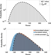 |
Fig. C.1 Upper panel - Power distribution of all of the Σ values obtained in the analysis of the 1349 - 1450 Hz interval for dataset D2 (see Sect. 7). The histogram was renormalized to the number of Σ values considered, i.e., the 51712 × 695 × 45 templates (over the f, a⊥, and Tasc dimensions). The dashed line is the expected |


All Tables
All Figures
|
Fig. 1 Maximum values of the summed power Σ, regardless of the corresponding orbital parameter combination, in the 50-1550 Hz frequency range, on a SiFAP2 observation of PSR J1023+0038. The dashed black line represents the 1% false-alarm threshold, which instead is calculated for all the combinations explored. |
| In the text | |
|
Fig. A.1 Counts distribution from a 128-s SiFAP2 lightcurve binned at 2.5 × 10⁻⁴ s (histogram), with binomial uncertainties (light blue area, 95% c.l.), compared with the expected distributions from pure Poisso-nian noise (orange dashed line), and GP noise arising from 1-, 4-, and 8-pixel crosstalk (solid lines). |
| In the text | |
|
Fig. A.2 Upper panel - Power distribution of the PDS from the same data in Fig. A.1 (histogram), with binomial uncertainties (light blue area, 95% c.l.), compared with a χ2 distribution with two d.o.f. (burgundy points, normalized to the total number of powers). Lower panel - Same as upper panel, but after rescaling every power in the PDS by the dispersion index of the data. The χ2 distribution in the two panels is the same. |
| In the text | |
|
Fig. C.1 Upper panel - Power distribution of all of the Σ values obtained in the analysis of the 1349 - 1450 Hz interval for dataset D2 (see Sect. 7). The histogram was renormalized to the number of Σ values considered, i.e., the 51712 × 695 × 45 templates (over the f, a⊥, and Tasc dimensions). The dashed line is the expected |
| In the text | |
Current usage metrics show cumulative count of Article Views (full-text article views including HTML views, PDF and ePub downloads, according to the available data) and Abstracts Views on Vision4Press platform.
Data correspond to usage on the plateform after 2015. The current usage metrics is available 48-96 hours after online publication and is updated daily on week days.
Initial download of the metrics may take a while.