| Issue |
A&A
Volume 707, March 2026
|
|
|---|---|---|
| Article Number | A165 | |
| Number of page(s) | 13 | |
| Section | Interstellar and circumstellar matter | |
| DOI | https://doi.org/10.1051/0004-6361/202556889 | |
| Published online | 12 March 2026 | |
Magnetic threads and gravity: ALMA observations of the infrared dark cloud G14.225-0.506
1
Institut de radioastronomie millimétrique (IRAM),
300 rue de la piscine,
38406
Saint Martin d’Hères,
France
2
Université Paris-Saclay, Université Paris Cité, CEA, CNRS,
AIM,
91191
Gif-sur-Yvette,
France
3
Institut de Ciències de l’Espai (ICE, CSIC),
Can Magrans s/n,
08193
Cerdanyola del Vallès,
Catalonia
4
Institut d’Estudis Espacials de Catalunya (IEEC),
Campus del Baix Llobregat–UPC, Esteve Terradas 1,
08860
Castelldefels, Catalonia,
Spain
5
Departament de Física Quàntica i Astrofísica (FQA), Universitat de Barcelona (UB),
Martí i Franquès 1,
08028
Barcelona, Catalonia,
Spain
6
Institut de Ciències del Cosmos (ICCUB), Universitat de Barcelona,
Martí i Franquès 1,
08028
Barcelona, Catalonia,
Spain
7
National Astronomical Observatory of Japan,
2-21-1 Osawa, Mitaka, Tokyo
181-8588,
Japan
8
Center for Astrophysics | Harvard & Smithsonian,
60 Garden Street, Cambridge, MA
02138,
USA
9
Academia Sinica, Institute of Astronomy and Astrophysics,
Taipei
10617,
Taiwan
10
Department of Physics, National Sun Yat-sen University,
No. 70, Lien-Hai Road, Kaohsiung City
80424,
Taiwan,
ROC
11
School of Astronomy and Space Science, Nanjing University,
Nanjing
210023,
PR China
12
Key Laboratory of Modern Astronomy and Astrophysics (Nanjing University),
Ministry of Education, Nanjing
210023,
PR China
13
Astronomy Department, University of Virginia, Charlottesville,
VA
22904,
USA
14
Institute of Astronomy & Department of Physics Institute of Astronomy and Department of Physics, National Tsing Hua University,
Hsinchu
300044,
Taiwan
★ Corresponding author: This email address is being protected from spambots. You need JavaScript enabled to view it.
Received:
18
August
2025
Accepted:
22
January
2026
Abstract
Context. In the star formation process, the interplay between gravity, turbulence, and magnetic fields is significant, with magnetic fields apparently serving a regulatory function by opposing gravitational collapse. Nonetheless, the extent to which magnetic fields are decisive relative to turbulence and gravity, as well as the specific environments and conditions involved, remains uncertain.
Aims. This study aims to ascertain the role of magnetic fields in the fragmentation of molecular clouds into clumps down to core scales.
Methods. We examined the magnetic field as observed with ALMA at core scales (approximately 10 000 AU/0.05 pc) toward the infrared dark cloud (IRDC) G14.225-0.506, focusing on three regions with shared physical conditions. We juxtaposed these data with prior observations at the hub-filament system scale (approximately 0.1 pc).
Results. Our findings indicate a similar magnetic field strength and fragmentation level between the two hubs. However, distinct magnetic field morphologies have been identified across the three regions where the polarized emission is detected. In region N (i.e., the northern Hub: Hub-N), the large-scale magnetic field, perpendicular to the filamentary structure, persists at smaller scales in the southern half; however, it becomes distorted near the more massive condensations in the northern half. Notably, these condensations exhibit signs of impending collapse, as evidenced by supercritical mass-to-flux values. In the region S (i.e., the southern Hub: Hub-S), the magnetic field is considerably inhomogeneous among the detected condensations and we did not observe a direct correlation between the field morphology and the condensation density. Lastly, in an isolated dust clump located within a southern filament of Hub-N, the magnetic field aligns parallel to the elongated emission, suggesting a transition in the field geometry.
Conclusions. The magnetic field shows a clear evolution with spatial scales. We propose that the most massive condensations detected in Hub-N are undergoing gravitational collapse, as revealed by the relative significance of the magnetic field and gravitational potential (ΣB) and mass-to-flux ratio. The distortion of the magnetic field could be a response to the flow of material as a result of such a collapse.
Key words: stars: formation / stars: massive / ISM: clouds / ISM: magnetic fields
© The Authors 2026
 Open Access article, published by EDP Sciences, under the terms of the Creative Commons Attribution License (https://creativecommons.org/licenses/by/4.0), which permits unrestricted use, distribution, and reproduction in any medium, provided the original work is properly cited.
This article is published in open access under the Subscribe to Open model. This email address is being protected from spambots. You need JavaScript enabled to view it. to support open access publication.
1 Introduction
The evolution of filamentary molecular clouds, the site of formation of massive stars, is a complex process involving gravitational force, turbulence, and magnetic fields. These processes play out across a vast range of spatial and density scales. Among the key physical agents involved, the magnetic field plays a significant role in the formation and fragmentation of filaments, as well as in the collapse of dense cores. Hence, it is an essential ingredient to develop a comprehensive model of star formation (Maury et al. 2022; Pattle et al. 2023).
Several models have been proposed to explain the collapse and fragmentation process of molecular clouds in the frame of high-mass star formation. For example, massive stars form in massive and turbulent cores, as detailed in the work by McKee & Tan (2003). In addition, turbulence is the property that triggers fragmentation in the frame of the inertial inflow model (Padoan et al. 2020). Star mergers have also been proposed as a possible explanation (Bonnell et al. 1998). Another possible scenario is global hierarchical collapse (GHC; Vázquez-Semadeni et al. 2019), where the cloud would collapse into filaments that would channel the material toward hubs, which are defined as sites where the filaments converge. In addition, Gómez et al. (2018) suggests an MHD model and explores the morphology of the magnetic field. The authors have predicted a filament evolution very similar to that of the GHC model, where the magnetic field presents a U-shaped due to the accretion toward and along the filament.
To measure the magnetic field in the interstellar medium, we must resort to the interaction of the magnetic field with its environment (Hildebrand et al. 2000). It is thought that interstellar grains are partially aligned with the magnetic field (Davis & Greenstein 1951), specifically with their major axis perpendicular to it, producing linearly polarized thermal emission perpendicular to the magnetic field direction. In addition, several techniques have been developed to estimate the magnetic field strength from polarized dust thermal emission, such as the Davis-Chandrasekhar-Fermi (DCF) method Davis & Greenstein (1951); Chandrasekhar & Fermi (1953) and intensity gradient (IG) techniques Koch et al. (2012a).
Over the past decade, numerous observational campaigns have been conducted, targeting both low- and high-mass sources (e.g., Zhang et al. 2014; Palau et al. 2021). In parallel, studies have focused on filamentary regions across a range of spatial scales (from several parsecs down to 0.01 pc) such as those toward NGC 6334 (Li et al. 2015; Cortés et al. 2021; Arzoumanian et al. 2021; Wu et al. 2024), G34.43+0.24 (Tang et al. 2019), and SDC18.624-0.070 (Lee et al. 2025).
Large surveys have also explored the role of magnetic fields in the fragmentation process, revealing a tentative correlation between fragmentation and the mass-to-flux ratio (Palau et al. 2021; Huang et al. 2025). This result further supports the idea that magnetic fields play a significant role in the fragmentation process.
Understanding the evolution of magnetic fields across spatial scales (from molecular clouds to dense cores) is essential for building a comprehensive picture of star formation. Various studies have aimed to trace this evolution (e.g., Wu et al. 2024). For example, Pillai et al. (2020) observed a change in magnetic field orientation: from perpendicular to the filament in low-density regions to parallel in high-density regions in a scheme resembling the one proposed by Gómez et al. (2018). A similar transition was reported by Kwon et al. (2022) in the Serpens Main molecular cloud. At even smaller scales, Koch et al. (2022) resolved a network of dust lanes and streamers connecting dense cores, finding that the magnetic field is generally aligned with these structures.
In this context, we focus on the IRDC G14.225–0.506 (hereafter IRDC G14.2), located southwest of the H II region M17. While its distance was initially estimated at 1.98 kpc (Xu et al. 2011), more recent Gaia DR2 data suggest a range of 1.49–1.57 kpc (Zucker et al. 2020). For the present work, we adopted a distance of 1.6 kpc as in Díaz-Márquez et al. (2024). The IRDC G14.2 exhibits a prominent network of filamentary structures with two main hubs, named Hub-N and Hub-S. (Busquet et al. 2013; Chen et al. 2019). Both are associated with a rich population of protostars and young stellar objects (YSOs; Povich & Whitney 2010; Povich et al. 2016; Ohashi et al. 2016; Busquet et al. 2016; Díaz-Márquez et al. 2024; Zhao et al. 2025). In addition, Chen et al. (2019) identified a third hub candidate, referred to as Hub-C, located at the intersection of two filamentary structures. These hubs are warmer, denser, and more massive than the surrounding filaments, and they exhibit larger velocity dispersions (Busquet et al. 2013).
Previous polarimetric observations toward the region include the work of Santos et al. (2016). They carry out optical and near-infrared (NIR) polarimetric observations to map the magnetic field surrounding the filamentary structures. They find the magnetic field morphology in the POS to be perpendicular to both the large-scale molecular cloud and the filaments, deriving the magnetic field strength, Alfvén Mach numbers, and mass-to-flux ratio that point out toward a sub-Alfvénic and super-critical regime, suggesting that magnetic fields cannot prevent gravitational collapse.
Busquet et al. (2016) presents 1.3 mm continuum emission observation toward G14.2 carried out with the Submillimeter Array with angular resolution in the range (1′′−3′′) as well as 870 μm (APEX) at 18′′.6 and 350 μm (Caltech Submillimeter Observatory, CSO) ones at 9′′.6 resolution. They found that while the northern Hub (Hub-N), understood as regions of greater density where the filaments intersect, presents four fragments, while the southern Hub (Hub-S) is more fragmented, showing up to 13 fragments. Interestingly, these authors found that all derived physical properties (e.g., density and temperature profiles, the level of turbulence, magnetic field around the hubs, and the rotational-to-gravitational energy) are remarkably similar in both hubs.
The magnetic field strength was estimated from CSO polarimetric observation (350 μm) at hub and filament scales (∼ 0.1 pc, ∼ 10′′ angular resolution). Using three different methods, the authors obtained a magnetic field strength of 0.6−0.8 mG in Hub-N and 0.1−0.2 mG in Hub-S, which is consistent with the lower fragmentation level observed in the Hub-N by Busquet et al. (2016). In addition, the B-field-to-gravity force ratio was estimated toward Hub-N, finding a gravitational collapse domain (Añez-López et al. 2020).
In this paper, we present new ALMA polarimetric observations at 1.39 mm with ∼ 2′′ resolution (∼ 3200 AU) toward the two hubs and three additional fields along the filament structure of G14.225-0.506 to investigate the magnetic field down to core scales. This cloud is part of 17 massive protostellar cluster forming clumps observed in full polarization mode with the ALMA main array under project 2017.1.00793.S (PI: Qizhou Zhang). The overview of the survey can be found in Zhang et al. (2025) and detailed analyses of the infrared dark cloud (IRDC) G28.34+0.06 and NGC 6334 can be found in Liu et al. (2020, 2023a, b, 2024), respectively. The paper is structured as follows. Section 2 describes the observation set up and we present the results of the continuum emission in Sect. 3. In Sect. 4, we present the magnetic field morphology and strength, and its analysis through the magnetic field significance (ΣB maps) is presented in Sect. 5. Finally, Sect. 6 provides a discussion and Sect. 7 the conclusions of this work.
2 Observations
The data presented here toward G14.2 is part of the ALMA project 2017.1.00793.S. The observations were done in full polarization mode at 1.39 mm (band 6) with the C43-4 and C43-1 configurations. The observations were performed between March and September 2018 for the C43-4 configuration and in July 2018 for the C43-1 configuration. We observed three and four contiguous single fields in Hub-N and Hub-S, respectively. We also observed three pointings in the filaments associated with the Hub-N, named F1, F2, and F3. Notably, the F1 field coincides with the Hub-C candidate identified by Chen et al. (2019). The observed primary beams are shown in Fig. 1. The correlator was configured to observe three wideband spectral windows of 1875 MHz each, centered at 216.4, 218.5, and 233.5 GHz. In addition, four narrowband spectral windows of 58.6 MHz and a spectral resolution of 0.32 km s−1 were used to observe the CO(3−2), N2 D+(3−2),13 CS(5−4), and OCS (19–18) spectral lines. The Stokes I continuum emission along with line data from C43-1 are presented in Zhao et al. (2025). In this paper, we present the linear polarization of the continuum emission.
The imaging process was made using the CASA software, specifically with the 6.5.5 version. The maps presented here were done using natural weighting with a Gaussian taper to the visibilities with a width of 50 kλ. In addition, we only used visibilities corresponding to baselines shorter than 500 kλ. This maximizes the polarization signal at scales of a few thousand AU (2−10′′). The resulting synthesized beam is 2′′ 37 × 22′′ 10 with a position angle of −78.6°. The root-mean-square (rms) noise of the maps (σqu) was 0.048 mJy beam−1 for the Stokes Q and U. For Stokes I (σI) was higher, 0.12 mJy beam−1, probably due to the limited dynamic range. The signal-to-noise ratio (S/N) achieved is around 1800. The final images were corrected for the primary beam response using the CASA task impbcor to the 20% sensitivity level of the Stokes I primary beam model. To calculate the polarization intensity, we applied Ricean debiasing and we also applied a threshold of ten times the rms in Stokes I. The polarization images were computed using a cutoff of three times the Q and U rms. Position angles were computed as θ=1/2 arctan 2(U/Q). Only magnetic field segments within 40% of the primary beam were considered toward mosaics, which represents a relaxation of the suggested limit for a single point by ALMA (33.33%), which we have applied in the individual point, which is justified by the overlap of pointing that occurs in the mosaics (Hull et al. 2020). We obtained magnetic field morphology in the POS, assuming radiative alignment torques (RAT) and it was traced by linearly polarized emission and rotating polarization segments by 90° (see review by Lazarian et al. 2015).
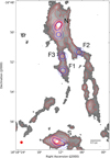 |
Fig. 1 CSO continuum emission at 350 μm (gray map) and red contours, which depict [3, 6, 9, 15, 25, 35, 45, 55, 65, 75, 85, and 95] times the rms noise (80 mJy beam−1). The red and black circles in the lower left corner show the CSO and ALMA beam size, respectively. Blue contours represent the 80%, 40%, and 33% levels of the ALMA primary beam for each target region, labeled N, F1, F2, F3, and S. |
3 Dust continuum emission
Figures 2 and 3 show the 1.39 mm dust continuum emission toward the three observed regions where polarized emission is detected (N, S, and F1). The continuum emission, where the extremely high S/N (1800) allows for the denser cores as well as the weaker filamentary emission connecting them to be traced; this is consistent with previous observations at similar scales (Busquet et al. 2016; Zhao et al. 2025).
The continuum emission toward region N shows a main elongated distribution with a north-south orientation, along the dense gas filament seen in NH3 and N2 H+(Busquet et al. 2013; Chen et al. 2019), and eight emission peaks along it (see Fig. 2, top panels). Toward region S, the observations resolve multiple emission enhancements distributed along a generally elongated and curved structure extending from the north to the southeast (see Fig. 2, bottom). The locations and previous detections within each region are detailed in Table A.1.
The continuum emission toward region F1 also exhibits an elongated morphology oriented from northeast to southwest (see Fig. 3), consistent with the main axis of the filament traced by CSO observations (see Fig. 1). This region is considered a candidate hub and displays both warm and compact ammonia emission (Busquet et al. 2013; Chen et al. 2019). The continuum emission toward region F2 reveals a rotated L-shaped structure, consisting of two elongated features that converge at an angle of approximately 90° (see Fig. B.1). Three intensity enhancements are observed: one on each arm of the structure and a third at their intersection. The continuum emission in region F3 also presents a filamentary morphology, oriented north to south, and contains a single prominent emission peak.
To avoid biases in the area selection, we performed the analysis by dendrogram (Rosolowsky et al. 2008) to extract the hierarchical structure in the present ALMA observation after rebinning the maps by a factor of 3 to achieve a pixel/beam = 1/3, where we have: beam =2′′.37 × 2′′.10 and pix =0′′.8 × 0′′.7. Thus, we were able to study the B field in selected regions with enough independent polarization measurements. We adopted a minimum significance threshold of 1σI(σI=0.12 mJy. beam−1) for each leaf, along with a requirement that each leaf span an area equivalent to at least three beams to be considered independent. These criteria represent a relaxation of those used in the dendrogram analysis by Zhao et al. (2025), allowing us to achieve a better alignment with the objectives outlined above. For the purposes of this analysis, we considered structures with no substructure (i.e., leaves in the dendrogram vocabulary) within each field (see Fig. 2, left and Fig. 3 for the regions N and S, and F1, respectively). Henceforth, we refer to these leaves as condensations.
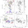 |
Fig. 2 Continuum emission at 1.39 mm toward region N (upper panel) and region S (bottom panel). Contours depict [10, 20, 30, 40, 50, 60, 70, 80, 90, 100, 150, 300, 500, and 700] times the rms noise (0.12 mJy beam−1), overlapped with magnetic field segments in blue, where thin and thick segments depict segments within the inner 50% and 40% of the primary beam model, respectively. Red segments show the CSO magnetic field at 350 μm, where thin and thick segments indicate a polarization intensity between two and three sigmas and higher than three times sigma, respectively (CSO sigma =0.02 Jybeam−1 Añez-López et al. 2020). Color contours show the leaves from the dendrogram analysis, while the black labels present the corresponding ID label. The blue solid circle in the bottom left corner of each panel depict the ALMA beam size. The pink triangle shows the H2 O maser detected in Wang et al. (2006). Green tripods show cores detected with the SMA telescope at 1.3 mm (Busquet et al. 2016). Yellow and purple tripods depict radio sources detected at 6 cm (C-band) and at 3.6 cm (X-band) by Díaz-Márquez et al. (2024), respectively. White tripods show NH3 cores detected by Ohashi et al. (2016). |
4 Magnetic field
In this section, we present the magnetic field morphology toward each region where the polarized emission is detected at core scales (<10 000 AU/0.05 pc); namely, in the N, S, and F1 regions. In Figs. 2 (top-left) and 2 (bottom-left), and 3, we show the morphology of the plane-of-sky (POS) magnetic field in region N and in S, and F1, respectively, where only segments with a signal greater than 3σqu are displayed. These figures also include magnetic field observations at 350 μm from the CSO at scales of ∼ 0.1 pc, which were previously presented in Añez-López et al. (2020). In Figs. 4 (top), 4 (bottom), and 5, we show the histogram of the position angle distribution for the regions N, S, and F1, respectively, where the median value is indicated by a black line.
We also show the polarization overall orientation in the H and R bands detected by Santos et al. (2016).
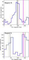 |
Fig. 4 Magnetic field position angle histogram toward region N (top) and S (bottom). Black solid lines depict the angle median value i.e., 95° for region N and (44°, 153°) for region S. Red dotted lines show the main direction of the CSO magnetic field orientation, 105° and (33°, 134°) for regions N and S, respectively, as shown in Añez-López et al. (2020). Magenta dashed line is set perpendicular to the main filament orientation (i.e., F10-E, 100°, Busquet et al. 2013). Magenta solid and dotted lines indicate the overall orientation of the polarization in the H and R bands, respectively (Santos et al. 2016). |
4.1 Hub-N
The magnetic field segments in region N are primarily oriented perpendicular to the elongated continuum emission (Fig. 2, top-left), where the median value is 95° (Fig. 4, top). The median position angle closely matches the value reported by CSO(105°) and is perpendicular to the main filament orientation (10°) reported by Busquet et al. (2013).
However, the main magnetic field orientation is altered in the vicinity of the main peak emission, coinciding with the locations of the condensations N-5, N-7, and also N-8. This behavior is reflected in the bimodal distribution shown in the histogram (Fig. 4, top), with a secondary peak around 0°/180°. Therefore, even though we see that at larger scales (CSO, angular resolution ∼ 10′′) the magnetic field appears to be homogeneous and perpendicular to the filament orientation, at a higher angular resolution (∼ 2′′), the ALMA observations show distortions in the environments of the most massive condensations (see Table 1).
To illustrate the distortion of the magnetic field, we present in Fig. 6 (top-left) the relative position angle with respect to the larger scale, computed within every condensation in the regions. The angular resolution inequality prevents us from comparing pixel by pixel, while we can compute the difference between the ALMA position angle for each pixel and the corresponding averaged CSO value for each condensation. Figures 6 (top-left) and also 6 (top-right) that present the relative angle histogram, showing that the CSO magnetic field prevails at ALMA scales throughout the elongated continuous emission, basically in N-2 and N-4 condensations. However, it is clearly distorted when we approach N-8 and especially in the N-7 environment.
Figure D.1 (left) presents the polarization fraction map toward region N, whose averaged value is 3.68%. We found the lowest polarization values (<2%) toward the main emission peaks, N-7 (orange) and N-8 (yellow). These results are summarized in Table 1.
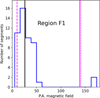 |
Fig. 5 Magnetic field position angle histogram, toward region F1. Black solid line depicts the median value over the distribution (∼ 26°). Magenta dashed lined shows the orientation of main filament orientation (∼ 10°) Busquet et al. (2013). Magenta solid and dotted lines indicate the overall orientation of the polarization in the H and R bands, respectively (Santos et al. 2016). |
4.2 Hub-S
Figure 2 (bottom-left) presents the POS magnetic field morphology toward the region S. Region S displays a less regular angle distribution than region N (see Fig. 4, bottom). It also shows a bimodal distribution, with two main peaks at 44° and 153° that are in agreement with the distribution previously detected at filament scales with the CSO telescope (33° and 134° Añez-López et al. 2020). Table 1 summarizes average angles and standard deviation for each condensation.
We also present the relative angle map of the magnetic field relative to the field previously detected by the CSO in Fig. 6-bottom-left. Unfortunately, previous CSO detections toward this region are very scarce, so it is only possible to calculate the relative angle in two condensations, S-3 (magenta) and S-6 (green). High values of around 90° are present at the peak emission in both S-3 and S-6 condensations as shown in Fig. 6 (bottom-right). Toward S-6, the vast majority of the vectors are distorted by more than 60°, whereas S-3 exhibits a more spread distribution, with a peak around 30°.
Figure D.1 (right) shows the polarization percent map toward the region S, with an average value of ∼ 5%. Table 1 summarizes the results of the mean values of the polarization percentage on each condensation, along with their dispersion. The lower values are found in S-3 and S-2 (1.29 and 1.41%, respectively), while the larger values (5.39% and 5.33%) are found toward S-1 and S-5.
Results of the condensation analysis.
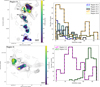 |
Fig. 6 Relative position angle map and histogram (left and right, respectively) of the magnetic field observed by current ALMA ∼ 2′′ ar and by former CSO ∼ 10′′ ar toward region N (upper) and S (bottom). |
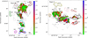 |
Fig. 7 ΣB map in color toward region N. Black and colored contours show the Stokes I and the leaves found via the dendrogram analysis. |
4.3 Region F1
Figure 3 presents the POS magnetic field morphology toward region F1, which has been identified as a hub candidate (Chen et al. 2019). The magnetic field exhibits a predominant northeast to southwest orientation, aligned with the continuum emission. However, we note that the magnetic field in the vicinity of the peak emission (∼ 18 h 18 m 11.30,−16° 52′ 33′′) deviates to a north-south-like orientation. Figure 5 presents the histogram of the position angles toward region F1, where the predominant orientation is about 26°, which is in good agreement with the main orientation of the filament (10°; Busquet et al. 2013). Unfortunately, the CSO polarization observations used for comparison in previous sections do not cover this specific field of view, preventing a direct comparison. Table 1 summarizes the main results of the magnetic field position angle analysis within the condensation where the magnetic field is detected.
In Fig. D.1 (bottom), we show the polarization percent map toward the region F1. Values range between 0.6 and 4.9%, with an averaged value of 2.1%. We found the lowest polarization (<2%) percent toward the peak emission. Table 1 presents the averaged polarization percent, 2.87%, and its standard deviation, 1.50%.
5 Magnetic field versus gravitational potential: the IG-method
We computed the relative significance of the magnetic field and gravitational potential in order to develop an analysis analogous to that originally proposed by Koch et al. (2012a), later refined and tested by Koch et al. (2013, 2014). This method (henceforth referred to as the IG method) assumes that emission intensity is due to the transport of matter, which is driven by a combination of magnetohydrodynamic forces (MHD). Therefore, the intensity gradient would measure the motion direction. Then, solving the MHD equations for the magnetic field, the authors provide an expression for the magnetic field in the POS as a function of measurable variables on a 2D map, expressed as
![Mathematical equation: $\left[\frac{B_{\mathrm{pos}}}{G}\right]=\sqrt{\frac{sin \psi}{sin \alpha}(\nabla P+\rho \nabla \phi) 4 \pi R},$](/articles/aa/full_html/2026/03/aa56889-25/aa56889-25-eq1.png) (1)
where the density (ρ) is in g cm−3, the gravitational potential gradient (∇φ) is in cm s−2, and the B-field curvature radius (R) is in cm. The resulting B-field is in Gauss. For simplicity, we neglected the pressure gradient (∇P), which is typically small compared to gravity potential. Here, ΣB is the magnetic field significance, according to the following equation,
(1)
where the density (ρ) is in g cm−3, the gravitational potential gradient (∇φ) is in cm s−2, and the B-field curvature radius (R) is in cm. The resulting B-field is in Gauss. For simplicity, we neglected the pressure gradient (∇P), which is typically small compared to gravity potential. Here, ΣB is the magnetic field significance, according to the following equation,
 (2)
where Ψ and α are the angles in the POS between the orientation of local gravity and intensity gradient, as well as those between polarization and intensity gradient, respectively. Values of ΣB greater than or less than unity indicate whether the magnetic field force is able to prevent gravitational collapse or not, respectively. Local gravity is computed through the surrounding mass distribution in any position on the map, where the main assumption is to use the dust emission as a proxy for the gas mass.
(2)
where Ψ and α are the angles in the POS between the orientation of local gravity and intensity gradient, as well as those between polarization and intensity gradient, respectively. Values of ΣB greater than or less than unity indicate whether the magnetic field force is able to prevent gravitational collapse or not, respectively. Local gravity is computed through the surrounding mass distribution in any position on the map, where the main assumption is to use the dust emission as a proxy for the gas mass.
This technique, which is part of a set of methods for inferring the role of the magnetic field in the collapse based on the geometry of the magnetic field, as well as on the density structures, has been tested extensively and applied in various studies (e.g., Tang et al. 2009; Koch et al. 2014, 2018, 2022). Following this recipe, we calculated the ΣB maps toward regions N, S, and F1, as well as the average magnetic field strength for each condensation. Figure 7 (left) presents the ΣB map of region N, revealing that most values are below 1. This suggests that gravitational collapse is the dominant force over magnetic tension in the region. Figure 7 (right) shows the ΣB-map toward the region S, which appears to be dominated by values lower than 1. The lower ΣB averaged values, typically under 0.5, are found toward S3, S6, and S8 condensations. Overall, every condensation shows gravitational collapse dominance. Table 1 summarizes ΣB averaged values, standard deviation, and percentage of pixels that exhibit values under 1 for every condensation.
Figure 8 presents the ΣB-map toward region F1 (F1-2), revealing a predominance of values below unity, which indicates gravitational dominance over magnetic support. Table 2 includes the calculation of the magnetic field strength using the method presented above, as well as the one calculated using the DCF-C method (Davis 1951; Chandrasekhar & Fermi 1953) by means of Eq. (2) of Crutcher et al. (2004):
 (3)
where ρ is the gas density (g/cm3), σv is the velocity dispersion (km/s), σPA is the polarization angle dispersion, n(H2) is the gas number density
(3)
where ρ is the gas density (g/cm3), σv is the velocity dispersion (km/s), σPA is the polarization angle dispersion, n(H2) is the gas number density  is the linewidth (km/s), and Q is a factor of order unity. We also computed the version presented by Falceta-Gonçalves et al. (2008) (DCF-FC), which allows us to avoid the limitation regarding the angle dispersion,
 (4)
(4)
In addition, we applied the correction presented in Heitsch et al. (2001) (DCF-H), that reflects equipartition between kinetic and magnetic energy,
 (5)
(5)
In all three cases, we considered a Q factor of 0.28, which is well suited for the small scales and high densities considered here (Liu et al. 2021, 2022). We estimated the column density and mass for every condensation from the current flux observation and the kinematic temperature of ammonia estimated in Busquet et al. (2013) by applying the optically thin approximation (Hildebrand 1983; Andre et al. 1993):
 (6)
where we assumed a dust opacity, κv, of 0.9 cm2 g−1 Ossenkopf & Henning (1994) and also a gas-to-dust ratio of 100 to compute the total mass.
(6)
where we assumed a dust opacity, κv, of 0.9 cm2 g−1 Ossenkopf & Henning (1994) and also a gas-to-dust ratio of 100 to compute the total mass.
Finally, following Hildebrand et al. (2009) and Houde et al. (2009, 2011), in Appendix E we show the fitted square root of the structure function (SF2) of the polarization orientation angles toward each region as a function of the separation between segments, expressed as
 (7)
where b (the intercept with the y-axis) shows the turbulent contribution to the angular dispersion, m2 is a constant, and σ2(l) is the uncertainty on the polarization angles. We consider a separation no smaller than one third of the beam (i.e., one pixel). Then, we can estimate the magnetic field strength as follows (DCF-SF):
(7)
where b (the intercept with the y-axis) shows the turbulent contribution to the angular dispersion, m2 is a constant, and σ2(l) is the uncertainty on the polarization angles. We consider a separation no smaller than one third of the beam (i.e., one pixel). Then, we can estimate the magnetic field strength as follows (DCF-SF):
 (8)
(8)
We omitted the DCF-C method (Eq. (3)) results in cases where the standard deviation of polarization angles exceeds 25°, as this violates the small-angle approximation underlying the tangent-angle equivalence. While the four DCF methods give similar results ranging from 0.2 to 2.3 mG, the method developed by Koch et al. (2012a) reflects a wider range from 0.8 to 15.9 mG (see Table 2). Later in this work, we discuss the validity of these methods at the scales considered here. This method is expressed as
 (9)
(9)
The mass-to-flux ratios (λ) computed using Eq. (9), presented in Crutcher et al. (2004), are shown in Table 2. The mass-to-flux ratio can also be calculated independently of the magnetic field strength, as a function of the radius and the significance of the magnetic field (ΣB; see Koch et al. 2012b for details; see also Table 2).
Toward the most massive condensations, e.g., N-7, the mass-to-flux ratio exceeds unity, indicating a supercritical state, regardless of the method we used to estimate the magnetic field. However, in other cases (e.g., N-2, N-4, S-6), we have observed discrepancies depending on the method used, which we will discuss below (see Table 2).
Results of the condensation analysis.
6 Discussion
6.1 Mass-to-flux ratios
Quantifying the amount of mass per unit magnetic flux, known as the mass-to-flux ratio, is essential for understanding the influence of magnetic fields on star formation. In this study, we computed the mass-to-flux ratio using the IG method; namely, independently of the strength of the magnetic field and also from the magnetic field strength obtained using several DCF method variants (see Eq. (9)). For the more massive condensation studied during this work (N-7), both IG, DCF-FG, DCF-SF, and DCF-H methods agree on a supercritical state. However, for some other condensations (N-2, N-4, S-6), we find discrepancies among these methods.
To understand these discrepancies, we first looked at the magnetic field strength. In all cases, the IG method provides larger magnetic fields, with the difference ranging from a factor of two to one order of magnitude. Liu et al. (2021) suggested that the DCF method tends to overestimate the field. If the DCF method does indeed overestimate the magnetic field strength, leading to a lower mass-to-flux ratio, this could explain the mass-to-flux discrepancy across methods. However, this would also imply an even larger divergence in the field strength estimates between IG and DCF family methods.
Second, we must also consider uncertainties in the mass estimates. Our calculations exclude mass from the innermost tens of astronomical units, due to optical thickness, as well as the mass that was already accreted onto the protostar. Both omissions could contribute to an underestimation of the total mass (and, thus, the mass-to-flux ratio), which would reduce the discrepancies mentioned above.
Third, we must consider additional sources of uncertainty. For example, the estimation of the velocity dispersion has been identified as one of the greatest sources of uncertainty in the DCF analysis (Chen et al. 2022). In addition, geometrical effects, due to an inclined system, could also impact the DCF results (Gonçalves et al. 2005). On the other hand, the IG method is affected by the local turbulence field that could act as a contaminant. In addition, significant changes in temperature over a map would lead to a wrong estimation of the mass that would further lead to wrong gravity direction and therefore to wrong magnetic field strength, causing the method to fail (Koch et al. 2012a).
Finally, despite numerous sources of uncertainty that impact all existing methods for estimating the magnetic field (and, thus, the mass-to-flux ratio) almost all methods agree in pointing toward gravitational collapse in the most massive condensations (N-7 and S-3), where we also observe a greater distortion of the magnetic field compared to the field at larger scales. Furthermore, ΣB analysis indicates that the magnetic tension force is not able to hold the gravitational pull toward the condensation that dominates gravitationally in the region. All together supports the hypothesis that collapse has already begun and the consequent flow of matter toward sinks begins to have an impact on the morphology of the field that is drawn in Gómez et al. (2018); Suin et al. (2025).
6.2 Multiscale collapse
• Hub-N: Santos et al. (2016) presented the magnetic field morphology in the IRDC G14, around the cloud, in the optical and also at filamentary cloud scales in NIR. Añez-López et al. (2020) analyzed the magnetic field at filament scales (CSO). On these scales, where N-2, N-4, N-5, N-7, and N-8 are both embedded in the ∼ 0.3 pc Hub-N region, these authors observed that the orientation of the magnetic field becomes mostly perpendicular to the filament system, although it shows slight alterations in the peak emission environment. Over the course of the current work, we zoomed in on Hub-N, where the magnetic field on scales of ∼ 0.05 pc exhibits a largely uniform orientation in the southern half. In contrast, the northern half, where the bulk of the mass is concentrated, shows clear signs of magnetic field distortion. Overall, we can clearly see the transition of the magnetic field from the scales around the cloud (∼ 141°) up to filamentary cloud scales (∼ 139°) and filament scales (∼ 105°), ultimately reaching hub scales in the current observations (∼ 95°). We even see subregions with dramatic transitions of almost 90° (N7).
A similar behavior was reported by Koch et al. (2022), who presented envelope-to-core scale polarization observations of the high-mass star-forming region W51. They found a predominantly uniform field at large scales, with the first distortions appearing near the intensity peak and higher-resolution data revealing an additional substructure.
This overall magnetic morphology is consistent with theoretical models in which accreting material travels along magnetic field lines that lie perpendicular to the filament (Gómez et al. 2018). These models also predict an eventual flip in the field orientation as material flowing along the filament drags the field. For example, the N-7 region displays a bimodal distribution that was not present at larger scales: segments in the northern portion align with the large-scale magnetic field, whereas those in the southern portion are oriented perpendicular to it. This configuration would be compatible with accretion from the south, moving parallel to the filament’s major axis, that would shape the field.
• Hub-S: the scarce large-scale magnetic field detection prevents a complete comparison. The field substructure appears more complex and, in principle, its orientation does not correspond to the direction either perpendicular or parallel to the filaments. On the other hand, if we analyze the magnetic field in the Hub-S as a whole, we see an evident bimodal distribution that resembles that was previously observed at filament scales with the CSO telescope (see Fig. 4). However, individually, the condensations show magnetic field morphologies that, although uniform, deviate from the orientation at larger scales. One possible explanation is that we are resolving the common envelope of the condensations and, therefore, the region could be dominated by the collapse of multiple cores that drag the field within their area of influence. The influence of protostar feedback in the region may also be impacting the field morphology (Hull et al. 2020).
• F1: region F1 shows a magnetic field aligned with the elongated continuum emission, which roughly follows the orientation of the large-scale filament, as expected in a scenario where filaments transport material to the hubs (Gómez et al. 2018). This was described, for example, by Peretto et al. (2014) toward the IR dark filament SDC13.
In conclusion, we note that both hubs show a bimodal distribution of polarization angles and, in the case of Hub-N, it was not present at larger scales, with peaks separated by approximately 90°. In region S, this pattern has been previously observed with CSO data at ∼ 10′′ angular resolution. In region-N, the emergence of a second peak aligns with regions where the magnetic field becomes distorted, providing further evidence that gravity is starting to influence and bend the field away from its initial, large-scale orientation. In short, on filament scales, we see a magnetic field morphology that is compatible with accretion toward the filament itself; however, when we descend the analysis points to collapse toward the individual cores, which is in agreement with the GHC scheme (Gómez et al. 2018; Vázquez-Semadeni et al. 2019).
Finally, we observed a positive correlation between the median magnetic field distortion and the averaged density of the individual condensation in the range 2−9 × 10⁻⁶ cm−3; from this density onward, the correlation reverses (see Fig. 9). In the hub-filament system, observations show a similar alignment transition when the density increases (e.g., Pillai et al. 2020; Arzoumanian et al. 2021) as a consequence of material flows (Gómez et al. 2018; Suin et al. 2025). In addition, it is also plausible that the outflows present in the region (Zhao et al. 2025) have an impact on both the magnetic field morphology and also the filamentary structures (Suin et al. 2025). Thus, we cannot rule out a combination of factors affecting the morphology of the field.
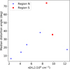 |
Fig. 9 Median distortion of the magnetic field as a function of the averaged number density computed for each individual condensation in both Hub-N and Hub-S, shown by the blue stars and red squares, respectively. |
7 Conclusion
In the present work, we analyzed ALMA polarization observations at 1.39 mm with 2′′ (3200 AU) angular resolution toward the IRDC G14.225-0.502, a region composed of two hub-like structures connected by a filament. Previous studies have suggested that these are twin hubs with differing magnetic field strength and fragmentation properties. By investigating the morphology and strength of the magnetic field at small scales, we reached several key conclusions.
First, polarized emission was detected in three out of the five observed fields. Specifically in Regions N, S, and F1 associated with Hub-N, Hub-S, and the Hub-C candidate, multiple emission enhancements were resolved across all five fields. On average, the magnetic field strength is a factor of two larger in the Hub-S. However, at the present resolution, Hubs N and S do not exhibit significant differences in their fragmentation levels according to the number of leaves reported by the dendrogram analysis.
Second, in region N, the magnetic field morphology is consistent with current models (GHC), where lateral material accretion shapes the magnetic field perpendicularly to the filament. In addition, the magnetic field distortion found toward the more massive condensations could be explained by the flow of material toward the main gravitational sinks within the Hub-N. However, star formation feedback cannot be ruled out as an ingredient, especially in the Hub-S, where we see a generally less homogeneous magnetic field.
Finally, the derived ΣB values, together with the mass-to-flux ratios, strongly support the interpretation that gravity is the prevailing force in these distorted regions. The areas associated with the second polarization angle peak not only show ΣB<1, indicating a supercritical state, but they also coincide with zones of maximum magnetic field distortion. Crucially, we were able to trace a clear transition in the magnetic field morphology from a uniform configuration to a more complex, gravity-influenced structure. This direct link between field morphology and the ΣB parameter provides compelling observational evidence that the effects of gravity are increasingly dominant with respect to magnetic support at smaller spatial scales, shaping the magnetic field during the early stages of core collapse.
Acknowledgements
We would like to thank the anonymous referee for their contribution to the improvement of the manuscript through their constructive comments. We acknowledge Dr. F. Alves for the constructive discussion and for sharing his perspective on the article. N.A.L. acknowledge financial support from the European Research Council (ERC) via the ERC Synergy Grant ECOGAL (grant 855130). G.B. and J.M.G. acknowledges support from the PID2020-117710GB-I00 grant funded by MCIN AEI/10.13039/501100011033 and from the PID2023-146675NB-I00 (MCI-AEI-FEDER, UE) program. J.M.G. and A.M. have been supported by the program Unidad de Excelencia María de Maeztu, awarded to the Institut de Ciències de l’Espai (CEX2020-001058-M). A.M. acknowledges support from the European Research Council (ERC) under the European Union’s Horizon 2020 research and innovation program (Grant agreement No. 101098309 – PEBBLES). J.L. is partially supported by Grant-in-Aid for Scientific Research (KAKENHI Number 23H01221 and 25K17445) of the Japan Society for the Promotion of Science (JSPS). H.B.L. is supported by the National Science and Technology Council (NSTC) of Taiwan (Grant Nos. 111-2112-M-110-022-MY3, 113-2112-M-110-022-MY3). Z.Y.L. is supported in part by NASA 80NSSC20K0533, NSF AST-2307199, and the Virginia Institute of Theoretical Astronomy (VITA). H.V.C. acknowledges financial support from National Science and Technology Council (NSTC) of Taiwan grants NSTC 112-2112-M-007-041. S.P.L. acknowledges support from the National Science and Technology Council (NSTC) of Taiwan under grants 109-2112-M-007-010-MY3, 112-2112-M-007-011, and 113-2112-M-007-004. This research made use of astrodendro, a Python package to compute dendrograms of Astronomical data (http://www.dendrograms.org/) and Astropy (http://www.astropy.org), also CASA version 6.5.5.
References
- Añez-López, N., Busquet, G., Koch, P. M., et al. 2020, A&A, 644, A52 [NASA ADS] [CrossRef] [EDP Sciences] [Google Scholar]
- Andre, P., Ward-Thompson, D., & Barsony, M., 1993, ApJ, 406, 122 [NASA ADS] [CrossRef] [Google Scholar]
- Arzoumanian, D., Furuya, R. S., Hasegawa, T., et al. 2021, A&A, 647, A78 [NASA ADS] [CrossRef] [EDP Sciences] [Google Scholar]
- Bonnell, I. A., Bate, M. R., & Zinnecker, H., 1998, MNRAS, 298, 93 [Google Scholar]
- Busquet, G., Zhang, Q., Palau, A., et al. 2013, ApJ, 764, L26 [NASA ADS] [CrossRef] [Google Scholar]
- Busquet, G., Estalella, R., Palau, A., et al. 2016, ApJ, 819, 139 [Google Scholar]
- Chandrasekhar, S., & Fermi, E., 1953, ApJ, 118, 113 [Google Scholar]
- Chen, H.-R. V., Zhang, Q., Wright, M. C. H., et al. 2019, ApJ, 875, 24 [Google Scholar]
- Chen, C.-Y., Li, Z.-Y., Mazzei, R. R., et al. 2022, MNRAS, 514, 1575 [NASA ADS] [CrossRef] [Google Scholar]
- Cortés, P. C., Sanhueza, P., Houde, M., et al. 2021, ApJ, 923, 204 [CrossRef] [Google Scholar]
- Crutcher, R. M., Nutter, D. J., Ward-Thompson, D., & Kirk, J. M., 2004, ApJ, 600, 279 [Google Scholar]
- Davis, L., 1951, Phys. Rev., 81, 890 [Google Scholar]
- Davis, Leverett, J., & Greenstein, J. L. 1951, ApJ, 114, 206 [NASA ADS] [CrossRef] [Google Scholar]
- Díaz-Márquez, E., Grau, R., Busquet, G., et al. 2024, A&A, 682, A180 [NASA ADS] [CrossRef] [EDP Sciences] [Google Scholar]
- Falceta-Gonçalves, D., Lazarian, A., & Kowal, G., 2008, ApJ, 679, 537 [Google Scholar]
- Gómez, G. C., Vázquez-Semadeni, E., & Zamora-Avilés, M., 2018, MNRAS, 480, 2939 [Google Scholar]
- Gonçalves, J., Galli, D., & Walmsley, M., 2005, A&A, 430, 979 [NASA ADS] [CrossRef] [EDP Sciences] [Google Scholar]
- Heitsch, F., Zweibel, E. G., Mac Low, M.-M., Li, P., & Norman, M. L., 2001, ApJ, 561, 800 [Google Scholar]
- Hildebrand, R. H., 1983, QJRAS, 24, 267 [NASA ADS] [Google Scholar]
- Hildebrand, R. H., Davidson, J. A., Dotson, J. L., et al. 2000, PASP, 112, 1215 [Google Scholar]
- Hildebrand, R. H., Kirby, L., Dotson, J. L., Houde, M., & Vaillancourt, J. E., 2009, ApJ, 696, 567 [Google Scholar]
- Houde, M., Vaillancourt, J. E., Hildebrand, R. H., Chitsazzadeh, S., & Kirby, L., 2009, ApJ, 706, 1504 [Google Scholar]
- Houde, M., Rao, R., Vaillancourt, J. E., & Hildebrand, R. H., 2011, ApJ, 733, 109 [Google Scholar]
- Huang, B., Girart, J. M., Stephens, I. W., et al. 2025, ApJ, 984, 29 [Google Scholar]
- Hull, C. L. H., Le Gouellec, V. J. M., Girart, J. M., Tobin, J. J., & Bourke, T. L., 2020, ApJ, 892, 152 [NASA ADS] [CrossRef] [Google Scholar]
- Koch, P. M., Tang, Y.-W., & Ho, P. T. P. 2012a, ApJ, 747, 79 [NASA ADS] [CrossRef] [Google Scholar]
- Koch, P. M., Tang, Y.-W., & Ho, P. T. P. 2012b, ApJ, 747, 80 [NASA ADS] [CrossRef] [Google Scholar]
- Koch, P. M., Tang, Y.-W., & Ho, P. T. P., 2013, ApJ, 775, 77 [NASA ADS] [CrossRef] [Google Scholar]
- Koch, P. M., Tang, Y.-W., Ho, P. T. P. et al., 2014, ApJ, 797, 99 [NASA ADS] [CrossRef] [Google Scholar]
- Koch, P. M., Tang, Y.-W., Ho, P. T. P., et al. 2018, ApJ, 855, 39 [Google Scholar]
- Koch, P. M., Tang, Y.-W., Ho, P. T. P. et al., 2022, ApJ, 940, 89 [NASA ADS] [CrossRef] [Google Scholar]
- Kwon, W., Pattle, K., Sadavoy, S., et al. 2022, ApJ, 926, 163 [NASA ADS] [CrossRef] [Google Scholar]
- Lazarian, A., Andersson, B.-G., & Hoang, T., 2015, in Polarimetry of Stars and Planetary Systems, eds. L. Kolokolova, J. Hough, & A.-C. Levasseur-Regourd, 81 [Google Scholar]
- Lee, H.-T., Tang, Y.-W., Koch, P. M., et al. 2025, A&A, 696, A163 [NASA ADS] [CrossRef] [EDP Sciences] [Google Scholar]
- Li, H.-B., Yuen, K. H., Otto, F., et al. 2015, Nature, 20, 422 [Google Scholar]
- Liu, J., Zhang, Q., Qiu, K., et al. 2020, ApJ, 895, 142 [Google Scholar]
- Liu, J., Zhang, Q., Commerçon, B., et al. 2021, ApJ, 919, 79 [NASA ADS] [CrossRef] [Google Scholar]
- Liu, J., Zhang, Q., & Qiu, K., 2022, Front. Astron. Space Sci., 9, 943556 [NASA ADS] [CrossRef] [Google Scholar]
- Liu, J., Zhang, Q., Koch, P. M., et al. 2023a, ApJ, 945, 160 [NASA ADS] [CrossRef] [Google Scholar]
- Liu, J., Zhang, Q., Liu, H. B., et al. 2023b, ApJ, 949, 30 [Google Scholar]
- Liu, J., Zhang, Q., Lin, Y., et al. 2024, ApJ, 966, 120 [Google Scholar]
- Maury, A., Hennebelle, P., & Girart, J. M., 2022, Front. Astron. Space Sci., 9, 949223 [NASA ADS] [CrossRef] [Google Scholar]
- McKee, C. F., & Tan, J. C., 2003, ApJ, 585, 850 [Google Scholar]
- Ohashi, S., Sanhueza, P., Chen, H.-R. V., et al. 2016, ApJ, 833, 209 [NASA ADS] [CrossRef] [Google Scholar]
- Ossenkopf, V., & Henning, T., 1994, A&A, 291, 943 [NASA ADS] [Google Scholar]
- Padoan, P., Pan, L., Juvela, M., Haugbølle, T., & Nordlund, Å. 2020, ApJ, 900, 82 [NASA ADS] [CrossRef] [Google Scholar]
- Palau, A., Zhang, Q., Girart, J. M., et al. 2021, ApJ, 912, 159 [NASA ADS] [CrossRef] [Google Scholar]
- Pattle, K., Fissel, L., Tahani, M., Liu, T., & Ntormousi, E., 2023, in Astronomical Society of the Pacific Conference Series, 534, Protostars and Planets VII, eds. S. Inutsuka, Y. Aikawa, T. Muto, K. Tomida, & M. Tamura, 193 [Google Scholar]
- Peretto, N., Fuller, G. A., André, P., et al. 2014, A&A, 561, A83 [NASA ADS] [CrossRef] [EDP Sciences] [Google Scholar]
- Pillai, T. G. S., Clemens, D. P., Reissl, S., et al. 2020, Nat. Astron., 4, 1195 [Google Scholar]
- Povich, M. S., & Whitney, B. A., 2010, ApJ, 714, L285 [NASA ADS] [CrossRef] [Google Scholar]
- Povich, M. S., Townsley, L. K., Robitaille, T. P., et al. 2016, ApJ, 825, 125 [NASA ADS] [CrossRef] [Google Scholar]
- Rosolowsky, E. W., Pineda, J. E., Kauffmann, J., & Goodman, A. A., 2008, ApJ, 679, 1338 [Google Scholar]
- Santos, F. P., Busquet, G., Franco, G. A. P., Girart, J. M., & Zhang, Q., 2016, ApJ, 832, 186 [Google Scholar]
- Suin, P., Arzoumanian, D., Zavagno, A., & Hennebelle, P., 2025, A&A, 698, A119 [NASA ADS] [CrossRef] [EDP Sciences] [Google Scholar]
- Tang, Y.-W., Ho, P. T. P., Koch, P. M., et al. 2009, ApJ, 700, 251 [NASA ADS] [CrossRef] [Google Scholar]
- Tang, Y.-W., Koch, P. M., Peretto, N., et al. 2019, ApJ, 878, 10 [Google Scholar]
- Vázquez-Semadeni, E., Palau, A., Ballesteros-Paredes, J., Gómez, G. C., & Zamora-Avilés, M., 2019, MNRAS, 490, 3061 [Google Scholar]
- Wang, Y., Zhang, Q., Rathborne, J. M., Jackson, J., & Wu, Y., 2006, ApJ, 651, L125 [CrossRef] [Google Scholar]
- Wu, J., Qiu, K., Poidevin, F., et al. 2024, ApJ, 977, L31 [Google Scholar]
- Xu, Y., Moscadelli, L., Reid, M. J., et al. 2011, ApJ, 733, 25 [NASA ADS] [CrossRef] [Google Scholar]
- Zhang, Q., Qiu, K., Girart, J. M., et al. 2014, ApJ, 792, 116 [Google Scholar]
- Zhang, Q., Liu, J., Zeng, L., et al. 2025, ApJ, 992, 103 [Google Scholar]
- Zhao, Y., Zhang, Q., Liu, J., Pan, X., & Zeng, L., 2025, ApJ, 984, 46 [Google Scholar]
- Zucker, C., Speagle, J. S., Schlafly, E. F., et al. 2020, A&A, 633, A51 [NASA ADS] [CrossRef] [EDP Sciences] [Google Scholar]
Appendix A Condensations identified in continuum emission
Coordinates of condensations and equivalences with previous detections.
Appendix B Regions F2 and F3
We present maps of the areas where polarization was either undetectable or barely noticeable in this section (see Fig. B.1).
Appendix C Local gravity maps
As part of the IG method, we calculated an estimate of the gravitational potential. In this section we present maps of the N, S, and F1 regions, showing the local gravitational field vectors as well as the magnetic field segments (see Fig. C.1 and C.2).
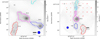 |
Fig. B.1 1.39 mm continuum emission, toward region F2 (left panel) and region F3 (right panel), in contours that depict [10, 20, 30, 40, 50, 60, 70, 80, 90, 100, 150, 300, 500, and 700] times the rms noise (0.12 mJy beam−1), overlapped with magnetic field segments in blue, where thin and thick segments depict segments within the inner 50% and 40% of the primary beam model, respectively. At 350 μm, the red segments show the CSO magnetic field. The thin segments have a polarization intensity between two and three sigmas, and the thick segments have an intensity greater than three times sigma (CSO sigma =0.02 Jybeam−1 Añez-López et al. 2020). Color contours show leaves from dendrogram analysis, also black label present the corresponding ID label. Blue solid circle depict the ALMA beam size. The Pink triangle shows the H2 O maser detected in Wang et al. (2006). Yellow tripods depict radio sources detected at 6 cm (C-band) by Díaz-Márquez et al. (2024). White tripods show NH3 cores detected by Ohashi et al. (2016). |
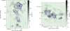 |
Fig. C.1 Local gravity normalized vectors overlapped with magnetic field. |
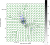 |
Fig. C.2 Local gravity normalized vectors |
Appendix D Polarization fraction
In this section we present the maps that display the percentage of polarization detected toward the N, S and F1 regions (see Fig. D.1).
Appendix E Structure function
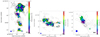 |
Fig. D.1 Polarization fraction in colors overlapped with continuum emission in contours. |
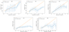 |
Fig. E.1 Structure functions and fits for regions N2, N4, N5, N7, and N8, where fittings are for l<1.5. The separation is expressed in terms of the beam size. Error bars are the standard deviations of angle differences at a given distance. The fitted intercepts are 9.5°, 17.2°, 17.1°, 53.4° and 48.1°, respectively. |
 |
Fig. E.2 Structure functions and fits for regions S2, S3, S6, and S8, where fittings are for l<1.5. The separation is expressed in terms of the beam size. Error bars are the standard deviations of angle differences at a given distance. The fitted intercepts are 26.9°, 65.2°, 31.7°, and 57.7°, respectively. |
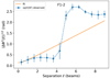 |
Fig. E.3 Structure functions and fits for regions F1-2, where fittings are for l<1.5. The separation is expressed in terms of the beam size. Error bars are the standard deviations of angle differences at a given distance. The fitted intercept is 15°. |
All Tables
All Figures
|
Fig. 1 CSO continuum emission at 350 μm (gray map) and red contours, which depict [3, 6, 9, 15, 25, 35, 45, 55, 65, 75, 85, and 95] times the rms noise (80 mJy beam−1). The red and black circles in the lower left corner show the CSO and ALMA beam size, respectively. Blue contours represent the 80%, 40%, and 33% levels of the ALMA primary beam for each target region, labeled N, F1, F2, F3, and S. |
| In the text | |
|
Fig. 2 Continuum emission at 1.39 mm toward region N (upper panel) and region S (bottom panel). Contours depict [10, 20, 30, 40, 50, 60, 70, 80, 90, 100, 150, 300, 500, and 700] times the rms noise (0.12 mJy beam−1), overlapped with magnetic field segments in blue, where thin and thick segments depict segments within the inner 50% and 40% of the primary beam model, respectively. Red segments show the CSO magnetic field at 350 μm, where thin and thick segments indicate a polarization intensity between two and three sigmas and higher than three times sigma, respectively (CSO sigma =0.02 Jybeam−1 Añez-López et al. 2020). Color contours show the leaves from the dendrogram analysis, while the black labels present the corresponding ID label. The blue solid circle in the bottom left corner of each panel depict the ALMA beam size. The pink triangle shows the H2 O maser detected in Wang et al. (2006). Green tripods show cores detected with the SMA telescope at 1.3 mm (Busquet et al. 2016). Yellow and purple tripods depict radio sources detected at 6 cm (C-band) and at 3.6 cm (X-band) by Díaz-Márquez et al. (2024), respectively. White tripods show NH3 cores detected by Ohashi et al. (2016). |
| In the text | |
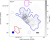 |
Fig. 3 Same as Fig. 2-left, but for region F1. |
| In the text | |
|
Fig. 4 Magnetic field position angle histogram toward region N (top) and S (bottom). Black solid lines depict the angle median value i.e., 95° for region N and (44°, 153°) for region S. Red dotted lines show the main direction of the CSO magnetic field orientation, 105° and (33°, 134°) for regions N and S, respectively, as shown in Añez-López et al. (2020). Magenta dashed line is set perpendicular to the main filament orientation (i.e., F10-E, 100°, Busquet et al. 2013). Magenta solid and dotted lines indicate the overall orientation of the polarization in the H and R bands, respectively (Santos et al. 2016). |
| In the text | |
|
Fig. 5 Magnetic field position angle histogram, toward region F1. Black solid line depicts the median value over the distribution (∼ 26°). Magenta dashed lined shows the orientation of main filament orientation (∼ 10°) Busquet et al. (2013). Magenta solid and dotted lines indicate the overall orientation of the polarization in the H and R bands, respectively (Santos et al. 2016). |
| In the text | |
|
Fig. 6 Relative position angle map and histogram (left and right, respectively) of the magnetic field observed by current ALMA ∼ 2′′ ar and by former CSO ∼ 10′′ ar toward region N (upper) and S (bottom). |
| In the text | |
|
Fig. 7 ΣB map in color toward region N. Black and colored contours show the Stokes I and the leaves found via the dendrogram analysis. |
| In the text | |
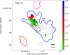 |
Fig. 8 Similar to Fig. 7, but for region F1. |
| In the text | |
|
Fig. 9 Median distortion of the magnetic field as a function of the averaged number density computed for each individual condensation in both Hub-N and Hub-S, shown by the blue stars and red squares, respectively. |
| In the text | |
|
Fig. B.1 1.39 mm continuum emission, toward region F2 (left panel) and region F3 (right panel), in contours that depict [10, 20, 30, 40, 50, 60, 70, 80, 90, 100, 150, 300, 500, and 700] times the rms noise (0.12 mJy beam−1), overlapped with magnetic field segments in blue, where thin and thick segments depict segments within the inner 50% and 40% of the primary beam model, respectively. At 350 μm, the red segments show the CSO magnetic field. The thin segments have a polarization intensity between two and three sigmas, and the thick segments have an intensity greater than three times sigma (CSO sigma =0.02 Jybeam−1 Añez-López et al. 2020). Color contours show leaves from dendrogram analysis, also black label present the corresponding ID label. Blue solid circle depict the ALMA beam size. The Pink triangle shows the H2 O maser detected in Wang et al. (2006). Yellow tripods depict radio sources detected at 6 cm (C-band) by Díaz-Márquez et al. (2024). White tripods show NH3 cores detected by Ohashi et al. (2016). |
| In the text | |
|
Fig. C.1 Local gravity normalized vectors overlapped with magnetic field. |
| In the text | |
|
Fig. C.2 Local gravity normalized vectors |
| In the text | |
|
Fig. D.1 Polarization fraction in colors overlapped with continuum emission in contours. |
| In the text | |
|
Fig. E.1 Structure functions and fits for regions N2, N4, N5, N7, and N8, where fittings are for l<1.5. The separation is expressed in terms of the beam size. Error bars are the standard deviations of angle differences at a given distance. The fitted intercepts are 9.5°, 17.2°, 17.1°, 53.4° and 48.1°, respectively. |
| In the text | |
|
Fig. E.2 Structure functions and fits for regions S2, S3, S6, and S8, where fittings are for l<1.5. The separation is expressed in terms of the beam size. Error bars are the standard deviations of angle differences at a given distance. The fitted intercepts are 26.9°, 65.2°, 31.7°, and 57.7°, respectively. |
| In the text | |
|
Fig. E.3 Structure functions and fits for regions F1-2, where fittings are for l<1.5. The separation is expressed in terms of the beam size. Error bars are the standard deviations of angle differences at a given distance. The fitted intercept is 15°. |
| In the text | |
Current usage metrics show cumulative count of Article Views (full-text article views including HTML views, PDF and ePub downloads, according to the available data) and Abstracts Views on Vision4Press platform.
Data correspond to usage on the plateform after 2015. The current usage metrics is available 48-96 hours after online publication and is updated daily on week days.
Initial download of the metrics may take a while.