| Issue |
A&A
Volume 707, March 2026
|
|
|---|---|---|
| Article Number | A331 | |
| Number of page(s) | 17 | |
| Section | Interstellar and circumstellar matter | |
| DOI | https://doi.org/10.1051/0004-6361/202556930 | |
| Published online | 20 March 2026 | |
A study of four multipolar planetary nebulae in the Galactic bulge
1
College of Geoexploration Science and Technology, Jilin University,
Changchun
130061,
China
2
Institute of Integrated Information for Mineral Resources Prediction, Jilin University,
Changchun
130061,
China
3
Laboratory for Space Research, Faculty of Science, The University of Hong Kong,
Hong Kong,
China
4
École Polytechnique,
91128
Palaiseau cedex,
France
5
Institute of Geochemistry, Chinese Academy of Sciences,
Guiyang
550081,
China
6
CAS Centre for Excellence in Comparative Planetology, Chinese Academy of Sciences,
Hefei
230026,
China
7
Lunar Exploration and Space Engineering Centre, China National Space Administration,
Beijing
100190,
China
★ Corresponding authors: This email address is being protected from spambots. You need JavaScript enabled to view it.
; This email address is being protected from spambots. You need JavaScript enabled to view it.
Received:
21
August
2025
Accepted:
27
January
2026
Abstract
We present infrared (IR) spectroscopic and optical morphological analyses of four multipolar young planetary nebulae (PNe) located in the Galactic bulge (GB) to investigate their dust characteristics and complex multi-lobed structures. Hubble Space Telescope high-resolution images of the nebulae (H 1-8, H 1-43, K 5-4, and M 3-14) reveal that these objects have interlaced multi-lobed features, indicating that their formation process is complex. Spitzer IR spectroscopic measurements of three of the young PNe show that these nebulae have unidentified IR emission bands and broad silicate features, suggesting the existence of a mixed-chemistry dust environment around these objects; such an environment, if present, may be caused by the last thermal pulse of the final asymptotic giant branch phase or be related to the thick tori produced by the interactions of central binaries. To find a potential connection between the multi-lobed shapes and central stars (CSs) of these nebulae, we employed Transiting Exoplanet Survey Satellite (TESS) monitoring to check whether the CSs of the objects exhibit photometric variations. Analysis of TESS observations of the four young PNe shows that the CS of H 1-43 exhibits a periodic photometric variation of 20.88 hr; no regular brightness variations are detected for the other three nebulae. To study and differentiate the multipolar nebulae in the Galactic disk (GD) and GB, a statistical analysis was performed on the properties of these nebulae. The binary fraction of multipolar PN CSs in the GD region is estimated to be 23-40%, which is significantly larger than the binary fraction of the PN CSs reported in other studies. This strongly supports the hypothesis that binary interactions play an important role in the formation of multipolar PNe. Analyses of the spectral energy distributions of the objects show that their IR luminosities, dust temperatures, and mean emission measures are higher than the averages for normal PNe, which may indicate that they are young.
Key words: stars: AGB and post-AGB / ISM: structure / infrared: ISM / planetary nebulae: individual: H 1-8 / planetary nebulae: individual: H 1-43 / planetary nebulae: individual: K 5-4
© The Authors 2026
 Open Access article, published by EDP Sciences, under the terms of the Creative Commons Attribution License (https://creativecommons.org/licenses/by/4.0), which permits unrestricted use, distribution, and reproduction in any medium, provided the original work is properly cited.
This article is published in open access under the Subscribe to Open model. This email address is being protected from spambots. You need JavaScript enabled to view it. to support open access publication.
1 Introduction
Planetary nebulae (PNe) are important objects for studying the final stages of the evolution of low- and medium-mass stars. During the asymptotic giant branch (AGB) and post-AGB stages, stars eject large amounts of material, which is then ionized by ultraviolet (UV) radiation from the central stars (CSs) and eventually forms PNe. With the advancement of high-angular-resolution and high-dynamic-range observation technology, especially through the James Webb Space Telescope (JWST) and Hubble Space Telescope (HST), some PNe have been revealed to have complex multipolar structures, rather than being limited to simple elliptical shells or bipolar morphologies (De Marco et al. 2022; Hsia et al. 2010, 2014, 2019; López et al. 1998; Manchado et al. 1996; Wen et al. 2023, 2024). Multipolar PNe usually show two or more pairs of axisymmetric structures, suggesting that the formation of this type of object involves high-speed, highly collimated outflows from different directions, or outflow directions that vary with time (Hsia et al. 2014). In addition, the vast majority of these objects are compact and fairly young, suggesting that multipolar PNe have a significant impact on the early stages of PN evolution (Wen et al. 2023; Hsia et al. 2014). Not many PNe with multipolar appearances have been discovered to date, due to low-resolution images or observations with poor dynamic ranges.
During the evolution of multipolar PNe, the shapes and structures of these objects vary with their CS evolution, the density variation of the surrounding environment, and different observation angles (Hsia et al. 2014). Multipolar young PNe (YPNe) usually show morphological diversity and structural complexity. Over the past two decades, there has been increasing interest in the properties of multipolar YPNe in the Galactic disk (GD), especially their complex nebular structures, chemical compositions, and ionized gas components (Hsia et al. 2014; Kwok & Su 2005; Sahai 2000; Sahai et al. 2011). Although several scenarios have been proposed to clarify the formation of multipolar nebulae (Avitan & Soker 2025; García-Segura et al. 2006; García-Segura 2010; López et al. 1995; Steffen et al. 2013; Velázquez et al. 2012), the exact mechanism responsible for the multi-lobed structures of these objects remains unclear. In the late AGB or post-AGB phase, binary and/or multiple substellar companion interactions or the precession of the rotation axis of the mass-loss star may be the key factors (García-Segura 1997, 2010; Hsia et al. 2014; Velázquez et al. 2012). Avitan & Soker (2025) suggest that the axis of one of the lobes of a multipolar PN is due to the orbital angular momentum of a binary system, and that the axis of the other lobe is caused by mighty envelope convection of the mass-losing massive progenitor star. Observations using high-resolution and high-sensitivity telescopes, especially next-generation telescopes, will be crucial to elucidating the physical processes involved in the formation and evolution of these multipolar YPNe. Such observations can help us obtain a deeper understanding of the progenitors of these objects in the late AGB or post-AGB phase (De Marco et al. 2022; Sahai et al. 2023).
Recent space-based all-sky photometric observations such as the Kepler Space Telescope and the Transiting Exoplanet Survey Satellite (TESS) have provided a new means for discovering the binary CSs of PNe (CSPNe; Handler et al. 2013; De Marco et al. 2015; Aller et al. 2020; Jacoby et al. 2021; Rechy-García et al. 2022; Wen et al. 2024). Through high-precision continuous photometric monitoring, the missions can effectively identify the potential periodic photometric variations in CSPNe due to binary interactions (Aller et al. 2020). With the retirement of the Kepler Space Telescope, TESS has become the best tool for searching for short-period binaries in PNe. A preliminary study of the eight Galactic CSPNe observed by TESS revealed that all but one show meaningful periodic variability, which may be caused by the central binary interactions of PNe (Aller et al. 2020). For multipolar PNe, the central binary interactions may be the key mechanism for forming the multipolar appearance of such objects. To find the possible connection between the CSs of multipolar YPNe and their multiple lobe-like structures, Wen et al. (2024) attempted to search for the existence of central binary stars in YPNe with a multipolar appearance. They found a nebula in the TESS observations that exhibited periodic photometric variations, which may be caused by the binary star in the core of the PN. However, the observed photometric variations of the CSPNe may still be contaminated by nearby sources around the nebulae (Aller et al. 2020; Wen et al. 2024). These studies suggest that TESS observations can open up another avenue for searching for central binaries of multipolar YPNe.
Compared with the GD and halo regions, the origin and evolution of the Galactic bulge (GB) remain poorly resolved. It is generally believed that the GB is a region at the center of our Milky Way galaxy composed of many old stars (≥10 Gyr; Nataf 2016). Subsequent studies (Bensby et al. 2013; Gesicki et al. 2014; Nataf 2016) suggested that the GB contains two different stellar populations: one that is old and metal-poor and one that is young and metal-rich (bulge AGB stars and PNe). Infrared (IR) spectroscopic surveys of some GB PNe have shown that most nebulae in the sample exhibit the signature of a mixed dust chemistry (Perea-Calderón et al. 2009; Stanghellini et al. 2012), which could be due to a final thermal pulse at the end of AGB phase (or after) causing the object to transition from O-rich to C-rich (Perea-Calderón et al. 2009), or due to the photodissociation of a thick torus associated with the central binary (Guzman-Ramirez et al. 2011, 2014). Tan et al. (2023b) conducted a series of statistical analyses on 136 GB PNe and found that 68% of the objects in their sample are bipolar in shape. They also found 14 GB PNe that host short-period binaries (they are almost bipolar nebulae), whose major axes are almost parallel to the Galactic plane. In fact, multipolar PNe are often misclassified as bipolar (B) or elliptical (E) nebulae (Hsia et al. 2010, 2014). Past studies of multipolar nebulae have mostly focused on such objects in the GD (Hsia et al. 2010, 2014, 2019; Sahai et al. 2011; Wen et al. 2024), while information on the chemical compositions, dust properties, and structural distributions of these nebulae located in the GB is still relatively lacking. Therefore, studying multipolar PNe in the GB can not only provide important information about the relationship between nebular morphology and the characteristics of their central sources, but also reveal the influence of their surrounding environments in shaping the morphology of these objects. Such further works can increase our understanding of the evolution of the GB and enhance our exploration of the last phase of the evolution of medium- and low-mass stars.
To search for more multipolar PNe in the GB and study their properties, we reexamined a sample of 40 compact bulge PNe observed by HST in Tan et al. (2023a). The high-resolution HST images resolve the multipolar shapes and intrinsic complex structures of these objects well. Four nebulae (H 1-8, H 1-43, K 5-4, and M 3-14) were selected from the sample based on the following criteria: (i) these objects appear as multipolar shapes (including nested ones) in the HST images; (ii) the nebulae have been observed by the TESS mission in a search for their central binaries; and/or (iii) their IR spectra show mixed dust chemistry signatures.
In this study, we performed a multiwavelength investigation of four multipolar PNe located in the GB based on HST optical images, Spitzer mid-IR (MIR) spectral data, and TESS photometric observations. We explored the spatial structure distribution, dust properties, and chemical composition of these four nebulae, as well as their interactions with the surrounding environment. Section 2 introduces the observational data of these nebulae, including optical photometry, MIR spectral observations, and optical images, as well as related data processing methods. The results of the individual observations are summarized in Sect. 3. In Sect. 4 we derive the properties of these four nebulae from the spectral energy distribution (SED). A comparison of the properties of multipolar YPNe in the GD and GB regions is presented in Sect. 5. In Sect. 6, we summarize our work.
2 Observation and data reduction
2.1 High-resolution HST optical imaging
Optical images of the PNe H 1-8, H 1-43, K 5-4, and M 3-14 presented in the study are obtained from the Mikulski Archive for Space Telescopes (MAST). To obtain images with high spatial resolution, all data were observed through the HST observing program ID 9356 (PI: A. Zijlstra) using the Planetary Camera (PC) of the Wide Field and Planetary Camera 2 (WFPC2). The field of view of the PC is ![Mathematical equation: $\[36^{\prime\prime}_\cdot 8 \times 36^{\prime\prime}_\cdot8\]$](/articles/aa/full_html/2026/03/aa56930-25/aa56930-25-eq1.png) (800 pixel × 800 pixel) and its image resolution is
(800 pixel × 800 pixel) and its image resolution is ![Mathematical equation: $\[0^{\prime\prime}_\cdot045\]$](/articles/aa/full_html/2026/03/aa56930-25/aa56930-25-eq2.png) per pixel. A narrowband Hα filter (F656N: λc = 6564 Å, Δλ = 22 Å) was used to capture the overall characteristics of these PNe and detailed imaging of the nebular structures. Total exposure time for each target was 200 s.
per pixel. A narrowband Hα filter (F656N: λc = 6564 Å, Δλ = 22 Å) was used to capture the overall characteristics of these PNe and detailed imaging of the nebular structures. Total exposure time for each target was 200 s.
To provide a reliable basis for subsequent morphological analysis, the raw science data were processed and calibrated using the Image Reduction and Analysis Facility (IRAF) STSDAS software package. Data reduction processes including flatfield correction, cosmic-ray removal, and bias calibration, were successfully performed and are important for reducing artifacts and noise in the images. The processed F656N (Hα) grayscale images of the four PNe are shown in Fig. 1 and a journal of the HST WFPC2 observations of the objects is summarized in Table A.1. These high-resolution images truly reveal the nebular structures and distributions of these objects.
2.2 TESS time-domain photometry
The TESS is an all-sky transit survey satellite that has scanned more than 93% of the sky. The satellite is equipped with four high-sensitivity wide-field cameras that can cover an area of 96° × 24° of the sky. The camera contains four 2K×2K CCD detectors, providing a spatial resolution of 21″ pixel−1. The long-term uninterrupted TESS observations (approximately 27 days) and its high-quality photometric data can provide a valuable opportunity to discover and study the periodic variations of the central binaries of multipolar nebulae.
The TESS photometric data for these four PNe (H 1-8, H 1-43, K 5-4, and M 3-14) were obtained from the MAST database. These nebulae were captured as full frame images at a cadence of 200 seconds. We downloaded the full frame image 15×15 pixel2 cutout images (![Mathematical equation: $\[5 ^{\prime}_\cdot 3{\times}5^{\prime}_\cdot3\]$](/articles/aa/full_html/2026/03/aa56930-25/aa56930-25-eq3.png) ) from MAST’s TESScut service to extract accurate photometric data of the CSPNe and then converted them into target pixel files (TPFs). A summary of the TESS observations is given in Table A.1 and the TPFs of the four nebulae are shown in Fig. 2.
) from MAST’s TESScut service to extract accurate photometric data of the CSPNe and then converted them into target pixel files (TPFs). A summary of the TESS observations is given in Table A.1 and the TPFs of the four nebulae are shown in Fig. 2.
Data processing, aperture selection, photometric measurement, light curve generation, elimination of low-frequency and long-term trends, and removal of anomalous data points were all performed using the same methods described by Wen et al. (2024). We employed a Lomb-Scargle periodogram analysis to search for potential periodic signals in the observed light curves measured at nonuniform intervals. Based on the period values determined in the periodograms, the corresponding phase-folded light curves of these nebulae were then created.
Due to the poor resolution of the TESS images (21″ pixels−1), we must be particularly careful when performing photometric analyses of the CSs in the nebulae. Other sources near the PNe may contaminate the observed photometric variations, leading us to misinterpret the observations (Higgins & Bell 2023; Pedersen & Bell 2023). Figure 2 shows how the photometry can be contaminated by a few nearby sources of comparable brightness to the target, making it more challenging to distinguish the contribution of the CSPN from the observations. To ensure that the photometric variations indeed originate from the CSs of the target nebulae and not from other nearby sources in the same apertures, two different checks were performed on individual CSPNe. The first step was to analyse the periodograms of the CSPNe using the TESS_Localize package, which can more accurately localize sources of variation to less than 20 percent of a TESS pixel (Higgins & Bell 2023). The same method as Wen et al. (2024) is then used to select the objects whose brightness actually varies. After our analysis using the TESS_Localize package, additional visual checks were performed on the TPFs created by this package to ensure that the locations of the objects matched those of the CSs in the nebulae.
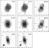 |
Fig. 1 HST gray Hα images of four multipolar YPNe with a logarithmic scale. Their corresponding images are also displayed but labeled with various structural features. The white crosses denote the locations of CSs. An inner torus (dotted orange line) at the waist of K 5-4 can be seen in the inset. |
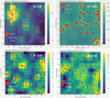 |
Fig. 2 TESS TPFs of four YPNe. The filled circles and black crosses denote the Gaia DR2 objects and the YPNe. The white grid areas overlaid on the TPF maps represent the apertures used to obtain the target fluxes. Photometry results of these nebulae may be contaminated by other objects within the same apertures. The electron-counting scale bars are presented on the right. |
2.3 Spitzer mid-infrared spectroscopy
The Spitzer Space Telescope is an IR space observatory equipped with an infrared spectrometer (IRS) and an infrared array camera, which can sensitively detect IR thermal radiation from various celestial objects. In this study, low- and medium-resolution Spitzer IRS spectra of three PNe (H 1-8, H 1-43, and K 5-4) were obtained through three programs 28561632 (PI: L. Stanghellini), 11325696 (PI: M. Bobrowsky), and 25861376 (PI: L. Stanghellini), respectively, to further understand their dust characteristics. The observations utilized four different modes of the Spitzer IRS instrument including the long-high (LH), long-low (LL), short-low (SL), and short-high (SH) modules, providing low (R~57–127) and medium (R~ 600) spectral resolution with total wavelength coverage from 5.2 to 39.8 μm. The slit sizes for LH, LL, SL, and SH modules are ![Mathematical equation: $\[22^{\prime \prime}_\cdot 3 \times 11^{\prime \prime}_\cdot 1, 168^{\prime \prime}{\times}10^{\prime\prime}_\cdot 7, 57^{\prime \prime}{\times}3^{\prime \prime}_\cdot7\]$](/articles/aa/full_html/2026/03/aa56930-25/aa56930-25-eq4.png) , and
, and ![Mathematical equation: $\[11^{\prime \prime}_\cdot 3{\times}4^{\prime \prime}_\cdot7\]$](/articles/aa/full_html/2026/03/aa56930-25/aa56930-25-eq5.png) , respectively. The apertures for the spectroscopic observations of H 1-8, H 1-43, and K 5-4 were set in the central parts of the objects, covering almost the entire nebulae to capture the maximum fluxes from the targets. Total exposures for the nebulae range from 40 to 218 s.
, respectively. The apertures for the spectroscopic observations of H 1-8, H 1-43, and K 5-4 were set in the central parts of the objects, covering almost the entire nebulae to capture the maximum fluxes from the targets. Total exposures for the nebulae range from 40 to 218 s.
We calibrated and reduced the MIR spectra of these compact PNe using Spitzer Science Centre (SSC) pipeline version s18.7 to ensure data quality and consistency. In the processing stage, anomalous pixels were first removed using the IRSCLEAN program and then the spectra of individual nebulae were extracted using the optimal extraction method in the Spectral Modelling and Reduction Tool (SMART) package (Higdon et al. 2004). To enhance the quality and reliability of the spectra, IRS spectroscopic measurements of these nebulae obtained from different exposures were combined to produce the final spectra.
It is noteworthy in these observations that the slit widths of the SL (![Mathematical equation: $\[3^{\prime\prime}_\cdot7\]$](/articles/aa/full_html/2026/03/aa56930-25/aa56930-25-eq6.png) ) and SH (
) and SH (![Mathematical equation: $\[4^{\prime\prime}_\cdot7\]$](/articles/aa/full_html/2026/03/aa56930-25/aa56930-25-eq7.png) ) modules are narrower than those of the LH (
) modules are narrower than those of the LH (![Mathematical equation: $\[11^{\prime\prime}_\cdot1\]$](/articles/aa/full_html/2026/03/aa56930-25/aa56930-25-eq8.png) ) and LL (
) and LL (![Mathematical equation: $\[10^{\prime\prime}_\cdot7\]$](/articles/aa/full_html/2026/03/aa56930-25/aa56930-25-eq9.png) ) modules, so the measurements using smaller apertures may result in flux losses during the observations. To address this issue, scaling corrections are performed on the SL or/and SH data of H 1-8, H 1-43 and K 5-4. We multiplied the SH and SL observations for H 1-43 by 1.26 and 1.23, and for K 5-4 by 1.75 and 1.15, respectively, to adjust the continuum intensities of the overlapping regions of the LH and SL/SH spectra to be consistent. For PN H 1-8, because the SL measurement used a smaller aperture than the LL data, the SL spectrum is multiplied by a factor of 1.18 to make the continuous emission levels consistent in the overlapping parts of the LL and SL spectra. The IRS observations of these compact PNe are summarized in Table A.2.
) modules, so the measurements using smaller apertures may result in flux losses during the observations. To address this issue, scaling corrections are performed on the SL or/and SH data of H 1-8, H 1-43 and K 5-4. We multiplied the SH and SL observations for H 1-43 by 1.26 and 1.23, and for K 5-4 by 1.75 and 1.15, respectively, to adjust the continuum intensities of the overlapping regions of the LH and SL/SH spectra to be consistent. For PN H 1-8, because the SL measurement used a smaller aperture than the LL data, the SL spectrum is multiplied by a factor of 1.18 to make the continuous emission levels consistent in the overlapping parts of the LL and SL spectra. The IRS observations of these compact PNe are summarized in Table A.2.
Although Spitzer spectroscopic observations of these three nebulae have been presented by Guzman-Ramirez et al. (2011) and Stanghellini et al. (2012), the nature and properties of dust components of the objects are not well investigated. We reexamined the IR spectra of the nebulae to further study their dust properties, unidentified infrared emission (UIE) bands, and broad silicate features.
Measurements of characteristic structures in HST images of the four YPNe.
3 Results
3.1 Morphological structures of individual nebulae
The four nebulae (H 1-8, H 1-43, K 5-4, and M 3-14) are thought to be YPNe because of their [O III] λ5007/Hα flux ratios smaller than 1 and their small sizes (Sahai et al. 2011). As can be seen from Fig. 1, the PN H 1-8, H 1-43, and M 3-14 show a multipolar appearance with multiple sub-lobes, while K 5-4 exhibits a nested hourglass shape, which can be considered an atypical multipolar nebula (Hsia et al. 2014; Wen et al. 2023). The nested bipolar structures seen in this nebula may be the result of (i) several episodic mass ejections from the central binary (Hsia et al. 2021), (ii) different ionization layers in the photodissociation region excited by far-UV radiation of the CS (Hsia et al. 2021), or (iii) ionization and heating of the gas in the lobe walls by fast stellar winds (Balick et al. 2022). In addition to the multipolar structures seen in these YPNe, some of them exhibit notable features including the tori around the waists and faint halos. The multipolar lobes and waist-shaped torus structures detected in the objects indicate that the processes that formed such YPNe are quite complex. The CSs are visible only in H 1-8, H 1-43, and M 3-14. To measure the orientations and diameters of the lobe structures of these YPNe, we fit ellipses to the shapes shown on the narrowband images. In this study, since the four nebulae are located in the dense regions of the GB, we cannot obtain their high-precision Gaia distance data. Instead, the distances to these YPNe can only be obtained from various literature. Table 1 lists the measured parameters of the observed structures, such as the position angle (PA) of the major axis, the size of the feature, and the derived tilt angle. The kinematic ages of these nebulae are estimated based on the physical diameters (derived from the conversion of the angular sizes and distances), nebular expansion velocities, and inclination angles of their longest lobes. For a multipolar PN, Guillén et al. (2013) find that the expansion velocities of their lobe-like structures are faster than that of other parts of the nebula. Therefore, given the relatively precise distances to these objects, the kinematic ages derived here are just upper limits. The kinematic ages of the four nebulae range from 1710 to 5930 yr (see text), which is consistent with previous conclusions that the kinematic ages of GB PNe are typically less than 6000 yr, and suggests that these nebulae are associated with a younger, more metallic bulge population (Gesicki et al. 2014). The structural descriptions of these YPNe are listed below.
3.1.1 H 1-8 (PN G352.6+03.0)
Parker et al. (2005) initially classified H 1-8 as an E-type nebula based on low-resolution SuperCOSMOS Hα survey images. According to the ERBIAS-sparm morphological classification proposed by Parker et al. (2006), the PN is further classified as a Bamprs nebula (Tan et al. 2023a). At first glance, the HST Hα image of the PN (Fig. 1) reveals a pair of large bipolar lobes (with a size of ![Mathematical equation: $\[4^{\prime \prime}_\cdot 44{\times}3^{\prime \prime}_\cdot04\]$](/articles/aa/full_html/2026/03/aa56930-25/aa56930-25-eq10.png) ) extending along the SW-NE direction (marked as lobe c − c′) and this structure dominates the nebula. The waist of this lobe has a large elliptical structure, which seems to be caused by the projection of the equatorial torus of the lobe c − c′. Assuming that the observed elliptical structure is formed by a tilted circular projection, the tilt angle of the structure is ~ 56° (the tilt angle of the sky plane is 0°), implying that the lobe c − c′ has the same tilt angle of 56±3° as the elliptical structure. When we further inspect the central part of H 1-8, we find that the nebula has two additional pairs of lobes (labeled lobes b − b′ and a − a′), which intersect roughly in the central region of the PN. An oval hollow shell structure (marked as d) with a size of
) extending along the SW-NE direction (marked as lobe c − c′) and this structure dominates the nebula. The waist of this lobe has a large elliptical structure, which seems to be caused by the projection of the equatorial torus of the lobe c − c′. Assuming that the observed elliptical structure is formed by a tilted circular projection, the tilt angle of the structure is ~ 56° (the tilt angle of the sky plane is 0°), implying that the lobe c − c′ has the same tilt angle of 56±3° as the elliptical structure. When we further inspect the central part of H 1-8, we find that the nebula has two additional pairs of lobes (labeled lobes b − b′ and a − a′), which intersect roughly in the central region of the PN. An oval hollow shell structure (marked as d) with a size of ![Mathematical equation: $\[1^{\prime \prime}_\cdot 44{\times}1^{\prime \prime}_\cdot05\]$](/articles/aa/full_html/2026/03/aa56930-25/aa56930-25-eq11.png) is visible in the central part of this nebula. This structure is probably the result of the projection of another bipolar lobe aligned almost along the line-of-sight direction, or a cavity formed by fast wind blowing from a central source. We can also detect similar structural features in other YPNe with a multipolar appearance, such as NGC 6644 (Hsia et al. 2010), M 1-59, M 1-61, and M 3-35 (Hsia et al. 2014).
is visible in the central part of this nebula. This structure is probably the result of the projection of another bipolar lobe aligned almost along the line-of-sight direction, or a cavity formed by fast wind blowing from a central source. We can also detect similar structural features in other YPNe with a multipolar appearance, such as NGC 6644 (Hsia et al. 2010), M 1-59, M 1-61, and M 3-35 (Hsia et al. 2014).
Adopting a distance of 8.98±1.8 kpc to this PN (Stanghellini & Haywood 2010), the physical size of lobe c − c′ is estimated to be 0.196±0.038 sec θ pc (θ is the inclination with respect to the sky plane). If we take the expansion velocity of H 1-8 to be the expansion velocity of most PNe with close central binaries (~25±12 km s−1; Jacob et al. 2013; Frew 2008) and an inclination angle of 56±3° for lobe c − c′, the kinematic age of this structure is derived to be ~3960±1920 yr based on the assumptions given above.
3.1.2 H 1-43 (PN G357.1-04.7)
Planetary nebula H 1-43 is classified as a bipolar nebula by Sahai et al. (2011) and a Bprs PN by Tan et al. (2023a), respectively, because this object primarily displays a pair of distinctly opposed lobes and also exhibits point-symmetric, ring-like, and internal streak structures. A careful inspection of Fig. 1 shows that H 1-43 exhibits a complex multipolar shape consisting of at least two pairs of different lobes (labeled lobes b − b′ and a − a′). Interestingly, the appearance of lobe a − a′ is roughly an S-shape with both ends closed, and its southern part twists toward the east and its northern part twists to the west. This structure can also be found in other nebulae with multipolar shapes such as Hen 2-73 (Wen et al. 2024) and Kn 26 (Guerrero et al. 2013), and may be caused by the crossing and overlapping of several pairs of multipolar lobes in the PNe (Chong et al. 2012) or by the binary precession of the CS (Hsia et al. 2014; Kwok & Su 2005). The central region of this object is a nearly circular shell-shaped cavity (marked as c) with a size of ![Mathematical equation: $\[0^{\prime\prime}_\cdot 61 {\times} 0^{\prime\prime}_\cdot55\]$](/articles/aa/full_html/2026/03/aa56930-25/aa56930-25-eq12.png) , which is similar to the structure seen in the central part of H 1-8. The central cavity of H 1-43 could be a projection of the third bipolar lobes almost along the line-of-sight direction, or a bubble blown out from a central source (Hsia et al. 2010, 2014). A faint, extended halo with an angular size of
, which is similar to the structure seen in the central part of H 1-8. The central cavity of H 1-43 could be a projection of the third bipolar lobes almost along the line-of-sight direction, or a bubble blown out from a central source (Hsia et al. 2010, 2014). A faint, extended halo with an angular size of ![Mathematical equation: $\[{\sim}3^{\prime \prime}_\cdot 3 {\times} 2^{\prime \prime}_\cdot5\]$](/articles/aa/full_html/2026/03/aa56930-25/aa56930-25-eq13.png) is also visible outside the main nebula (Fig. 1).
is also visible outside the main nebula (Fig. 1).
Adopting a distance of 8 kpc to H 1-43 (Tan et al. 2023a), we estimate the physical size of lobe a − a′ to be 0.104 sec θ pc (θ denotes the inclination to the sky plane). Assuming that the nebula expands at the same velocity as most PNe with close binary nuclei (~25±12 km s−1; Jacob et al. 2013; Frew 2008) and the tilt angle is 0° for lobe a − a′, the derived kinematic age of this structure is about 1710±760 yr. However, it is often found that the expansion velocity of a bipolar PN along the lobe direction is faster than that in other regions (Jacob et al. 2013). Taking into account the uncertainties in the lobe size measurements and the expansion velocity adopted due to the tilt effect in the 3D structures of the nebula, the derived kinematic age is only a rough estimate of one order of magnitude.
3.1.3 K 5-4 (PN G351.9-01.9)
Although K 5-4 is classified as a B-type YPN by Sahai et al. (2011) and a Bs nebula by Tan et al. (2023a), close examination of the HST images of this nebula (Fig. 1) reveals that the object has a nested shell-like appearance consisting of two closed bipolar lobes aligned in nearly the same direction (marked as lobes a − a′ and b − b′). The YPN with nested bipolar structures can also be observed in other objects such as M 2-9, Hb 12, Hen 2-320, (Hsia et al. 2014, 2010), and MyCn 18 (Miszalski et al. 2018). In addition, two ionized tori (marked as the “inner torus” and the “outer torus”) can be seen around the waist of the nebulae in the Hα image (see Fig. 1). From Table 1, we find that the major axes of two equatorial tori are almost along the same PA direction (PA = 97° and 102°) and they are nearly perpendicular to the axes of two bipolar lobes (PA = 9° and 12°). Assuming that the inner torus is perpendicular to the polar axes of two pairs of bipolar lobes and that this structure is formed by the projection of an inclined circle, the tilt angle of the inner torus is about 23±2° (the sky plane being 0°), corresponding to an inclination of 23±2° for this nebula. This result is consistent with the inclination value of 20° given by Gesicki et al. (2016) for the object.
Adopting 8 kpc as the distance to this YPN (Gesicki et al. 2016), the physical size of lobe a − a′ is about 0.213 s θ pc (where θ is the tilt angle between the sky plane and the major axis of the object). Assuming the expansion velocity of ~25±12 km s−1 (the expansion velocity of most PNe with close binary nuclei; Jacob et al. 2013; Frew 2008) and an inclination of 23±2° for this nebula, the kinematic age of this structure is estimated to be approximately 4320±2070 yr.
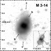 |
Fig. 3 VLT gray [O III] image of M 3-14 with various structures displayed on a logarithmic scale. Two distinct lobe-like structures (lobes b − b′ and c − c′) are visible in the VLT image, but lobe c − c′ cannot be found in the HST Hα image, as shown in the inset. |
3.1.4 M 3-14 (PN G355.4-02.4)
Sahai et al. (2011) and Tan et al. (2023a) classified M 3-14 as a B-type YPN and a Bms nebula, respectively, showing it to be a bipolar nebula with multiple shell structures and internal streaking features. The HST Hα image of M 3-14 (Fig. 1) shows that this nebula has a multipolar appearance similar to NGC 7026 (Clark et al. 2013), consisting of two pair of interlaced, closed bipolar lobes (marked as lobes b − b′ and a − a′). In addition to the observed multi-lobed structures, the object also has an ionized torus of size ![Mathematical equation: $\[5^{\prime \prime}_\cdot 63{\times}2^{\prime \prime}_\cdot78\]$](/articles/aa/full_html/2026/03/aa56930-25/aa56930-25-eq14.png) at its waist, whose major axis appears to be perpendicular to the major axis of the lobe b − b′ (see Table 1). Assuming that observed ionized torus is formed by the projection of an inclined circular plane, the tilt angle of this structure is ~ 29±3° (the inclination of the plane of the sky is 0°), which implies that the inclination angle of lobe b − b′ is 29±3°.
at its waist, whose major axis appears to be perpendicular to the major axis of the lobe b − b′ (see Table 1). Assuming that observed ionized torus is formed by the projection of an inclined circular plane, the tilt angle of this structure is ~ 29±3° (the inclination of the plane of the sky is 0°), which implies that the inclination angle of lobe b − b′ is 29±3°.
To search for the outer extended structure surrounding the nebula, we reexamined the Very Large Telescope (VLT) [O III] image of this object released by Tan et al. (2023a). Although this high-quality [O III] image has been previously presented by Tan et al. (2023a), the nature of these extended structures surrounding the YPN and their spatial distribution have not been studied. The VLT [O III] image of this object (Fig. 3) exhibits a multipolar appearance similar to that observed in HST Hα image. Compared with the HST Hα image, we can see the counterpart of lobe b − b′ in the VLT [O III] image, but not that of lobe a − a′. Interestingly, another pair of diffuse bipolar structures (masked as lobe c − c′) extending along the approximate N–S direction are observed only in the VLT [O III] image. The presence of these observed multiple lobes reflects the complex formation history of this YPN.
Adopting the distance of 6.47±1.6 kpc to M 3-14 (Zhang 1995), we derive the physical distance of lobe b − b′ to be ~0.297±0.073 sec θ pc. If we take the expansion velocity of K 5-4 as the expansion velocity of most PNe with close binary stars (about 25±12 km s−1; Jacob et al. 2013; Frew 2008) and the inclination of lobe b − b′ is 29±3°, a kinematic age of ~ 5930±2910 yr is derived for the structure based on these assumptions. If we take into account the uncertainties in the distance measurement and in the adopted expansion velocity of the nebula, the kinematic age derived here is only a preliminary estimate.
 |
Fig. 4 Observed TESS light curve (left panel), frequency power spectrum of the light curve (middle panel), and phase-binning (black) plus phase-folding (gray) light curves of H 1-43 (right panel). The black dots shown in the phase-binning light curve denote the average of the phase-folding curve data points, using the bin = 0.008 in phase. |
Results of the light curve analysis for the four YPNe.
3.2 Potential photometric variations of the nebulae
A series of inspections of the TESS data for these four CSPNe reveal that H 1-43 shows potentially periodic photometric variations, while H 1-8, K 5-4, and M 3-14 have no detectable regular brightness variations. The photometric light curve, frequency power spectrum of observed light curve, and phase-folded light curve plotted using the period derived from the light curve of H 1-43 are shown in Fig. 4. To highlight the observed photometric amplitude variations of the phase light curve, we also plot the binned phase-folded light curve (black dots) on the right panel of Fig. 4. The fitted periods and light curve analysis results of these four CSPNe is summarized in Table 2. Columns 1 and 2 give the names of the PNe and the fitted period. Columns 3 and 4 list the amplitude of the light curve and the time (T0) when the light curve modulation flux is minimum. The classification of periodic photometric variation according to the phase-folding curve shape is given in Col. 5. Columns 6 and 7 give the shapes of the PNe and the “relative likelihood” (RL) values obtained after the TESS_Localize check. The photometric variation results of these PNe are summarized below.
3.2.1 No regular photometric variation
Although these three nebulae (H 1-8, K 5-4, and M 3-14) exhibit multipolar shapes, information on photometric variations of the CSPNe and their IR excess due to the possible presence of cool companions has not been reported before. Compared to the CS of H 1-43, perhaps because these three CSPNe are fainter (see Table A.1) and contaminated by neighboring stars in the same apertures (Fig. 2), our current TESS analysis of the objects does not show any periodic photometric variations. Due to the limited observation time for these three targets, we cannot completely rule out the possibility that their CSPNe are long-period variable stars. Long-term photometric monitoring of the CSs of these three objects is needed to further confirm their true status.
3.2.2 New binary candidate: H 1-43
According to previous literature, there is no data showing that the CS of H 1-43 exhibits photometric variations. From the observed CS light curve of H 1-43 (top panel of Fig. 4), it can be seen that this object has photometric variations. By analyzing the frequency-power spectrum of the TESS data (left panel of Fig. 4), we can find a significant peak at a period of about 1.149 day−1 (20.88 h). The results of TESS_Localize analysis show that the detected frequency is truly from H 1-43 (with an RL value of about 96.34%), indicating that the reliability of this signal source is quite high. In the same aperture, the contamination effects from the other four sources (Gaia DR2 4042380853446223872 with RL = 1.92%, Gaia DR2 4042380853446257664 with RL = 1.13%, Gaia DR2 4042380853446242176 with RL = 0.51%, and Gaia DR2 4042380819086474240 with RL = 0.07%) are quite small. The Gaia distances of these four stars are 6.82 kpc, 9.67 kpc, 1.14 kpc, and 5.16 kpc for Gaia DR2 4042380853446223872, Gaia DR2 4042380853446257664, Gaia DR2 4042380853446242176, and Gaia DR2 4042380819086474240 (Khalatyan et al. 2024). The de-reddened colors (BP − RP)0 of Gaia DR2 4042380853446223872, Gaia DR2 4042380853446257664, Gaia DR2 4042380853446242176, and Gaia DR2 4042380819086474240 are −0.09 mag, 1.95 mag, 0.79 mag, and 1.19 mag (Khalatyan et al. 2024). In addition, subsequent visual check of the TPF image shows that the position of the frequency source obtained by the TESS_Localize analysis is consistent with the actual location of the observed CSPN, indicating that the source of photometric variation is likely from H 1-43 rather than from other nearby stars. This is the first time that the photometric variability of this CSPN is detected in the nebula. The CS phase-folding light curve of H 1-43 has a period of 20.88 hr and a low amplitude of about 0.12%. The curve of this nebula (the right panel of Fig. 5) is sinusoidal and similar in shape to CS light curves seen in other PNe, such as PHR J1713-2957, PHR J1724-2302, and Y-C 2-32 (Jacoby et al. 2021), which may be caused by the irradiation from a cool companion star (Retter et al. 1999; Jacoby et al. 2021).
Although the CS of H 1-43 shows periodic variations (even with RL value of ~ 96%), the photometric variability is likely to be contaminated by a few sources within the aperture that are similar in brightness to the CSPN (see Fig. 2), making it difficult to remove the contribution of these sources. Therefore, determining the exact origin of variations in this object is not straightforward. Long-term, high-resolution photometric observations are needed to help identify the true sources of these variations.
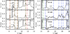 |
Fig. 5 Spitzer continuum-subtracted spectra of H 1-8, H 1-43, and K 5-4 in wavelength ranges from 5 to 14 μm and 15 to 35 μm. Prominent forbidden lines and H I features are marked. Dotted red, blue, and green lines indicate the positions of the UIE bands (6.2, 7.7, 8.6, 11.2/11.3, and 11.8 μm), broad silicate features at 18.0, 23.7, 27.6, 29.6, 30.6, 32.8, and 34.1 μm (Molster et al. 2002), and expected positions of prominent PAH bands (6.2, 7.7, 8.7, 11.2-11.3, and 16.4 μm; Sadjadi et al. 2015), respectively. |
3.3 Dust characteristics of the four multipolar nebulae
To better realize the nature and chemistry of the dust components of these YPNe, we examined their MIR spectra in detail, focusing on the silicate bands and UIE features. We applied fourth-order polynomials to fit the dust continuum components of these PNe and subtracted the fitted dust contributions from the observed spectra to highlight the studied spectral features. Since there is no spectral information for M 3-14, the residual Spitzer IRS spectra of the other three YPNe (H 1-8, H 1-43, and K 5-4) are shown in Fig. 5.
From Fig. 5, the prominent spectral features in the residual IR spectra are the forbidden emissions such as [Ar II] at 6.99 μm, [Na III] at 7.32 μm, [Ar III] at 8.99 and 21.83 μm, [S IV] at 10.51 μm, [Ne II] at 12.81 μm, [Ne III] at 15.56 μm, [S III] at 18.71 and 33.48 μm. Additionally, the obvious H I emissions at 12.37 and 7.46 μm can be seen in the IRS spectra of these YPNe.
The resulting IRS spectra of the three nebulae shown in Fig. 5 reveal several prominent UIE bands at 11.8, 11.2/11.3, 8.6, 7.7, and 6.2 μm. The UIE bands are usually attributed to polycyclic aromatic hydrocarbons (PAHs), which can be considered as an amorphous carbon solid (Li & Draine 2012; Kwok & Zhang 2013). In addition, we also see some silicate features at 18.0, 23.7, 27.6, 29.6, 30.6, 32.8, and 34.1 μm (Molster et al. 2002) in the long-wavelength part of the spectra, which are stronger than other weak silicate bands in the 33, 28, 23, and 18 μm complexes. The presence of UIE and silicate feature indicates that these three YPNe have a mixed chemical environment consisting of oxygen and carbon dust, which is common in dust types of other multipolar nebulae (Hsia et al. 2014). For the PN K 5-4, although we do not detect any photometric variations in this CSPN, the mixed chemistry displayed by the PN may be related to the dense torus structures at the waist of the nebula, probably produced by the interaction of the central binary of this object (Guzman-Ramirez et al. 2011, 2014). To further study the chemical composition distribution of the nebula (K 5-4) and its relationship with the CS, a series of high-spatial-resolution IR spectroscopic observations and long-term, high-sensitivity photometric monitoring for this YPN are needed.
4 Spectral energy distribution
The SED has long been recognized as a useful scientific method for analyzing various components of the YPNe (Zhang & Kwok 1991; Hsia et al. 2014, 2019, 2021). To better study different components (nebular, dust, and photospheric) of these nebulae (H 1-8, H 1-43, K 5-4, and M 3-14), we constructed four SEDs of the objects (Fig. 6), which cover wavelength coverage from 0.1 μm to 100 cm. In Fig. 6, the optical Panoramic Survey Telescope and Rapid Response System (Pan-STARRS), SkyMapper Southern Survey (SMSS), Sloan Digital Sky Survey (SDSS), and visual U, B, V, R, and I photometry of the four YPNe are taken from Chambers et al. (2016), Onken et al. (2024), and Gaia Collaboration (2022). MIR and near-IR photometric data were obtained from Herschel, Infrared Astronomical Satellite (IRAS), AKARI, Midcourse Space Experiment (MSX), Deep Near-Infrared Survey of the Southern Sky (DENIS), and Two Micron All Sky Survey (2MASS) catalogs, respectively. Furthermore, we added Wide-field Infrared Survey Explorer (WISE) and Spitzer photometric data of these YPNe following the same procedure described in Hsia & Zhang (2014). The color- and aperture-calibrations for WISE and Spitzer photometry are performed using the coefficients presented in Wright et al. (2010) and Reach et al. (2005). A journal of the photometric fluxes obtained from various observations is given in Table A.3. The IRS spectra of H 1-8, H 1-43, and K 5-4 are also plotted in Fig. 6. Since the nebulae are located in the GB and close to star-dense regions (see Fig. 2), their photometric results may be contaminated by nearby stars around the objects. After a series of detailed examinations of these four YPNe, we find that their far-IR and radio photometry are not contaminated by nearby stars. The MIR, visible, and NIR photometric contamination of the YPNe is estimated to be less than 15%, 35%, and 8%, respectively, which has a rather small impact on our results.
Figure 6 shows that a large portion of the total energies of these nebulae is emitted from the IR dust component, which is similar to what we have observed in the SEDs of other multipolar nebulae (Hsia et al. 2014, 2019; Wen et al. 2023, 2024). From Fig. 6, we can see that the emerging fluxes of the nebulae are fitted by two separate components including the gaseous nebular emission and reddened photospheric component (emitted from the central source) plus the dust thermal continuum. The proportion distributions of different components of four YPNe can be evidently identified. To fit the total observed fluxes of the four YPNe, we constructed a model consisting of the above components applying the same procedures described by Hsia et al. (2019). For the far-IR to MIR range of observed SEDs, the continuum curves are too wide to be fitted by the dust component alone. Therefore, we fit the observed SED curves using the DUSTY radiative transfer code (Ivezic & Elitzur 1997; Ivezic, Nenkova, & Elitzur 1999). In the fitting, the dust particle chemical composition is set to a mixture of silicate grains and amorphous carbon particles. The particle size follows the standard MRN distribution (Mathis, Rumpl, & Nordsieck 1977).
The model parameters used in these four nebulae and their comparison with normal PNe are shown in Table 3, where normal PNe represent hydrogen-rich nebulae and most PNe belong to this type (Muthumariappan & Parthasarathy 2020). The object names of these nebulae are listed in Col. 1. Columns 2 and 3 give the best approximation of central core effective temperatures (T*) and the values obtained from other literature (T*,ref) for comparison. The dust component temperatures (Td) and adopted optical depths at 0.7 μm (τ0.7) are given in Cols. 4–5. Columns 6 and 7 list dust chemical compositions used in the models and the adopted distances (D). The derived IR luminosities (LIR) of these PNe are listed in Col. 8. The LIR of the objects are obtained using the integrated fluxes of the dust component curves above 3 μm. Columns 9–12 give the masses of dust (Md) and nebular gas (Mg) components, dust-to-gas mass ratios (Md/Mg), and physical diameters, respectively. The masses of dust and gas components are estimated using the formulas described in Stasińska & Szczerba (1999). Various nebular parameters of the four PNe are taken from different literature sources. The electron temperatures and electron densities are taken from Chiappini et al. (2009) and García-Hernández & Górny (2014). Reddening-corrected Hβ line fluxes of the nebulae are derived from Acker et al. (1992) and Tylenda (1992). The dust emissivity index (α) and dust absorption coefficient of amorphous carbon at ![Mathematical equation: $\[60 ~\mu \mathrm{m}\left(K_{60}^{a b s}\right)\]$](/articles/aa/full_html/2026/03/aa56930-25/aa56930-25-eq15.png) are assumed to be 1 and 74.38 cm2 g−1 (Stasińska & Szczerba 1999), respectively, which better fits the dust chemistry we observe, since the IR spectral features of these nebulae are mainly dominated by UIE signatures (see Sect. 3.3). The errors of LIR, Md, Mg, and Md/Mg for the four nebulae are estimated through the errors in the various parameters used in the derivation of these physical quantities (LIR, Md, Mg, and Md/Mg), which are mainly dominated by the distance errors. The physical diameters of these YPNe (R) are derived based on the angular sizes of their longest axis and their distances from the literature. Although the results obtained through the fitting cannot fully reveal the true state of the four nebulae, we can still get good approximations by fitting the available photometric points.
are assumed to be 1 and 74.38 cm2 g−1 (Stasińska & Szczerba 1999), respectively, which better fits the dust chemistry we observe, since the IR spectral features of these nebulae are mainly dominated by UIE signatures (see Sect. 3.3). The errors of LIR, Md, Mg, and Md/Mg for the four nebulae are estimated through the errors in the various parameters used in the derivation of these physical quantities (LIR, Md, Mg, and Md/Mg), which are mainly dominated by the distance errors. The physical diameters of these YPNe (R) are derived based on the angular sizes of their longest axis and their distances from the literature. Although the results obtained through the fitting cannot fully reveal the true state of the four nebulae, we can still get good approximations by fitting the available photometric points.
As can be seen from Table 3, our approximation for the central core effective temperatures of these nebulae (T*) agrees well with the results previously reported in the literature (T*,ref). We also find that Td and LIR of these nebulae are higher than the average for normal PNe, and their physical diameters are smaller than the mean size of Galactic PNe. Furthermore, the mean emission measure (<EM>) of the four objects can be estimated based on the radio flux density measured at 3 GHz (almost optically thin) and the angular size of the radio emitting area at that frequency (Kwok et al. 1981; Umana et al. 2004). After some calculations, we found that the <EM> values of these nebulae are higher than 106 cm−6 pc, which lies within the <EM> coverage of known YPNe (~ 106–108 cm−6 pc; Umana et al. 2004). The results (high Td, LIR, and <EM>, and small physical sizes) may indicate that these four objects are relatively young compared to normal PNe (Stasińska & Szczerba 1999; Muthumariappan & Parthasarathy 2020). This may be because a PN expands with age, and the dust grains gradually move away from the central source, resulting in less radiation received by the dust component, which in turn causes the Td and LIR of the nebula to decrease (Stasińska & Szczerba 1999; Muthumariappan & Parthasarathy 2020). It is worth noting that the dust masses of the four nebulae we studied (particularly H 1-8 and M 3-14) are higher than the average for normal PNe. The result may indicate that the dust particles undergo destruction, fragmentation, or inter-particle collisions as PNe evolve (Lenzuni et al. 1989). However, some recent observations show that dust destruction process in PNe may not be as efficient as generally thought (Volk et al. 1997; Stasińska & Szczerba 1999), leaving the issue of dust survival in such nebulae still unsolved. Similar to the average Md/Mg value of normal PNe, we find that the Md/Mg values of the sample nebulae studied are roughly distributed in the range of 10−2 to 10−3, which is consistent with previous results (Stasińska & Szczerba 1999; Hsia et al. 2014; Muthumariappan & Parthasarathy 2020). There is no significant difference in Md/Mg between the two types of PNe (see Table 3), indicating that these values have no correlation with the age of these nebulae (Stasińska & Szczerba 1999; Muthumariappan & Parthasarathy 2020).
In addition, the physical diameters and kinematic ages of these four objects are similar to those of ten GD young multipolar nebulae (physical size ranges from 0.07 to 0.22 pc and the kinematic age ranges from ~1400 to 4800 yr) studied by Hsia et al. (2014) and another 66 multipolar or bipolar YPNe (with physical diameters ranging from 0.02 to 0.32 pc) proposed by Sahai et al. (2011). The CS masses of the multipolar YPNe can be derived by comparing their positions on the Hertzsprung-Russell diagram with the theoretical post-AGB evolutionary tracks at Z = 0.016 calculated by Vassiliadis & Wood (1994). To estimate the masses of the two sets of multipolar YPN CSs (four GB nebulae proposed in this study and ten GD objects previously studied), we obtained their T* and luminosities from different literature (Stasińska & Tylenda 1990; Mal’Kov 1997; Cazetta & Maciel 2000; Gesicki et al. 2006; Gesicki & Zijlstra 2007; Gesicki et al. 2014; Hsia et al. 2014). Based on their positions on the Hertzsprung-Russell diagram, the core masses of these multipolar nebulae are approximately no more than 0.633 M⊙.
Based on the photometric measurements of the three YPNe (H 1-8, H 1-43, and K 5-4) in the WISE 12 and 22 μm bands, their Spitzer 8 μm and 24 μm fluxes can be estimated using the empirical flux ratios of WISE 12 μm/Spitzer 8 μm and WISE 22 μm/Spitzer 24 μm obtained by Jarrett et al. (2013). Using photometric measurements obtained from AKARI and Herschel catalogs (9, 18, 100, and 160 μm bands) and the fluxes derived from Spitzer 8 μm and 24 μm bands, we estimate the dust fraction of PAHs (PAH mass fraction, qPAH) in these nebulae to be no more than 0.47% based on Tables 4–6 in Draine & Li (2007). Previous studies have shown that the ratio of UIE 7.7 μm band strength to total IR energy (I7.7/IIR) in PNe increases with increasing gas-phase C/O abundance ratio (Cohen & Barlow 2005). To estimate the gas-phase C/O abundance ratios of the three YPNe, we derived the C/O values of these nebulae (C/O = 0.35 for H 1-8, C/O = 0.59 for H 1-43, and C/O = 0.21 for K 5-4) using the regression line relationship between I7.7/IIR and nebular C/O ratio plotted in Fig. 3 of Cohen & Barlow (2005).
Our TESS photometric observations and current SED analysis reveal the presence of a central binary in the core of H 1-43, which may support the hypothesis that the appearance of the multi-lobed structures is related to the central binary of this YPN (García-Segura 2010; Velázquez et al. 2012). For H 1-8 and M 3-14, although the contributions of cool companions can be separated from the SED fits of these nebulae, we cannot detect the presence of cool companions with the current TESS observations due to the lack of long-term and high-dynamic range photometric observations. Deep observations of the CSs of these PNe using high-resolution spectroscopic measurements in the UV to near-IR range could help clarify such issues (Aller et al. 2015).
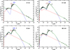 |
Fig. 6 SEDs of four YPNe from 0.1 μm to 100 cm. Available radio data are shown as filled rhombuses, Herschel photometry as crosses, WISE detections as open diamonds, IRAS photometric measurements as filled circles, MSX results as open rhombuses, SMSS u-, v-, g-, r-, i-, and z-band measurements plus other optical photometric data as open squares, AKARI photometry as asterisks, 2MASS results as open triangles, and DENIS data as filled triangles. The IRS spectra of three nebulae (H 1-8, H 1-43, and K 5-4) are also plotted. The UIE features at 6.2, 7.7, and 11.2 μm and several silicate bands at 23,28, and 33 μm can be seen in the fits. Note that some 12, 60, and 100 μm IRAS measurement results are upper limits. The green, blue, and red curves represent the total fluxes of all components, the best-fit values estimated using the DUSTY radiation transfer model (Ivezic, Nenkova, & Elitzur 1999), and the nebular contributions, respectively. |
Parameters adopted for the four YPNe.
5 Comparison of multipolar nebulae in the Galactic disk and bulge
For a long time, we have known little about the formation of multipolar YPNe in the GD and GB and their dust properties. The dust properties and chemical abundances of Galactic PNe may be related to the state of their CSs (García-Hernández & Górny 2014). Multipolar YPNe belong to a subclass of young nebulae. It would be interesting to investigate whether the appearances of multipolar YPNe in the GD and GB are related to their dust properties and CSs. To achieve this goal, we collected a large sample of 190 compact Galactic YPNe observed by HST (including 136 GD objects and 54 GB nebulae) from various literature sources (Sahai et al. 2011; Stanghellini et al. 2016; Tan et al. 2023b) and listed their properties (morphology, CS binarity, and dust type) in Table B.1. In the past, due to limitations in image resolution or dynamic range, the morphological classification of many multipolar YPNe was inaccurate. Now, images taken by the HST can clearly reveal the complex multi-lobed structures of this type of nebula. Therefore, we reexamined HST images of 190 existing nebulae in the sample and reclassified them using the main classes “ERBIAS” in morphological classification system (Parker et al. 2006) plus another extended class “M” (multipolar). In this study, we noticed that 73 of the 190 YPNe (~38%) were previously classified as belonging to the “B” or “E” classes, but these 73 nebulae have now been reclassified as belonging to the “M” class. The result clearly demonstrates that we have underestimated the number of multipolar nebulae in the past. This may be because early studies did not pay sufficient attention to the multi-lobed structures inside these objects, leading to misclassifications of their morphology.
As can been seen from Table B.1, we found that 55% of GD YPNe are multipolar nebulae, while 41 out of 54 GB nebulae (76%) exhibit multipolar structures. This result not only reveals the prevalence of multipolar structures in YPNe but also shows that multipolar (or bipolar) nebulae dominate in GB YPNe, consistent with the previous conclusions of Gutenkunst et al. (2008) and Tan et al. (2023a). Compared to the GD region, the GB environment appears to be more conducive to the existence of multipolar YPNe (Gutenkunst et al. 2008). Furthermore, it can be observed that the multipolar nebulae in the GB and GD regions have very similar morphologies, for example, H 1-8 compared to Hen 2-447 (Hsia et al. 2014), H 1-43 compared to M 1-61 and NGC 6790 (Hsia et al. 2014), K 5-4 compared to Hen 2-86 (Hsia et al. 2014), and M 3-14 compared to M 3-35 (Hsia et al. 2014). Since multipolar YPNe are common in the GB and GD regions, this suggests that these nebulae in the locations follow roughly the same post main-sequence evolutionary path and have similar shaping processes. If the formation mechanism of all multipolar PNe is mainly due to the interactions of their close binaries, then we expect that the fraction of close binaries among the multipolar PN CSs in the GB will be higher than that in the GD, which may support the conclusion that the relative fraction of close binaries in the GB is higher than that in the GD (Calamida et al. 2014).
More than 70% of GB YPNe in the sample clearly exhibit dust characteristics (see Table B.1). Table 4 lists the statistical distribution of GB and GD nebulae by dust type. The main dust types of these objects are classified as carbon-rich dust (CRD), oxygen-rich dust (ORD), mixed-chemistry dust (MCD), and featureless (F). From Table 4, we see that the relative proportions of the four dust classes (CRD, ORD, MCD, and F) in the GB and GD nebulae are similar to those listed in Table 5 of García-Hernández & Górny (2014), but the proportion of ORD disk objects in our sample is higher than that presented in García-Hernández & Górny (2014). In terms of the proportion of dust types in multipolar YPNe, the MCD type is dominant among the four dust types. Our analysis shows that 40% of disk multipolar objects exhibit MCD characteristics, while approximately 53% of bulge multipolar YPNe are MCD nebulae. Compared to the MCD PNe in the GD, the MCD nebulae in the GB may exhibit the dense toroidal structures with their central binaries (Guzman-Ramirez et al. 2014), or have a higher metallicity (higher N/O abundance ratios), possibly due to their evolution from more massive progenitors (~3–5 M⊙; García-Hernández & Górny 2014). However, some recent studies (Górny et al. 2004; Gutenkunst et al. 2008) have shown that the average metallicity of PNe in the GB region is slightly higher than that in the GD region, indicating that the difference in metallicity between the objects in these two regions is mainly due to their different chemical abundance environments (García-Hernández & Górny 2014). Based on these, we can roughly infer that the multipolar shapes of these GB MCD nebulae are weakly correlated with their metallicity, but strongly correlated with the evolution of their central binaries (Gutenkunst et al. 2008). For other E-, B-, R-, and I-type nebulae with dust characteristics, we cannot make statistically significant comparisons because they have insufficient members in the GD and GB regions.
More interestingly, the proportion of multipolar nebulae in the PNe observed in the GD and GB may reflect the proportion of short-period central binaries in young multipolar PNe in these two regions. To verify this inference, we used the detection results of binary CSPNe (see Table B.1) to estimate the binary fraction of multipolar PN nuclei (PNNi) in the GD and GB environments. Therefore, two types of binary identification subsamples were selected using different criteria. In these two subsamples, the smaller subsample contains only “true” binary CSPNe (T), while the larger subsample contains both “true” and “likely” binary CSPNe (T+L) identification results. The “likely” binary CSPNe (L) exhibit excessive fluxes in the I band (near-IR channel), or large variations in radial velocity and brightness. These characteristics are also considered to be observational features of the central binaries of PNe (De Marco 2009; Douchin et al. 2015).
If the T+L subsamples are also considered in the estimation of binary fractions, the binary fractions of T and T+L subsamples among multipolar nebulae in the GD region are ~23±5% and 40±6%, respectively, while the binary fractions of T and T+L subsamples among multipolar YPNe in the GB environment are ~ 10±5% and 15±6%. Since the members in the T subsample are “true” CSPNe, the binary fraction calculated using the T subsample as the numerator should be considered as the lower limit. Compared with previous estimates, the binary fraction of multipolar PNNi we found in the GD region (23–40%) is significantly larger than the binary fraction of PN CSs reported in other studies (10–15% from Bond 2000, 18% from Chornay et al. 2021, and 20–24% from Jacoby et al. 2021). This result strongly supports the previous hypothesis that binary interactions play an important role in the shaping of multipolar YPNe.
In addition, we found that the binary fraction of the multipolar PNNi in the GB (10–15%) is consistent with that of CSPNe the GB (12–21%; Miszalski et al. 2009). However, the binary fraction of multipolar CSPNe the GB (10–15%) is smaller than that in the GD (23-40%), which differs from our previous expectations (see the second paragraph of this section). The discrepancy between the statistical results and the expectations may be due to (i) the smaller orbital inclination or smaller size of the companion star in the central binary of the multipolar nebula, making it difficult to detect (Jones & Boffin 2017), (ii) other sources near the central binary of the multipolar nebula contaminating our observed photometric measurements, thus weakening the photometric variations detected from the binary system (Miszalski et al. 2009), or (iii) the fact that the brightness of central binary in a multipolar PN has become faint due to heavy extinction, making it more difficult for detector to observe its weak photometric variations (Chornay et al. 2021). To overcome this inconsistency, long-term time-series monitoring of the CSs of the GB multipolar nebulae is needed to obtain a large amount of photometric data, thereby searching for more binary systems hidden in these nebulae.
Dust class distribution of GD and GB nebulae.
6 Conclusion
Over the past 30 years, multipolar nebulae have often been misclassified as elliptical or bipolar PNe due to limitations in imaging dynamic range and resolution. With the advancement of imaging observation technology such as the HST and the JWST, more and more compact YPNe have been found to exhibit complex multipolar shapes. Compared to other compact multipolar YPNe in the GD, many young multipolar nebulae in the GB region have not been discovered due to heavy dust obscuration and extinction. The formation mechanism of these multipolar nebulae in the GB and the influence of the surrounding environment on their morphology are still unclear. In this study, we carried out optical morphological and IR spectroscopic analyses of four YPNe (H 1-8, H 1-43, K 5-4, and M 3-14) located in the GB to understand their dust characteristics and complex multi-lobed structures. These multipolar nebulae have not been studied in detail, probably because they are compact and suffer from heavy extinction, which causes their faintness.
All four YPNe show a multipolar morphology in their high-resolution HST Hα images. Structural features observed in the objects, such as intersecting lobes and equatorial tori, suggest that their formation process is complex, possibly involving binary interactions with their CSs (García-Segura 1997, 2010; Hsia et al. 2014; Velázquez et al. 2012). To better understand the nature and chemistry of the dust components of these YPNe, we examined their MIR spectra in detail, especially for the silicate bands and UIE features. The Spitzer residual IR spectra of H 1-8, H 1-43, and K 5-4 show broad silicate features and prominent UIE bands attributed to PAHs; this suggests the presence of an MCD environment, which could be caused by a last thermal pulse of the final AGB phase causing the object to transition from O-rich to C-rich (Perea-Calderón et al. 2009), or by a dense torus associated with the central binary interactions (Guzman-Ramirez et al. 2011, 2014). To find a possible connection between the CSs of multipolar YPNe and their shapes, we employed TESS observations to check whether the CSs of these objects exhibit any photometric variations. A series of analyses of TESS observations of the four nebulae show that the CS of H 1-43 exhibits a periodic photometric variation of 20.88 hr, likely due to its central binary. This result suggests that TESS observations can open up another avenue for searching for the central binaries of multipolar YPNe.
The SED analysis results of the four YPNe with small physical diameters show that their Td, LIR, and mean emission measures are higher than the average values of normal PNe, which may indicate that these nebulae are younger than normal PNe. TESS photometric observations and SED analysis of H 1-43 reveal the presence of a binary star in the nucleus of this object, which may support the hypothesis that the appearance of its multi-lobed structures is related to its central binary star.
To study the properties of multipolar nebulae in the GD and GB and further differentiate them, we performed a statistical analysis on these nebulae. According to our sample statistics, 41 out of 54 GB nebulae (76%) exhibit a multipolar appearance. By comparing multipolar YPNe in the GB and GD regions, we found that the fraction of multipolar YPNe with binary CSs in the GB region is 10–15%, which is consistent with the previously reported binary fraction of the PNNi in the GB environment (12–21%; Miszalski et al. 2009). It is also noteworthy that the binary fraction of multipolar PNNi in the GD region (23-40%) is significantly higher than the binary fraction of the PN CSs reported in other studies. This result strongly supports the hypothesis that binary interactions play an important role in the formation of multipolar PNe. To search for more multipolar nebulae hidden in the GB and GD regions and then study their CS properties, further long-term photometric monitoring and high-dispersion spectral analysis are needed.
Acknowledgements
We would like to thank the anonymous referee for his/her helpful comments that improved the manuscript. Part of the data used in this study were obtained from the Multi-mission Archive at the Space Telescope Science Institute (MAST). STScI is operated by the Association of Universities for Research in Astronomy, Inc., under NASA contract NAS5-26555. Support for MAST for non-HST data is provided by the NASA Office of Space Science via grant NAG5-7584 and by other grants and contracts. The Laboratory for Space Research was established by a grant from the University Development Fund of the University of Hong Kong. C.-H.H. thanks supports from the Hong Kong Research Grants Council for GRF research support under the grants 17326116 and 17300417. C.-H.H. thanks Q.A. Parker and HKU for provision of his research post. S.B. Wen and Y.Z. Wang were supported by National Key Research and Development Program of China (2022YFF0503102, 2022YFF0503100) and the Granduate Innovation Fund of Jilin University (2024CX112).
References
- Acker, A., Ochsenbein, F., Stenholm, B., et al. 1992, Strasbourg-ESO Catalogue of Galactic Planetary Nebulae, Parts I and II (Garching: European Southern Observatory) [Google Scholar]
- Aller, A., Montesinos, B., Miranda, L. F., et al. 2015, MNRAS, 448, 2822 [NASA ADS] [CrossRef] [Google Scholar]
- Aller, A., Lillo-Box, J., Jones, D., et al. 2020, A&A, 635, A128 [NASA ADS] [CrossRef] [EDP Sciences] [Google Scholar]
- Avitan, I., & Soker, N. 2025, Open J. Astrophys., 8, 25 [Google Scholar]
- Bear, E., & Soker, N. 2017, ApJ, 837, L10 [NASA ADS] [CrossRef] [Google Scholar]
- Balick, B., Swegel, A., & Frank, A. 2022, ApJ, 933, 168 [Google Scholar]
- Bensby, T., Yee, J. C., Feltzing, S., et al. 2013, A&A, 549, A147 [NASA ADS] [CrossRef] [EDP Sciences] [Google Scholar]
- Bond, H. E. 2000, Asymmetrical Planetary Nebulae II: From Origins to Microstructures, 199, 115. [Google Scholar]
- Bruzewski, S., Schinzel, F. K., Taylor, G. B., et al. 2021, ApJ, 914, 42 [NASA ADS] [CrossRef] [Google Scholar]
- Calabretta, M. R. 1982, MNRAS, 199, 141 [Google Scholar]
- Calamida, A., Sahu, K. C., Anderson, J., et al. 2014, ApJ, 790, 164 [NASA ADS] [CrossRef] [Google Scholar]
- Casassus, S., Roche, P. F., Aitken, D. K., et al. 2001, MNRAS, 320, 424 [Google Scholar]
- Cazetta, J. O., & Maciel, W. J. 2000, Rev. Mexicana Astron. Astrofis., 36, 3 [Google Scholar]
- Chambers, K. C., Magnier, E. A., Metcalfe, N., et al. 2016, VizieR Online Data Catalogue: II/349 [Google Scholar]
- Chen, P., Fang, X., Chen, X., et al. 2025, ApJ, 980, 227 [Google Scholar]
- Chiappini, C., Górny, S. K., Stasińska, G., et al. 2009, A&A, 494, 591 [NASA ADS] [CrossRef] [EDP Sciences] [Google Scholar]
- Chong, S. N., Kwok, S., Imai, H., et al. 2012, ApJ, 760, 115 [NASA ADS] [CrossRef] [Google Scholar]
- Chornay, N., Walton, N. A., Jones, D., et al. 2021, A&A, 648, A95 [NASA ADS] [CrossRef] [EDP Sciences] [Google Scholar]
- Clark, D. M., López, J. A., Steffen, W., et al. 2013, AJ, 145, 57 [Google Scholar]
- Cohen, M., & Barlow, M. J. 2005, MNRAS, 362, 1199 [Google Scholar]
- Condon, J. J., Cotton, W. D., Greisen, E. W., et al. 1998, AJ, 115, 1693 [Google Scholar]
- Cutri, R. M., Skrutskie, M. F., van DyK, S., et al. 2003, VizieR Online Data Catalogue: II/246 [Google Scholar]
- Delgado-Inglada, G., & Rodríguez, M. 2014, ApJ, 784, 173 [NASA ADS] [CrossRef] [Google Scholar]
- De Marco, O. 2009, PASP, 121, 316 [NASA ADS] [CrossRef] [Google Scholar]
- De Marco, O., Long, J., Jacoby, G. H., et al. 2015, MNRAS, 448, 3587 [Google Scholar]
- De Marco, O., Akashi, M., Akras, S., et al. 2022, Nat. Astron., 6, 1421 [Google Scholar]
- Derlopa, S., Akras, S., Boumis, P., et al. 2019, MNRAS, 484, 3746 [NASA ADS] [CrossRef] [Google Scholar]
- Douchin, D., De Marco, O., Frew, D. J., et al. 2015, MNRAS, 448, 3132 [NASA ADS] [CrossRef] [Google Scholar]
- Draine, B. T., & Li, A. 2007, ApJ, 657, 810 [CrossRef] [Google Scholar]
- Egan, M. P., Price, S. D., Kraemer, K. E., et al. 2003, The Midcourse Space Experiment Point Source Catalogue v2.3, Air Research Laboratory Technical Report AFRL-VS-TR-2003-1589 [Google Scholar]
- Elia, D., Molinari, S., Schisano, E., et al. 2017, MNRAS, 471, 100 [NASA ADS] [CrossRef] [Google Scholar]
- Frew, D. J. 2008, Ph.D. Thesis, Macquarie University, Department of Physics and Astronomy [Google Scholar]
- Gaia Collaboration 2022, VizieR Online Data Catalogue: I/360 [Google Scholar]
- García-Hernández, D. A., & Górny, S. K. 2014, A&A, 567, A12 [NASA ADS] [CrossRef] [EDP Sciences] [Google Scholar]
- García-Segura, G. 1997, ApJ, 489, L189 [NASA ADS] [CrossRef] [Google Scholar]
- García-Segura, G. 2010, A&A, 520, L5 [NASA ADS] [CrossRef] [EDP Sciences] [Google Scholar]
- García-Segura, G., López, J. A., Steffen, W., et al. 2006, ApJ, 646, L61 [CrossRef] [Google Scholar]
- García-Rojas, J., Delgado-Inglada, G., García-Hernández, D. A., et al. 2018, MNRAS, 473, 4476 [CrossRef] [Google Scholar]
- Gesicki, K., & Zijlstra, A. A. 2007, A&A, 467, L29 [NASA ADS] [CrossRef] [EDP Sciences] [Google Scholar]
- Gesicki, K., Zijlstra, A. A., Acker, A., et al. 2006, A&A, 451, 925 [NASA ADS] [CrossRef] [EDP Sciences] [Google Scholar]
- Gesicki, K., Zijlstra, A. A., Hajduk, M., et al. 2014, A&A, 566, A48 [NASA ADS] [CrossRef] [EDP Sciences] [Google Scholar]
- Gesicki, K., Zijlstra, A. A., & Morisset, C. 2016, A&A, 585, A69 [NASA ADS] [CrossRef] [EDP Sciences] [Google Scholar]
- González-Santamaría, I., Manteiga, M., Manchado, A., et al. 2021, A&A, 656, A51 [NASA ADS] [CrossRef] [EDP Sciences] [Google Scholar]
- Gordon, Y. A., Rudnick, L., Andernach, H., et al. 2023, ApJS, 267, 37 [NASA ADS] [CrossRef] [Google Scholar]
- Górny, S. K., Stasińska, G., Escudero, A. V., et al. 2004, A&A, 427, 231 [NASA ADS] [CrossRef] [EDP Sciences] [Google Scholar]
- Guerrero, M. A., Miranda, L. F., Ramos-Larios, G., et al. 2013, A&A, 551, A53 [NASA ADS] [CrossRef] [EDP Sciences] [Google Scholar]
- Guillén, P. F., Vázquez, R., Miranda, L. F., et al. 2013, MNRAS, 432, 2676 [CrossRef] [Google Scholar]
- Gutenkunst, S., Bernard-Salas, J., Pottasch, S. R., et al. 2008, ApJ, 680, 1206 [Google Scholar]
- Guzman-Ramirez, L., Zijlstra, A. A., Níchuimín, R., et al. 2011, MNRAS, 414, 1667 [CrossRef] [Google Scholar]
- Guzman-Ramirez, L., Lagadec, E., Jones, D., et al. 2014, MNRAS, 441, 364 [NASA ADS] [CrossRef] [Google Scholar]
- Handler, G., Prinja, R. K., Urbaneja, M. A., et al. 2013, MNRAS, 430, 2923 [CrossRef] [Google Scholar]
- Higdon, S. J. U., Devost, D., Higdon, J. L., et al., 2004, PASP, 116, 975 [NASA ADS] [CrossRef] [Google Scholar]
- Higgins, M. E., & Bell, K. J. 2023, AJ, 165, 141 [NASA ADS] [CrossRef] [Google Scholar]
- Hsia, C. -H., & Zhang, Y. 2014, A&A, 563A, 63 [Google Scholar]
- Hsia, C. -H., Kwok, S., Zhang, Y., et al. 2010, ApJ, 725, 173 [NASA ADS] [CrossRef] [Google Scholar]
- Hsia, C.-H., Chau, W., Zhang, Y., & Kwok, S. 2014, ApJ, 787, 25 [CrossRef] [Google Scholar]
- Hsia, C.-H., Zhang, Y., Kwok, S., & Chau, W. 2019, Ap&SS, 364, 32 [NASA ADS] [CrossRef] [Google Scholar]
- Hsia, C. -H., Zhang, Y., Sadjadi, S., et al. 2021, A&A, 655, A46 [NASA ADS] [CrossRef] [EDP Sciences] [Google Scholar]
- Ishihara, D., Onaka, T., Kataza, H. et al., 2010, A&A, 514, A1 [NASA ADS] [CrossRef] [EDP Sciences] [Google Scholar]
- Ivezic, Z., & Elitzur, M. 1997, MNRAS, 287, 799 [Google Scholar]
- Ivezic, Z., Nenkova, M., & Elitzur M. 1999, DUSTY user manual, University of Kentucky internal report [Google Scholar]
- Jacob, R., Schönberner, D., & Steffen, M. 2013, A&A, 558, A78 [NASA ADS] [CrossRef] [EDP Sciences] [Google Scholar]
- Jacoby, G. H., Hillwig, T. C., Jones, D., et al. 2021, MNRAS, 506, 5223 [NASA ADS] [CrossRef] [Google Scholar]
- Jarrett, T. H., Masci, F., Tsai, C. W., et al. 2013, AJ, 145, 6 [Google Scholar]
- Jones, D., & Boffin, H. M. J. 2017, Nat. Astron., 1, 0117 [Google Scholar]
- Kastner, J. H., Moraga Baez, P., Balick, B., et al. 2025, ApJ, 993, 79 [Google Scholar]
- Khalatyan, A., Anders, F., Chiappini, C., et al. 2024, A&A, 691, A98 [NASA ADS] [CrossRef] [EDP Sciences] [Google Scholar]
- Kwok, S., & Su, K. Y. L. 2005, ApJ, 635, 49 [Google Scholar]
- Kwok, S., & Zhang, Y. 2013, ApJ, 771, 5 [NASA ADS] [CrossRef] [Google Scholar]
- Kwok, S., Purton, C. R., & Keenan, D. W. 1981, ApJ, 250, 232 [Google Scholar]
- Kwok, S., Chong, S. -N., Hsia, C. -H., et al. 2010, ApJ, 708, 93 [NASA ADS] [CrossRef] [Google Scholar]
- Lenzuni, P., Natta, A., & Panagia, N. 1989, ApJ, 345, 306 [Google Scholar]
- Li, A., & Draine, B. T. 2012, ApJ, 760, L35 [NASA ADS] [CrossRef] [Google Scholar]
- López, J. A., Vázquez, R., & Rodriguez, L. F. 1995, ApJ, 455, L63 [Google Scholar]
- López, J. A., Meaburn, J., Bryce, M., et al. 1998, ApJ, 493, 803 [CrossRef] [Google Scholar]
- Lykou, F., Chesneau, O., Zijlstra, A. A., et al. 2011, A&A, 527A, 105 [Google Scholar]
- Mal’Kov, Y. F. 1997, Astron. Rep., 41, 760 [Google Scholar]
- Mampaso, A., Corradi, R. L. M., Viironen, K., et al. 2006, A&A, 458, 203 [NASA ADS] [CrossRef] [EDP Sciences] [Google Scholar]
- Manchado, A., Stanghellini, L., & Guerrero, M. A. 1996, ApJ, 466, 95 [Google Scholar]
- Mathis, J. S., Rumpl, W., & Nordsieck, K. H. 1977, ApJ, 217, 425 [Google Scholar]
- Milne, D. K., & Aller, L. H. 1982, A&AS, 50, 209 [NASA ADS] [Google Scholar]
- Miranda, L. F., Torrelles, J. M., Guerrero, M. A., et al. 2001, MNRAS, 321, 487 [NASA ADS] [CrossRef] [Google Scholar]
- Miszalski, B., Acker, A., Moffat, A. F. J., et al. 2009, A&A, 496, 813 [NASA ADS] [CrossRef] [EDP Sciences] [Google Scholar]
- Miszalski, B., Manick, R., Mikołajewska, J., Van Winckel, H., & Iłkiewicz, K. 2018, PASA, 35, 27 [NASA ADS] [CrossRef] [Google Scholar]
- Molster, F. J., Waters, L. B. F. M., & Tielens, A. G. G. M. 2002, A&A, 382, 222 [NASA ADS] [CrossRef] [EDP Sciences] [Google Scholar]
- Muthumariappan, C., & Parthasarathy, M. 2020, MNRAS, 493, 730 [Google Scholar]
- Nataf, D. M., 2016, PASA, 33, e023 [NASA ADS] [CrossRef] [Google Scholar]
- Onken, C. A., Wolf, C., Bessell, M. S., et al. 2024, VizieR Online Data Catalogue: II/379 [Google Scholar]
- Parker, Q. A., Phillipps, S., Pierce, M. J., et al. 2005, MNRAS, 362, 689 [NASA ADS] [CrossRef] [Google Scholar]
- Parker, Q. A., Acker, A., Frew, D. J., et al. 2006, MNRAS, 373, 79 [NASA ADS] [CrossRef] [Google Scholar]
- Pedersen, M. G., & Bell, K. J. 2023, AJ, 165, 239 [NASA ADS] [CrossRef] [Google Scholar]
- Pereira, C. B. 2004, A&A, 413, 1009 [NASA ADS] [CrossRef] [EDP Sciences] [Google Scholar]
- Perea-Calderón, J. V., García-Hernández, D. A., García-Lario, P., et al. 2009, A&A, 495, L5 [NASA ADS] [CrossRef] [EDP Sciences] [Google Scholar]
- Phillips, J. P. 2003, MNRAS, 344, 501 [NASA ADS] [CrossRef] [Google Scholar]
- Preite-Martinez, A., Acker, A., Koeppen, J., et al. 1991, A&AS, 88, 121 [Google Scholar]
- Reach, W. T., Megeath, S. T., Cohen, M., et al. 2005, PASP, 117, 978 [NASA ADS] [CrossRef] [Google Scholar]
- Rechy-García, J. S., Toalá, J. A., Guerrero, M. A., et al. 2022, ApJ, 933, L24 [CrossRef] [Google Scholar]
- Retter, A., Leibowitz, E. M., & Naylor, T. 1999, MNRAS, 308, 140 [NASA ADS] [CrossRef] [Google Scholar]
- Sadjadi, S., Zhang, Y., & Kwok, S. 2015, ApJ, 801, 34 [NASA ADS] [CrossRef] [Google Scholar]
- Sahai, R. 2000, ApJ, 537, 43 [Google Scholar]
- Sahai, R., Morris, M. R., & Villar, G. G. 2011, AJ, 141, 134 [NASA ADS] [CrossRef] [Google Scholar]
- Sahai, R., Bujarrabal, V., Quintana-Lacaci, G. et al. 2023, ApJ, 943, 110 [NASA ADS] [CrossRef] [Google Scholar]
- Schinzel, F. K., Petrov, L., Taylor, G. B., et al. 2017, ApJ, 838, 139 [CrossRef] [Google Scholar]
- Sloan, G. C., Kraemer, K. E., Price, S. D., et al. 2003, ApJS, 147, 379 [CrossRef] [Google Scholar]
- Smith, C. L., Zijlstra, A. A., Gesicki, K. M., et al. 2017, MNRAS, 471, 3008 [Google Scholar]
- Stanghellini, L., & Haywood, M. 2010, ApJ, 714, 1096 [NASA ADS] [CrossRef] [Google Scholar]
- Stanghellini, L., Shaw, R. A., & Villaver, E. 2008, ApJ, 689, 194 [NASA ADS] [CrossRef] [Google Scholar]
- Stanghellini, L., García-Hernández, D. A., García-Lario, P., et al., 2012, ApJ, 753, 172 [NASA ADS] [CrossRef] [Google Scholar]
- Stanghellini L., Shaw R. A., Villaver E., 2016, ApJ, 830, 33 [NASA ADS] [CrossRef] [Google Scholar]
- Stasińska, G., & Tylenda, R. 1990, A&A, 240, 467 [Google Scholar]
- Stasińska, G., & Szczerba, R. 1999, A&A, 352, 297 [Google Scholar]
- Steffen, W., Koning, N., Esquivel, A., et al. 2013, MNRAS, 436, 470 [NASA ADS] [CrossRef] [Google Scholar]
- Tajitsu, A., & Tamura, S., 1998, AJ, 115, 1989 [NASA ADS] [CrossRef] [Google Scholar]
- Tan, S., Parker, Q. A., Zijlstra, A. A., et al. 2023a, MNRAS, 519, 1049 [Google Scholar]
- Tan, S., Parker, Q. A., Zijlstra, A. A., et al. 2023b, ApJ, 951, L44 [Google Scholar]
- Tylenda, R., Acker, A., Stenholm, B., & Koeppen J., 1992, A&AS, 95, 337 [NASA ADS] [Google Scholar]
- Umana, G., Cerrigone, L., Trigilio, C., et al. 2004, A&A, 428, 121 [NASA ADS] [CrossRef] [EDP Sciences] [Google Scholar]
- Vassiliadis, E., & Wood, P. R. 1994, ApJS, 92, 125 [NASA ADS] [CrossRef] [Google Scholar]
- Velázquez, P. F., Raga, A. C., Riera, A., et al. 2012, MNRAS, 419, 3529 [CrossRef] [Google Scholar]
- Volk, K., Dinerstein, H., & Sneden, C. 1997, Planet. Nebulae, 180, 284 [Google Scholar]
- Weidmann, W. A., Mari, M. B., Schmidt, E. O., et al. 2020, A&A, 640, A10 [NASA ADS] [CrossRef] [EDP Sciences] [Google Scholar]
- Wen, S. -B., Hsia, C. -H., Kang, X. -X., Chen, R., & Luo, T., 2023, Res. Astron. Astrophys., 23, 035018 [CrossRef] [Google Scholar]
- Wen, S., Wang, Y. -Z., Hsia, C. -H., et al., 2024, A&A, 687, A99 [NASA ADS] [CrossRef] [EDP Sciences] [Google Scholar]
- Wright, E. L., Eisenhardt, P. R. M., Mainzer, A. K., et al., 2010, AJ, 140, 1868 [Google Scholar]
- Zhang, C. Y. 1995, ApJS, 98, 659 [NASA ADS] [CrossRef] [Google Scholar]
- Zhang, C. Y., & Kwok, S. 1991, A&A, 250, 179 [NASA ADS] [Google Scholar]
- Zhang, Y., Hsia, C. -H., & Kwok, S. 2012, ApJ, 745, 59 [Google Scholar]
Appendix A Journals of observations and photometric measurements
Journal of HST WFPC2 observations and TESS measurements of the four YPNe.
Available Spitzer IRS spectroscopic observations.
Photometry of the four YPNe.
Appendix B Properties of multipolar YPNe in the GD and GB regions
Properties of YPNe observed by HST.
All Tables
All Figures
|
Fig. 1 HST gray Hα images of four multipolar YPNe with a logarithmic scale. Their corresponding images are also displayed but labeled with various structural features. The white crosses denote the locations of CSs. An inner torus (dotted orange line) at the waist of K 5-4 can be seen in the inset. |
| In the text | |
|
Fig. 2 TESS TPFs of four YPNe. The filled circles and black crosses denote the Gaia DR2 objects and the YPNe. The white grid areas overlaid on the TPF maps represent the apertures used to obtain the target fluxes. Photometry results of these nebulae may be contaminated by other objects within the same apertures. The electron-counting scale bars are presented on the right. |
| In the text | |
|
Fig. 3 VLT gray [O III] image of M 3-14 with various structures displayed on a logarithmic scale. Two distinct lobe-like structures (lobes b − b′ and c − c′) are visible in the VLT image, but lobe c − c′ cannot be found in the HST Hα image, as shown in the inset. |
| In the text | |
|
Fig. 4 Observed TESS light curve (left panel), frequency power spectrum of the light curve (middle panel), and phase-binning (black) plus phase-folding (gray) light curves of H 1-43 (right panel). The black dots shown in the phase-binning light curve denote the average of the phase-folding curve data points, using the bin = 0.008 in phase. |
| In the text | |
|
Fig. 5 Spitzer continuum-subtracted spectra of H 1-8, H 1-43, and K 5-4 in wavelength ranges from 5 to 14 μm and 15 to 35 μm. Prominent forbidden lines and H I features are marked. Dotted red, blue, and green lines indicate the positions of the UIE bands (6.2, 7.7, 8.6, 11.2/11.3, and 11.8 μm), broad silicate features at 18.0, 23.7, 27.6, 29.6, 30.6, 32.8, and 34.1 μm (Molster et al. 2002), and expected positions of prominent PAH bands (6.2, 7.7, 8.7, 11.2-11.3, and 16.4 μm; Sadjadi et al. 2015), respectively. |
| In the text | |
|
Fig. 6 SEDs of four YPNe from 0.1 μm to 100 cm. Available radio data are shown as filled rhombuses, Herschel photometry as crosses, WISE detections as open diamonds, IRAS photometric measurements as filled circles, MSX results as open rhombuses, SMSS u-, v-, g-, r-, i-, and z-band measurements plus other optical photometric data as open squares, AKARI photometry as asterisks, 2MASS results as open triangles, and DENIS data as filled triangles. The IRS spectra of three nebulae (H 1-8, H 1-43, and K 5-4) are also plotted. The UIE features at 6.2, 7.7, and 11.2 μm and several silicate bands at 23,28, and 33 μm can be seen in the fits. Note that some 12, 60, and 100 μm IRAS measurement results are upper limits. The green, blue, and red curves represent the total fluxes of all components, the best-fit values estimated using the DUSTY radiation transfer model (Ivezic, Nenkova, & Elitzur 1999), and the nebular contributions, respectively. |
| In the text | |
Current usage metrics show cumulative count of Article Views (full-text article views including HTML views, PDF and ePub downloads, according to the available data) and Abstracts Views on Vision4Press platform.
Data correspond to usage on the plateform after 2015. The current usage metrics is available 48-96 hours after online publication and is updated daily on week days.
Initial download of the metrics may take a while.