| Issue |
A&A
Volume 707, March 2026
|
|
|---|---|---|
| Article Number | A372 | |
| Number of page(s) | 8 | |
| Section | Extragalactic astronomy | |
| DOI | https://doi.org/10.1051/0004-6361/202557447 | |
| Published online | 19 March 2026 | |
The connection between surface brightness and satellite systems for central galaxies through IllustrisTNG
1
Observatorio Astronómico de Córdoba, Universidad Nacional de Córdoba, Córdoba X5000BGR, Argentina
2
Instituto de Astronomía Teórica y Experimental, UNC-CONICET, Córdoba X5000BGR, Argentina
3
Department of Physics and Astronomy, University of California, Riverside, CA 92521, USA
4
Instituto de Astronomía y Física del Espacio, CONICET-UBA, 1428 Buenos Aires, Argentina
5
Instituto de Astrofísica, Pontificia Universidad Católica de Chile, Vicuña Mackenna 4860, 7820436 Macul, Santiago, Chile
⋆ Corresponding author: This email address is being protected from spambots. You need JavaScript enabled to view it.
Received:
26
September
2025
Accepted:
8
February
2026
Abstract
We analysed different properties of central low-surface-brightness galaxies (LSBGs) and their satellite systems using the simulation TNG100 in order to deepen our understanding of the formation mechanism of LSBGs in a Λ cold dark matter cosmology. We find differences in the spin and the concentrations of the LSBG haloes and the host haloes of high-surface-brightness galaxies (HSBGs) consistent with previous studies. From analysis of the spatial and kinematical distribution of satellites in the central LSBGs, we find that they tend to have a larger number of satellites than HSBGs with a larger velocity dispersion. Moreover, we obtained a continuous relation between the number of satellites and surface brightness, particularly for massive central galaxies. We also found a relation between surface brightness and the relative tangential velocity of the satellites. For a given stellar mass, the existence of LSBGs is strongly correlated with their satellite system dominated by rotation. Furthermore, the satellite system is systematically in counter-rotation with respect to the primary disc in LSBGs. We propose that this fact reflects that these galaxies have not experienced a significantly high rate of mergers, which are more likely associated with the radial orbits expected in systems of galaxies with a high surface brightness.
Key words: galaxies: fundamental parameters / galaxies: general / galaxies: kinematics and dynamics / galaxies: structure
© The Authors 2026
 Open Access article, published by EDP Sciences, under the terms of the Creative Commons Attribution License (https://creativecommons.org/licenses/by/4.0), which permits unrestricted use, distribution, and reproduction in any medium, provided the original work is properly cited.
This article is published in open access under the Subscribe to Open model. This email address is being protected from spambots. You need JavaScript enabled to view it. to support open access publication.
1. Introduction
Observationally, the low-surface-brightness galaxies (LSBGs) studied in the local Universe display distinctive structural and baryonic properties that often contrast with those of high-surface-brightness galaxies (HSBGs). Their stellar discs tend to be unusually extended, with large effective radii and shallow radial profiles, while their gas reservoirs can be massive, metal poor, and inefficient at forming stars (Kuzio de Naray et al. 2004; Wyder et al. 2009; Rong et al. 2020; Schombert & McGaugh 2021). These properties contribute to long depletion timescales and a more gradual evolution when compared with more compact systems. Although LSBGs are commonly associated with low-density regions (Mo et al. 1994; Galaz et al. 2011; Pérez-Montaño & Cervantes Sodi 2019), recent studies emphasise that their distribution is not uniform, with environmental signatures emerging in satellite populations, tidal features, and local dynamics (Rosenbaum et al. 2009; Müller et al. 2019b). Dynamical analyses have revealed that LSBGs are often dark matter dominated, even within their optical radii (de Blok & McGaugh 1997), though several massive examples show baryon-dominated inner parts, leading to a broader diversity than previously expected (Lelli et al. 2010; Saburova et al. 2021). Furthermore, the specific angular momentum of LSBGs tends to be systematically higher than that of HSBGs at a fixed stellar mass (Salinas & Galaz 2021; Pérez-Montaño et al. 2022; Zhu et al. 2023; Pallero et al. 2025), reinforcing that their formation histories differ significantly.
The theoretical understanding of LSBG formation has advanced considerably over the past decade, driven by analytical models and high-resolution hydrodynamical simulations. A widely discussed scenario proposes that LSBGs reside in dark matter haloes with unusually high spin parameters, which naturally lead to diffuse stellar distributions when baryons inherit this angular momentum (Kim & Lee 2013; Kulier et al. 2020). Cosmological simulations support this connection, showing that high spin haloes yield galaxies with a systematically lower surface brightness at fixed stellar mass (Pérez-Montaño et al. 2022, 2024). However, halo spin alone cannot account for the entire diversity of LSBGs. Additional mechanisms identified in cosmological and zoom-in simulations include strong stellar or active galactic nuclei (AGN) feedback episodes that expand the stellar and gas components (Chan et al. 2018; Di Cintio et al. 2019), gas-rich or co-planar mergers that preserve rotational support and build extended discs (Wright et al. 2021), prolonged accretion of cold, high-angular-momentum gas (Saburova et al. 2021), or multiple evolutionary scenarios where internal and external processes jointly shape diffuse systems (Papastergis et al. 2017; Wright et al. 2025; Wu et al. 2025). Various simulation suites – including NIHAO (Wang et al. 2015), Horizon-AGN (Dubois et al. 2014), EAGLE (Schaye et al. 2015), and IllustrisTNG (Springel et al. 2018) have successfully reproduced the observed sizes, colours, and kinematics of LSBGs, indicating that several physical channels can give rise to low-surface-brightness structures (e.g. Martin et al. 2019; Kulier et al. 2020; Pérez-Montaño et al. 2022; Benavides et al. 2023, 2024; Rong et al. 2024).
Although significant progress has been made, a key aspect of galaxy evolution that remains relatively unexplored in the context of LSBGs is the role played by their satellite systems. The kinematics, abundance, and spatial distribution of satellites encode detailed information about halo assembly, merger histories, and angular momentum acquisition. Numerous studies have demonstrated that satellites can trace the spin and dynamical state of their host haloes (Sales et al. 2010, 2012; Rodriguez et al. 2021) and that anisotropic or radial accretion tends to heat or perturb discs, potentially increasing their central surface brightness and promoting more compact configurations (Tang 2024; Nagesh et al. 2024). Observations and simulations have further shown that co-rotation or counter-rotation between satellites and their host discs carries essential information about the directionality and frequency of past accretion events (Pallero et al. 2025; Wright et al. 2025). These findings suggest that satellite dynamics should be intimately related to the emergence of both LSBGs and HSBGs, particularly given the strong dependence of disc structure on angular momentum transfer. In addition, the abundance of satellites itself is shaped by environmental conditions and halo assembly, as suggested by observations and simulations of both diffuse and high-surface-brightness systems (Rosenbaum et al. 2009; Müller et al. 2019b; Benavides et al. 2023).
Despite the relevance of these processes, a systematic comparison of the satellite systems of LSBGs and HSBGs at a fixed stellar mass has not been carried out. In particular, the connection between satellite orbital structure, halo spin, and central surface brightness remains poorly constrained. Understanding this connection is crucial, as satellite accretion provides a principal mechanism for both mass growth and angular momentum redistribution in galaxies, and it may play a decisive role in determining whether a system evolves into a diffuse extended LSBG or into a more concentrated HSBG.
As mentioned before, galaxy haloes are key ingredients of galaxy formation and evolution models. Among the many topics of interest on the relation between haloes and galaxies is the way galaxies populate the haloes (e.g. Rodriguez et al. 2021). Apart from the satellite to central abundance relation, there could be other interesting and related issues that connect the dynamics of satellites and their possible dependence on the surface brightness of central galaxies as well as geometrical and astrophysical relations. In fact, the continuous accretion of subhaloes, both luminous (satellites) and dark, generates streams of infalling stars and dark matter that can be incorporated onto the external disc in the outskirts of galaxies, inducing changes in the galaxy’s effective surface brightness. This would contrast with a more violent scenario where direct mergers could enhance the light concentration of the galaxy. Thus, the remaining satellite system and its astrophysical and dynamical properties could in principle be significantly correlated with the primary surface brightness.
In this work we focus on the study of the spatial structure and kinematics of satellite systems as a function of the surface brightness of central galaxies in the local Universe. Our main goal is to shed light on possible formation scenarios of HSBGs and LSBGs. This paper is organised as follows. In Sect. 2 we describe the samples. In Sect. 3 we analyse the properties of the satellite systems. Finally, we present our concluding remarks in Sect. 4.
2. Sample selection
We used data from the IllustrisTNG simulation, in particular the TNG100-1 hydrodynamic box (Marinacci et al. 2018; Springel et al. 2018; Pillepich et al. 2018a; Naiman et al. 2018; Nelson et al. 2018, 2019)1. This simulation has a co-moving box size of 75 000 kpc h−1, with 18203 dark matter particles with a mass given by 7.5 × 10⁶ M⊙. For the baryon component, the average mass of the gas particles is 1.4 × 10⁶ M⊙. The cosmological parameters of the simulation are consistent with the Planck 2015 cosmology (Planck Collaboration XIII 2016), given by Ωm = 0.3089, ΩΛ = 0.6911, and h = 0.6774.
The halo identification was made with a FOF algorithm (Huchra & Geller 1982; Press & Davis 1982; Davis et al. 1985), while the substructures (subhaloes) within the halo were detected by the SUBFIND algorithm (Springel et al. 2001; Dolag et al. 2009). The central galaxy of a halo is defined as the subhalo with the largest number of bound particles and gas cells. The rest of the subhaloes are considered satellite galaxies. In this work, we used the snapshot corresponding to z = 0.
2.1. Low- and high-surface-brightness samples
From this simulation, we used central galaxies because some properties such as the halo size (R200; defined as the radius centred in a halo that comprises a volume with a density that is 200 times the critical density), the halo mass (M200; the mass enclosed within R200), and the spin parameter (λ, defined by Bullock et al. 2001) are well defined only for central2 galaxies. From these galaxies, we selected those with a stellar mass ( ) in the 1010 − 1011 M⊙ range, which includes 3110 galaxies. We refer to this set as the base sample. In this work we study different samples of central galaxies, and all of them are based on this dataset.
For the base sample, we measured the surface brightness ( ) following the procedure described in Pérez-Montaño et al. (2022), in which
  is defined by
 (1)
(1)
where mrcen is the apparent magnitude within the projected half-light radius ( ). The subindex r indicates that these quantities are measured using the SDSS r band (York et al. 2000). We also measured
  , defined as the ratio between the rotational kinetic and the total kinetic energy of the stellar component of each galaxy (Sales et al. 2010). The
  parameter is a proxy of galaxy morphology as discussed by Sales et al. (2012), who showed
  to be closely related with stellar circular motions and concluded that the higher the value of
  is, the more highly rotationally supported is the galaxy, implying a larger disc component. In Fig. 1 we show the relation between the
  parameter as a function of
  , coloured by the
  parameter values for each selected galaxy.
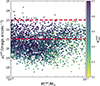 |
Fig. 1. Mean surface brightness (μrcen) as a function of the stellar mass ( |


From the base sample we selected the galaxies with a μrcen value higher than 23 mags arcsec−2, as our LSBG sample, making a total of 26 galaxies. We chose this high threshold in order to analyse an extremely low brightness sample. We also selected a control sample of HSBGs (hereafter the ‘comparison sample’) with galaxies with μrcen values lower than 21 mags arcsec−2 and with stellar masses and  distributions similar to the LSBG sample and a comparable number of galaxies (29). The horizontal dashed red lines in Fig. 1 show the two μrcen thresholds used to determine the samples. In Fig. 2 we show the distributions of μrcen (left),
  (middle), and
  (right) for both samples. Regarding
  and
and  , their distributions are quite similar, with almost the same median value for each sample. This similarity in the
  and
and  distributions was confirmed by a Kolmogorov-Smirnov test, which gave us a p-value greater than 0.8 for both
  and
and  and which heavily implies that the underlying distribution is the same in both cases.
For a better understanding of the samples, we measured different physical properties of the galaxies and their host haloes. In Fig. 3 we show the projected stellar half-mass radius, halo mass (M200), and halo concentration (R200/Rs) distributions. Here, Rs is the scale radius obtained by fitting a Navarro-Frenk-White profile (Navarro et al. 1997) to the dark matter density profile of the halo (we obtain this value from the catalogue by Anbajagane et al. 2022) and the distribution of the dimensionless spin parameter (λ, which we calculate following Bullock et al. 2001). As expected, there is a clear difference in the projected sizes of the galaxies in these samples, with LSBGs showing consistently larger sizes. As a reference, the half-light radius of the Milky Way is 5.75 ± 0.38 kpc (Lian et al. 2024), which is significantly lower than the median value of our LSBGs (13.23 ± 0.9 kpc). We indicate the Milky Way half-light radius with a black arrow in Fig. 3. Despite the fact that the Milky Way and our values are not directly comparable (the Milky Way radius is half light and ours is half stellar mass), both are suitable estimators of galaxy size. On the other hand, there is no significant difference between the masses of the host haloes among the samples. We note that the M200 distributions are marginally, but noticeably, different, with a tendency of LSBGs to reside in slightly more massive haloes. We also note that the R200/Rs values present a slight difference, as the haloes that host LSBGs tend to be less concentrated than haloes hosting galaxies from the comparison sample. According to Pérez-Montaño et al. (2024), there is no difference in concentration related to the surface brightness of the central galaxy, though the samples in that paper are defined in a different way than in this work. The λ parameter shows a more significant difference between our samples, in which LSBGs tend to live in haloes with a high spin. This result is consistent with previous studies (see for instance Kulier et al. 2020; Pérez-Montaño et al. 2022, 2024).
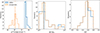 |
Fig. 2. Distributions of the mean surface brightness, μrcen (left panel); stellar mass, |


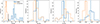 |
Fig. 3. Distribution for the projected stellar half-mass radius ( |

2.2. Satellite galaxies
Since we focus on the characteristics of the satellite system around the central galaxies in both of our samples (LSBGs and comparison), it is important to define which satellites we consider reliable tracers of the structure orbiting those central galaxies. To do this we first removed spurious concentrations of mass that were wrongly identified as subhaloes by SUBFIND and are actually part of the central galaxy (as provided in TNG data). We also applied a mass cut, selecting satellites with a total mass (dark matter, gas, and stars) equivalent to 100 dark matter particles. This threshold corresponds to a total mass equal to 7.5 × 10⁸ M⊙ in TNG100. Finally, we only considered satellites inside the R200 radius of their host haloes. Taking into account these restrictions, we obtained 400 satellites orbiting galaxies in the LSBG sample and 182 associated with galaxies in the comparison sample.
3. Analysis and results
3.1. Analysis of LSBG and comparison samples
For our LSBGs and comparison sample (defined in Sect. 2.1), we wanted to compare the number, distribution, and kinematical properties of the satellites (as defined in Sect. 2.2) orbiting these central galaxies. In Fig. 4 we show the cumulative number of satellites as a function of distance to the central galaxy (in units of R200). The left panel shows the satellite system for each central galaxy in the LSBG sample, with the colour intensity (in blue) indicating the halo mass. The middle panel shows the same statistics for the satellite system around central galaxies in the comparison sample (in oranges). In the right panel we compare the mean number of satellites of both samples. As can be seen, there is a remarkable difference between the mean abundance of the satellites of LSBGs and the satellites of galaxies in the comparison sample, particularly for high-mass haloes, which accounts for a factor of about three times the number of satellites at R200. Thus, this result implies either an original deficiency of satellites associated with HSBGs or otherwise reflects an evolutionary process associated with mergers with the central galaxy.
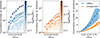 |
Fig. 4. Cumulative number of satellites as a function of the distance to the central galaxy in units of the virial radius (R200) of their host halo. Left panel: LSBG sample (blue shaded). Middle panel: Comparison sample (orange shaded). In both cases, the lines connecting dots correspond to each satellite system of a central galaxy. The colour intensity of each line indicates the mass of the host halo. Right panel: Mean number of satellites of each sample (LSBGs in blue; comparison sample in orange). The bootstrap errors of the median are indicated by the shadowed areas. |
The study presented by Galaz et al. (2011) shows that the distances to the first and fifth nearest neighbours tend to be closer for HSBGs than for LSBGs. Also Rosenbaum et al. (2009), Galaz et al. (2011) found that the number of close neighbours is higher in HSBGs than in LSBGs. Using simulations, Zhu et al. (2023) have found that the distance to the fifth neighbour is larger in LSBGs compared to all galaxies within 10.2 < log(M⋆/M⊙)< 11.6, but closer compared to a sample of galaxies with a stellar, dark matter, and gas mass similar to their LSBG sample. Those results may appear to contradict our results in Fig. 4. However, our analysis focuses on low-mass satellites, and thus it is not comparable with the analysis carried out in these other works. Also, the sample selection for the neighbours in those works are different from our satellite samples, leading to significantly different spatial scales in their studies, with the conclusion that LSBGs tend to form in less dense environments.
In Fig. 5 we show the satellite system velocity dispersion as a function of the stellar mass of central galaxies for the LSBG and comparison samples. Each dot corresponds to the mean velocity dispersion of each satellite system around a central galaxy in each sample. The colour intensity of the dots corresponds to the number of satellites in each system, as indicated by the colour bar. In this analysis, we only consider satellite systems with at least two satellites. Along with a larger number, the satellites of the LSBG sample show a high-velocity dispersion at a given central galaxy stellar mass. Also, as can be seen in this figure, there is an apparent strong correlation for LSBGs. In order to quantify the difference in this relation between the two samples, we applied a linear fit given by
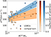 |
Fig. 5. Velocity dispersion (σsat) of the satellite system of each host halo as a function of the stellar mass of the central galaxy. For each sample, the number of satellites is indicated by the shade of the coloured circle: blue circles are for the LSBG sample, and orange circles are for the comparison sample. The solid lines correspond to a linear fit, and the shadowed region indicates the fit error. |
 (2)
(2)
The α and β values derived from the fit are in Table 1. This different behaviour of σsat for the LSBG and comparison samples adds an important difference to the previous result on the number of satellites. We argue that at a given stellar mass of a central galaxy, the detected low velocity dispersion of satellites associated with galaxies in the comparison sample can be explained through a stronger dynamical friction, implying a more efficient merging of satellites onto the central galaxy. We stress the fact that the LSBG and comparison samples have the same distribution of host halo mass, implying that the evolution of the baryonic component of the system of satellites and the stellar concentration of the central galaxies are strongly associated. As mentioned in the introduction, the fate of the remaining satellites may give key clues on the relation between the primary accretion history and its disc formation.

Given the results on the number distribution and velocity dispersion of the satellites in our LSBG and comparison samples, we explored the mass distribution of the stars and the total mass (including stars, gas, and dark matter) for the two samples. We therefore calculated the cumulative mass distributions as a function of distance from the central galaxies in units of R200. The results are shown in Fig. 6, where it can be seen that at distances close to R200, both the total mass and the stellar mass converge to a comparable value. However, in the region nearest the central galaxy and up to ∼1/3R200, the LSBGs have significantly larger cumulative fractions of both stellar and total mass. Thus, our findings reinforce the argument of dynamical friction acting more severely in HSBGs, which may imply a lack of massive satellites at close distances from the central galaxy.
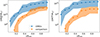 |
Fig. 6. Mean of the cumulative total mass (left panel) and stellar mass (right panel) of satellites as a function of the distance to their central galaxy (in units of R200) for the sample of LSBGs (blue) and comparison sample (orange). The shadowed areas indicate the bootstrap error of the mean. |
3.2. Satellite system properties as a function of the central galaxy  value
value
Another approach for the analysis of the central galaxy surface brightness relation to the local environment is provided in this section, where we determine the characteristics of satellites for central galaxies in the base sample. In this section, we consider  as a continuous value instead of the previously defined LSBG and comparison samples. We split the base sample into two sets of central galaxies according to their stellar mass – in low-mass
  and in high-mass
  – in order to have the same number of central galaxies, i.e. 1555, in each set. Then, we selected the corresponding satellites following the same procedure detailed in Sect. 2.2. We obtained a total of 6212 satellites in the low-mass subsample and 20 040 satellites in the high-mass subsample.
Using the previously described set of satellites, Fig. 7 shows the median number of satellites as a function of  for the base sample (grey line), the high-mass sample (pink line), and the low-mass (indigo line) sample. We utilise the same colour code used in this figure for the remaining figures. In general, the number of satellites has a significant host-surface-brightness dependence, where galaxies in both the bright and faint end of the μrcen distribution host a larger number of satellites in comparison to galaxies in the intermediate μrcen range. At the same time, this signal has a stellar-mass dependence, being more evident in the range of massive galaxies (pink line). However, we note the similarity between the relative increase in the number of satellites for the different central galaxy mass ranges. Overall, these results are consistent with Fig. 4.
Finally, to further explore the dynamics of satellites and take into account the results of Fig. 5, we calculated the ratio of velocity modulus normal to the radial direction to the total velocity ( ) for the satellite system as a function of
  , which is shown in the left panel of Fig. 8 for the high-mass (pink), low-mass (indigo), and base (grey) samples. As can be seen, there is an increasing trend for non-radial motions towards high values of
  . This is stronger for the low-mass central galaxies, presumably motivated by the excess of angular momentum of the dark matter haloes of LSBGs with respect to the comparison sample (see the rightmost panel in Fig. 3). Studies such as Di Cintio et al. (2019), Wright et al. (2025), Wu et al. (2025) present evidence that LSBGs have undergone mergers in which the secondary orbit were, in general, co-planar with respect to the primary gas disc. For HSBGs, however, this is not the case. The results shown here could be a sign of this behaviour.
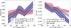 |
Fig. 8. Magnitude of the tangential velocity normalised to the magnitude of the total velocity ( |


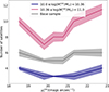 |
Fig. 7. Median number of satellites as a function of the surface brightness (μrcen) for all central galaxies in the analysed mass range. The galaxies are split by stellar mass in low-mass ( |


We also computed the scalar product between the normalised orbital angular momentum of the system of satellites ( ) and the normalised angular momentum of the stellar component of the central galaxy (
 ) as a function of surface brightness,
  . These results are in the right panel of Fig. 8, where a value of
  indicates that the satellite system and the angular momentum of the central galaxy are co-rotating, while a negative value indicates that the galaxy and its satellites are counter-rotating. As can be seen in this figure, there is a strong anti-correlation of the alignment of the disc of the central galaxy and the orbit of the satellites with
  , which is more evident for the low-mass sample (indigo line). This means that the amount of orbital angular momentum in counter-rotating satellites with respect to the angular momentum of the disc decreases with the surface brightness of the central galaxy. We argue that this is an expected result in a scenario where the preferred accretion of co-rotating satellites onto galaxies evolving into LSBGs leaves their population of remaining satellites preferentially in counter-rotation. This last result is in agreement with the observational evidence that shows that the specific angular momentum of LSBGs tends to be higher when compared to that computed in HSGBs (Pérez-Montaño & Cervantes Sodi 2019; Jadhav Y & Banerjee 2019). This behaviour is also present in simulations (Salinas & Galaz 2021; Pérez-Montaño et al. 2022; Zhu et al. 2023; Pallero et al. 2025).
4. Discussion
The abundance of satellites and their dynamics can be used as a probe that could be crucial for understanding the emergence of LSBGs. In this sense, this work can serve as a theoretical motivation for observational studies of these systems. This gains special interest when considering the upcoming data from the Legacy Survey of Space and Time (LSST; Ivezić et al. 2019), which will allow the study of currently undiscovered low-brightness regions. We argue that not only baryonic physics but also gravity models may be tested in detail in future analyses of LSBGs studies. In the literature, there are theoretical predictions about the effect of different gravity models on the formation of LSBGs (for instance see Müller et al. 2019a; Nagesh et al. 2024, which analyses the effect of MOND models). The remarkable differences in the spatial distribution and dynamics of satellites associated with either the LSBG sample or the comparison sample in a Λ cold dark matter scenario give hints that these systems can provide relevant tests of these fundamental aspects.
Among the main results of our analysis is the higher cumulative number of satellites for the LSBG sample with respect to the comparison sample of similar stellar mass and morphology (Fig. 4). We obtained an increasing difference in the abundance of satellites, which reaches a factor of about three at R200. The possibility that this significant difference comes from a primordial origin or that it comes as a result of evolution was further explored. In particular, the cumulative distribution in stellar and total mass was analysed for the LSBG and comparison samples (Fig. 6). We found that at distances approaching R200, both the total and stellar mass are similar in the two cases. Nevertheless, the mass of the satellite systems (stellar and total) at distances closer than ∼1/3 R200 is significantly larger for the LSBG sample than in the comparison sample. We argue that this points towards a dynamical evolution origin driven by a strong dynamical friction in systems evolving into HSBGs via mergers, which would cause a lack of massive satellites close to the central galaxies.
Regarding the dynamics of the satellite system, we find that their mean velocity dispersion as a function of the central stellar mass is highly correlated for the LSBGs. On the contrary, for satellites associated with the comparison sample, the correlation is significantly poorer (Fig. 5). Since our LSBG and comparison samples have a very similar halo mass, a different evolution of the system of satellites associated with the stellar density of the central galaxies must have been in action. This is further supported by the lack of co-rotating satellites in LSBGs with respect to the comparison sample as shown in Fig. 8. We claim that this is a clear hint of the accretion of co-rotating satellites by central galaxies in the process of a LSBG-type evolution. Accretions in co-rotation are expected to be less disruptive than for satellites counter-rotating or in radial trajectories. In fact, several recent studies have indicated that the acquisition of angular momentum from accreted material, co-rotating or otherwise aligned with the disc angular momentum, contributes to the formation of extended diffuse discs by enhancing the net spin of the central system and limiting disc heating (Di Cintio et al. 2019; Wright et al. 2025; Wu et al. 2025). Such aligned infall channels allow galaxies to maintain lower central stellar densities and more extended stellar distributions and are consistent with the structural properties observed in LSBGs. This orbital behaviour would be more frequently associated with the merger of satellites of the comparison sample, which would conserve the isotropic distribution of rotating and counter-rotating satellites, as is observed in our analysis.
Our analysis of the satellite systems of galaxies with a range of surface brightnesses sheds light on the phenomena that take place in the formation of the structures with a low surface brightness. The distribution and dynamics of satellites could provide evidence of the accretion history of central galaxies. The lack of previous hydrodynamical studies concerning the analysis of the satellite systems associated with LSBGs is related to the fact that the required resolution in hydrodynamical simulations has only been achieved in recent years with the advent of large hydrodynamical simulations such as IllustrisTNG (Pillepich et al. 2018b; Weinberger et al. 2017) or Eagle (Crain et al. 2015; Schaye et al. 2015). For instance, some of the studies on LSBGs that take advantage of these state-of-art simulations are Pérez-Montaño et al. (2022, 2024), Pallero et al. (2025). In particular, Zhu et al. (2023) state that the population of LSBGs accounts only for 6% of the galaxies in the mass range given by 1010.2 ≤ M⋆/M⊙ ≤ 1011.6, challenging their observational detection. Despite these difficulties, some observational studies have been able to characterise the properties and environment of LSGBs (for instance Pérez-Montaño & Cervantes Sodi 2019). The predictions presented in this work could serve as inspiration for future observational analysis of LSBGs and their satellite systems, especially when used in combination with the large upcoming surveys that will reach deeper magnitude limits than the available observational data, such as the LSST or Euclid (Laureijs et al. 2011).
Acknowledgments
The authors would like to thanks to the anonymous referee for their invaluable comments and suggestions, which help to improve this work greatly. SR and YY acknowledge financial support from FONCYT through the PICT 2019-1600 grant. JAB is grateful for partial financial support from the NSF-CAREER-1945310 and NSF-AST-2107993 grants. SP acknowledges partial support from ANPCyT (Argentina) through grant PICT 2020-00582. GG acknowledges the support of the ANID BASAL project CATA FB210003, as well as the support of the French-Chilean Laboratory for Astronomy (FCLA).
References
- Anbajagane, D., Evrard, A. E., & Farahi, A. 2022, MNRAS, 509, 3441 [Google Scholar]
- Benavides, J. A., Sales, L. V., Abadi, M. G., et al. 2023, MNRAS, 522, 1033 [NASA ADS] [CrossRef] [Google Scholar]
- Benavides, J. A., Sales, L. V., Abadi, M. G., et al. 2024, ApJ, 977, 169 [NASA ADS] [CrossRef] [Google Scholar]
- Bullock, J. S., Dekel, A., Kolatt, T. S., et al. 2001, ApJ, 555, 240 [NASA ADS] [CrossRef] [Google Scholar]
- Chan, T. K., Kereš, D., Wetzel, A., et al. 2018, MNRAS, 478, 906 [NASA ADS] [CrossRef] [Google Scholar]
- Crain, R. A., Schaye, J., Bower, R. G., et al. 2015, MNRAS, 450, 1937 [NASA ADS] [CrossRef] [Google Scholar]
- Davis, M., Efstathiou, G., Frenk, C. S., & White, S. D. M. 1985, ApJ, 292, 371 [Google Scholar]
- de Blok, W. J. G., & McGaugh, S. S. 1997, MNRAS, 290, 533 [NASA ADS] [CrossRef] [Google Scholar]
- Di Cintio, A., Brook, C. B., Macciò, A. V., Dutton, A. A., & Cardona-Barrero, S. 2019, MNRAS, 486, 2535 [NASA ADS] [CrossRef] [Google Scholar]
- Dolag, K., Borgani, S., Murante, G., & Springel, V. 2009, MNRAS, 399, 497 [Google Scholar]
- Dubois, Y., Pichon, C., Welker, C., et al. 2014, MNRAS, 444, 1453 [Google Scholar]
- Galaz, G., Herrera-Camus, R., Garcia-Lambas, D., & Padilla, N. 2011, ApJ, 728, 74 [NASA ADS] [CrossRef] [Google Scholar]
- Huchra, J. P., & Geller, M. J. 1982, ApJ, 257, 423 [NASA ADS] [CrossRef] [Google Scholar]
- Ivezić, Ž., Kahn, S. M., Tyson, J. A., et al. 2019, ApJ, 873, 111 [Google Scholar]
- Jadhav Y, V., & Banerjee, A. 2019, MNRAS, 488, 547 [NASA ADS] [CrossRef] [Google Scholar]
- Kim, J.-H., & Lee, J. 2013, MNRAS, 432, 1701 [Google Scholar]
- Kulier, A., Galaz, G., Padilla, N. D., & Trayford, J. W. 2020, MNRAS, 496, 3996 [NASA ADS] [CrossRef] [Google Scholar]
- Kuzio de Naray, R., McGaugh, S. S., & de Blok, W. J. G. 2004, MNRAS, 355, 887 [Google Scholar]
- Laureijs, R., Amiaux, J., Arduini, S., et al. 2011, ArXiv e-prints [arXiv:1110.3193] [Google Scholar]
- Lelli, F., Fraternali, F., & Sancisi, R. 2010, A&A, 516, A11 [NASA ADS] [CrossRef] [EDP Sciences] [Google Scholar]
- Lian, J., Zasowski, G., Chen, B., et al. 2024, Nat. Astron., 8, 1302 [Google Scholar]
- Marinacci, F., Vogelsberger, M., Pakmor, R., et al. 2018, MNRAS, 480, 5113 [NASA ADS] [Google Scholar]
- Martin, G., Kaviraj, S., Laigle, C., et al. 2019, MNRAS, 485, 796 [NASA ADS] [CrossRef] [Google Scholar]
- Mo, H. J., McGaugh, S. S., & Bothun, G. D. 1994, MNRAS, 267, 129 [NASA ADS] [CrossRef] [Google Scholar]
- Müller, O., Famaey, B., & Zhao, H. 2019a, A&A, 623, A36 [Google Scholar]
- Müller, O., Rich, R. M., Román, J., et al. 2019b, A&A, 624, L6 [Google Scholar]
- Nagesh, S. T., Freundlich, J., Famaey, B., et al. 2024, A&A, 690, A149 [NASA ADS] [CrossRef] [EDP Sciences] [Google Scholar]
- Naiman, J. P., Pillepich, A., Springel, V., et al. 2018, MNRAS, 477, 1206 [Google Scholar]
- Navarro, J. F., Frenk, C. S., & White, S. D. M. 1997, ApJ, 490, 493 [Google Scholar]
- Nelson, D., Pillepich, A., Springel, V., et al. 2018, MNRAS, 475, 624 [Google Scholar]
- Nelson, D., Springel, V., Pillepich, A., et al. 2019, Comput. Astrophys. Cosmol., 6, 2 [Google Scholar]
- Pallero, D., Galaz, G., Tissera, P. B., et al. 2025, A&A, 699, A376 [NASA ADS] [CrossRef] [EDP Sciences] [Google Scholar]
- Papastergis, E., Adams, E. A. K., & Romanowsky, A. J. 2017, A&A, 601, L10 [NASA ADS] [CrossRef] [EDP Sciences] [Google Scholar]
- Pérez-Montaño, L. E., & Cervantes Sodi, B. 2019, MNRAS, 490, 3772 [CrossRef] [Google Scholar]
- Pérez-Montaño, L. E., Rodriguez-Gomez, V., Cervantes Sodi, B., et al. 2022, MNRAS, 514, 5840 [CrossRef] [Google Scholar]
- Pérez-Montaño, L. E., Cervantes Sodi, B., Rodriguez-Gomez, V., Zhu, Q., & Ogiya, G. 2024, MNRAS, 533, 93 [Google Scholar]
- Pillepich, A., Nelson, D., Hernquist, L., et al. 2018a, MNRAS, 475, 648 [Google Scholar]
- Pillepich, A., Springel, V., Nelson, D., et al. 2018b, MNRAS, 473, 4077 [Google Scholar]
- Planck Collaboration XIII. 2016, A&A, 594, A13 [NASA ADS] [CrossRef] [EDP Sciences] [Google Scholar]
- Press, W. H., & Davis, M. 1982, ApJ, 259, 449 [Google Scholar]
- Rodriguez, F., Montero-Dorta, A. D., Angulo, R. E., Artale, M. C., & Merchán, M. 2021, MNRAS, 505, 3192 [NASA ADS] [CrossRef] [Google Scholar]
- Rong, Y., Zhu, K., Johnston, E. J., et al. 2020, ApJ, 899, L12 [CrossRef] [Google Scholar]
- Rong, Y., Hu, H., He, M., et al. 2024, ArXiv e-prints [arXiv:2404.00555] [Google Scholar]
- Rosenbaum, S. D., Krusch, E., Bomans, D. J., & Dettmar, R.-J. 2009, A&A, 504, 807 [NASA ADS] [CrossRef] [EDP Sciences] [Google Scholar]
- Saburova, A. S., Chilingarian, I. V., Kasparova, A. V., et al. 2021, MNRAS, 503, 830 [NASA ADS] [CrossRef] [Google Scholar]
- Sales, L. V., Navarro, J. F., Schaye, J., et al. 2010, MNRAS, 409, 1541 [Google Scholar]
- Sales, L. V., Navarro, J. F., Theuns, T., et al. 2012, MNRAS, 423, 1544 [Google Scholar]
- Salinas, V. H., & Galaz, G. 2021, ApJ, 915, 125 [NASA ADS] [CrossRef] [Google Scholar]
- Schaye, J., Crain, R. A., Bower, R. G., et al. 2015, MNRAS, 446, 521 [Google Scholar]
- Schombert, J., & McGaugh, S. 2021, AJ, 161, 91 [Google Scholar]
- Springel, V., White, S. D. M., Tormen, G., & Kauffmann, G. 2001, MNRAS, 328, 726 [Google Scholar]
- Springel, V., Pakmor, R., Pillepich, A., et al. 2018, MNRAS, 475, 676 [Google Scholar]
- Tang, L. 2024, MNRAS, 530, 812 [Google Scholar]
- Wang, L., Dutton, A. A., Stinson, G. S., et al. 2015, MNRAS, 454, 83 [NASA ADS] [CrossRef] [Google Scholar]
- Weinberger, R., Springel, V., Hernquist, L., et al. 2017, MNRAS, 465, 3291 [Google Scholar]
- Wright, A. C., Tremmel, M., Brooks, A. M., et al. 2021, MNRAS, 502, 5370 [NASA ADS] [CrossRef] [Google Scholar]
- Wright, A. C., Brooks, A. M., Tremmel, M., et al. 2025, ArXiv e-prints [arXiv:2507.21231] [Google Scholar]
- Wu, X., Zhu, L., Chang, J., Zeng, G., & Lei, Y. 2025, A&A, 699, A374 [NASA ADS] [CrossRef] [EDP Sciences] [Google Scholar]
- Wyder, T. K., Martin, D. C., Barlow, T. A., et al. 2009, ApJ, 696, 1834 [NASA ADS] [CrossRef] [Google Scholar]
- York, D. G., Adelman, J., Anderson, J. E., Jr., et al. 2000, AJ, 120, 1579 [NASA ADS] [CrossRef] [Google Scholar]
- Zhu, Q., Pérez-Montaño, L. E., Rodriguez-Gomez, V., et al. 2023, MNRAS, 523, 3991 [NASA ADS] [CrossRef] [Google Scholar]
We define the supra index cen as an indication that the quantity corresponds to central galaxies, while the supra index sat indicates that a quantity was measured for satellites.
All Tables
All Figures
|
Fig. 1. Mean surface brightness (μrcen) as a function of the stellar mass ( |
| In the text | |
|
Fig. 2. Distributions of the mean surface brightness, μrcen (left panel); stellar mass, |
| In the text | |
|
Fig. 3. Distribution for the projected stellar half-mass radius ( |
| In the text | |
|
Fig. 4. Cumulative number of satellites as a function of the distance to the central galaxy in units of the virial radius (R200) of their host halo. Left panel: LSBG sample (blue shaded). Middle panel: Comparison sample (orange shaded). In both cases, the lines connecting dots correspond to each satellite system of a central galaxy. The colour intensity of each line indicates the mass of the host halo. Right panel: Mean number of satellites of each sample (LSBGs in blue; comparison sample in orange). The bootstrap errors of the median are indicated by the shadowed areas. |
| In the text | |
|
Fig. 5. Velocity dispersion (σsat) of the satellite system of each host halo as a function of the stellar mass of the central galaxy. For each sample, the number of satellites is indicated by the shade of the coloured circle: blue circles are for the LSBG sample, and orange circles are for the comparison sample. The solid lines correspond to a linear fit, and the shadowed region indicates the fit error. |
| In the text | |
|
Fig. 6. Mean of the cumulative total mass (left panel) and stellar mass (right panel) of satellites as a function of the distance to their central galaxy (in units of R200) for the sample of LSBGs (blue) and comparison sample (orange). The shadowed areas indicate the bootstrap error of the mean. |
| In the text | |
|
Fig. 8. Magnitude of the tangential velocity normalised to the magnitude of the total velocity ( |
| In the text | |
|
Fig. 7. Median number of satellites as a function of the surface brightness (μrcen) for all central galaxies in the analysed mass range. The galaxies are split by stellar mass in low-mass ( |
| In the text | |
Current usage metrics show cumulative count of Article Views (full-text article views including HTML views, PDF and ePub downloads, according to the available data) and Abstracts Views on Vision4Press platform.
Data correspond to usage on the plateform after 2015. The current usage metrics is available 48-96 hours after online publication and is updated daily on week days.
Initial download of the metrics may take a while.