| Issue |
A&A
Volume 707, March 2026
|
|
|---|---|---|
| Article Number | A311 | |
| Number of page(s) | 15 | |
| Section | Galactic structure, stellar clusters and populations | |
| DOI | https://doi.org/10.1051/0004-6361/202557469 | |
| Published online | 24 March 2026 | |
Primordial segregation in globular clusters: The degree of mass segregation as determined through dynamical models
1
Department of Mathematics and Physics, University of Campania Luigi Vanvitelli,
viale Lincoln 5,
81100
Caserta,
Italy
2
INAF – Osservatorio Astronomico d’Abruzzo,
Via Mentore Maggini snc,
64100
Teramo,
Italy
3
INFN – sezione di Roma,
Piazzale Aldo Moro 2,
00185
Rome,
Italy
4
Department of Physics, University of Rome La Sapienza,
Piazzale Aldo Moro 2,
00185
Rome,
Italy
5
INFN Sezione di Napoli,
Via Cintia snc,
80126
Napoli,
Italy
★ Corresponding author: This email address is being protected from spambots. You need JavaScript enabled to view it.
; This email address is being protected from spambots. You need JavaScript enabled to view it.
Received:
29
September
2025
Accepted:
4
February
2026
Abstract
Context. Globular clusters (GCs) are dense stellar systems whose dynamics, which are driven by two-body relaxation, exhibit mass-based processes such as mass segregation and energy equipartition. However, a satisfactory description and quantification of mass segregation is still lacking.
Aims. We characterize the degree of mass segregation through a multi-mass dynamical model that also predicts energy equipartition. Our work focuses on the generation of initial conditions for primordially segregated clusters. We show that these conditions are suitable for N-body simulations of GCs and their multiple populations.
Methods. We quantified the degree of mass segregation by looking at the relation between half-mass radius and stellar mass. We describe how the model inputs change the shape of this function. Furthermore, we developed a customized version of the MCLUSTER code to generate a stellar system based on our dynamical model.
Results. For any degree of mass segregation, the half-mass radius exhibits a linearly decreasing relationship with the stellar mass. Our analysis reveals that the main parameter responsible for the degree of segregation is Φ0, which represents the strength of the gravitational potential. It is also related to the slope β of the linear approximation. Conversely, the mass function only plays a minor role, where steeper slopes and larger mass ranges result in a slight increase in the degree of segregation. Concerning the generation of stars, our approach successfully provides stellar physical properties, such as density and mean square velocity, and reproduces well the corresponding theoretical profiles. We explore possible realistic initial conditions, such as a Kroupa initial mass function with Φ0 = 0.01 and 0.1 M⊙−1, which correspond to a negligible segregation and a highly segregated reference case, respectively. In the context of a two-generation scenario, we can model first-generation stars that exhibit a degree of primordial segregation resulting from violent relaxation. Furthermore, we explore variations in the time elapsed between the formation of the first and the second stellar generations; we consider time intervals of up to 100 Myr, which is a range that is consistent with the asymptotic giant branch self-pollution scenario.
Conclusions. This work further proves the ability of our multi-mass dynamical models to predict mass-based processes, with a focus on mass segregation. This model offers the possibility to set up primordially segregated clusters in a consistent way, and can help us to constrain the poorly understood early phases of GCs and the evolution of their multiple populations.
Key words: stars: kinematics and dynamics / globular clusters: general
© The Authors 2026
 Open Access article, published by EDP Sciences, under the terms of the Creative Commons Attribution License (https://creativecommons.org/licenses/by/4.0), which permits unrestricted use, distribution, and reproduction in any medium, provided the original work is properly cited.
This article is published in open access under the Subscribe to Open model. This email address is being protected from spambots. You need JavaScript enabled to view it. to support open access publication.
1 Introduction
Among stellar systems, globular clusters (GCs) are the only known collisional systems where two-body relaxation shapes their structure, as well as their spatial and kinematic features, for most of their life (Spitzer 1987; Binney & Tremaine 2008). It was commonly believed that GCs were made of a single stellar population, with the relaxation process bringing stars toward kinetic energy equipartition and mass segregation on a few relaxation timescales, trelax. Equipartition tends to produce slower high-mass stars and faster low-mass stars. The energy exchange due to encounters leads to segregation, that is, the sinking of bright and massive stars toward central regions, while low-mass stars are more spread across the cluster and are dominant close to the edge. GCs also suffer the loss of stars due to the Galactic tidal field, typically called evaporation (Hénon 1961; Henon 1969; Spitzer 1987; Gnedin & Ostriker 1997). This effect acts according to the environment, which is primarily determined by the Galactic potential and the orbital properties of the cluster, as well as internal dynamics. It is influenced by equipartition and segregation that favor the loss of the fast low-mass stars. Thus, evaporation probably has its own timescale, tev. Furthermore, GCs are at virial equilibrium, which means they are dynamically stable. Virialization follows the crossing timescale, tcross, and determines the dynamical equilibrium of the system (Lynden-Bell 1967; Binney & Tremaine 2008). When evaporation removes stars, the system reacts to maintain virial equilibrium and allows the relaxation process, which acts on longer timescales, to shape the properties of the system. The phenomena mentioned constitute the equipartition-segregation-evaporation-virialization (ESEV) puzzle (Merafina 2018), which summarizes the dynamical processes of GCs, whose interplay still lacks a definitive description. A schematic view of such a puzzle is given in Fig. 1, where we associate an individual timescale to each process. The circularity of the diagram shows the entire evolution as a continuous path toward complete relaxation.
The evidence for the existence of multiple stellar populations (MPs) opens a variety of new challenges, mainly regarding their formation and early evolutionary phases, which further complicate the overall picture. The formation of MPs is widely debated: several scenarios have been proposed, yet a full explanation for the observed properties remains elusive (Bastian & Lardo 2018).
The variety of the processes involves several fields of astrophysics. Among them, an important role is played by the stellar formation processes in a poorly known early galactic environment. According to most of the scenarios proposed for MP formation, the first generation (FG) of stars is produced from a gas with a nearly primordial composition and, subsequently, a second generation (SG) is produced from the material lost by FG stars that is eventually diluted with a pristine gas (Gratton et al. 2019). When SG stars form, the cluster environment is dominated by the FG gravitational field. As a consequence, SG stars preferentially form in the innermost region (D’Ercole et al. 2008; Calura et al. 2019). However, the initial, or primordial, density profiles of both FG and SG stars are unknown. Extant dynamical evolution studies often adopt a density profile from the King (1966) model, which is a dynamical model obtained by assuming that all stars have the same mass. Nevertheless, a mass distribution is assigned according to an initial mass function (IMF). Moreover, current state-of-the-art MP simulations use the same King model to generate both FG and SG stars (Vesperini et al. 2013, 2018, 2021). This scheme does not consider the occurrence of a primordial mass segregation.
As already mentioned, mass segregation was commonly believed to occur only during the long-term dynamical evolution of GCs due to relaxation. However, a variety of works have shown that GCs arise from their violent relaxation phase as already segregated in mass, with a degree of internal rotation and anisotropy (Livernois et al. 2021, and refs therein). Violent relaxation consists of an early dynamical phase that occurs after the formation of stars and brings the cluster to virial equilibrium (Lynden-Bell 1967), producing the final monolithic structure. The properties that clusters show after such a phase can play an important role in shaping their long-term evolution. In particular, during violent relaxation, sub-clumps are formed on a shorter timescale (Goodwin & Whitworth 2004) and are characterized by a higher spatial concentration of massive stars (McMillan et al. 2007; Allison et al. 2009). This segregation of masses seems to occur under different initial conditions (ICs; Domínguez et al. 2017). In addition, the presence of the Galactic tidal field alters the kinematic fingerprint of the clusters, such as internal rotation and anisotropy in velocities, during this early phase (Vesperini et al. 2014).
Typical N-body simulations that account for a mass distribution do not consider primordial segregation. The most widespread choice is to generate stellar masses according to a power-law IMF (often taken from Kroupa 2001, eventually with variations of the slopes and mass extremes) and use a King (1966) distribution function (DF) to assign positions and velocities; as a consequence, no link is made to the mass of the stars (see, for example, ICs by Vesperini & Heggie 1997; Joshi et al. 2001; Baumgardt & Makino 2003; Trenti & van der Marel 2013; Giersz et al. 2015; Leigh et al. 2015; Wang et al. 2016; Sollima & Baumgardt 2017; Pavlík & Vesperini 2021; Livernois et al. 2022, 2024). Some works in the literature considered the role of primordial mass segregation in the dynamical evolution of GCs (Vesperini et al. 2009; Haghi et al. 2014). Usually, empirical approaches are employed to establish primordial segregation, such as ordering criteria or adopting a specific shape of the gravitational potential (Šubr et al. 2008; Baumgardt et al. 2008). Alternatively, the cluster is left to evolve for a limited time until it develops segregation through relaxation (Vesperini et al. 2009). A few attempts have been made to use multi-mass dynamical models to set primordial segregation for MPs (such as the work by Sollima 2021, which used the Gunn & Griffin (1979) model), as inputs for Monte Carlo simulations. Nonetheless, a rigorous description and quantification of mass segregation is still lacking.
In this work, we show that our multi-mass King-like dynamical model (Teodori et al. 2024) is able to predict self-consistently the degree of mass segregation, according to the inputs of the model. It works not only for primordial segregation but also for current segregation. We also provide an empirical counterpart that helps in the evaluation of the degree of mass segregation. In addition, our model provides a useful tool for generating primordially segregated ICs, and offers a theoretically based approach with respect to empirical and existing methods. This can be applied to the study of MPs’ dynamical evolution through N-body simulations, from the perspective of accounting for a primordial segregation degree in the FG that results from violent relaxation. This aspect, coupled with the early mass loss triggered by stellar evolution, may alter the mass function of the FG from the very beginning of the relaxation process, and may favor the evaporation of low-mass stars that would populate the Galactic halo.
 |
Fig. 1 ESEV puzzle schematic representation. |
2 Methods
The central point of our work lies in the prediction of mass segregation by means of a multi-mass King-like dynamical model. A measure of the degree of segregation is shown in terms of model parameters, as well as a linear relation between the half-mass radius and the stellar mass. We used the dynamical model to generate GCs stars, and linked the distribution of positions and velocities with mass. This provides a theoretical tool for investigating the role of a primordial segregation degree through N-body simulations.
2.1 The segregation degree
The main observable that we used to look at mass segregation was the dependence of the half-mass radius on the stellar mass, rh(m). Its shape is related to the degree of mass segregation, as we discuss in the paper. This quantity is predicted by the dynamical model and can be approximated with a linear relation.
2.1.1 Multi-mass dynamical model
In this work, we used an original multi-mass dynamical model based on a King-like DF that proved capable of predicting and quantifying the mass-based processes that occur in GCs, such as energy equipartition (Teodori et al. 2024). It also provided a good fit for surface brightness profiles for GCs. As shown later in this paper, we found that it can also successfully describe mass segregation.
The King (1965, 1966) model was obtained by an approximate solution of the Fokker-Planck equation as resulting from the Boltzmann collisional equation for gravitational encounters (Chandrasekhar 1943; Spitzer & Härm 1958; Chandrasekhar 1960; Binney & Tremaine 2008). While the King DF accounts for all equal masses, our model shows a similar derivation that accounts for the presence of a mass distribution for stars (as first done by Da Costa & Freeman 1976). More details can be found in Teodori et al. (2024, Appendix A). The model is defined by its DF, which characterizes the distribution of stars in mass, m, position, r, and velocity, v. Its expression is
![Mathematical equation: $g(r,v,m) = k(m){{\rm{e}}^{ - m\left[ {\varphi (r) - {\varphi _0}} \right]/\left( {{k_{\rm{B}}}\theta } \right)}}\left[ {{{\rm{e}}^{ - \varepsilon (v,m)/\left( {{k_{\rm{B}}}\theta } \right)}} - {{\rm{e}}^{ - {\varepsilon _{\rm{c}}}(r,m)/\left( {{k_{\rm{B}}}\theta } \right)}}} \right],$](/articles/aa/full_html/2026/03/aa57469-25/aa57469-25-eq2.png) (1)
(1)
where φ is the gravitational potential (with φ0 its central value), ε = mv2/2 is the kinetic energy, and  is the cut-off kinetic energy, with ve(r) being the escape velocity that depends on the radial coordinate, r. The factor k(m) is related to the mass function (see Teodori et al. 2024, Appendix A), while θ is the thermodynamic temperature (Merafina 2017, 2018, 2019) and kB is the Boltzmann constant.
The DF in Eq. (1) defines the radial profile of mass density, ρ(r), by integration over velocities and masses. This quantity is used to obtain the gravitational potential by solving the Poisson equation in dimensionless units, and thus determining the equilibrium configuration.
To obtain the half-mass radius, rh(m), we need the cumulative mass profile, M(r, m), of stars with a mass, m (i.e., belonging to a mass bin) that can be computed by the density profile ρ(r, m). The latter quantity is obtained by integration over the velocities of Eq. (1). The condition M(rh, m) = Mtot(m)/2 defines rh(m), that is, the radius where we reach half the total mass of stars with mass, m. All quantities are provided by the model in dimensionless units so that we directly obtain rh(m)/rt, where rt is the tidal radius. The shape of this function is connected to the degree of mass segregation. In a segregated configuration, massive stars are more concentrated in the center. Thus, the cumulative mass profile for such stars is steeper and the corresponding half-mass radius is smaller. The opposite holds true for low-mass stars. As a consequence, any degree of segregation should produce a trend for rh(m)/rt that decreases with increasing mass. The prediction for rh(m)/rt depends on the input parameters of the model. The most important parameter is the gravitational potential well, through the Φ0 = (φR − φ0)/(kBθ) parameter, where φR is the gravitational potential at the edge. The value of Φ0 determines the IC needed to solve the dimensionless Poisson equation (Teodori et al. 2024). Then we have the shape of the mass function that is assumed to be a single power law with slope α, which is valid in the range [mmin, mmax], or a double power law, with α1 valid for mmin ≤ m < 0.5 M⊙ and α2 valid for 0.5 M⊙ ≤ m ≤ mmax. All such parameters identify the equilibrium configuration and thus can contribute to the degree of mass segregation, as we show in Sect. 3.1.
Note that the model and discussion above is meant for GCs that are characterized by a density profile that monotonically decreases with the radial distance, which is a consequence of the DF shape. This is also valid for the density profile of each mass, m. Thus, mass segregation is defined in terms of central spatial concentration. On the contrary, other stellar systems such as open clusters (OCs) are morphologically different and the relation between a higher radial concentration of massive stars and a higher segregation is not necessarily valid, in particular for those showing a fractal distribution. Mass segregation in OCs is typically measured with the local surface density ratio (Maschberger & Clarke 2011; Parker & Goodwin 2015), which is the surface density of the most massive stars with respect to all stars in local regions and does not necessarily require a radial profile. According to Coenda et al. (2025), ≈80% of OCs are segregated and among these, 76% of single OCs show a radial profile, while OCs in pairs and groups have a smaller fraction. This suggests that our approach could be applied to single OCs that show a radial profile, but further investigation into their dynamical phase is needed to verify whether such objects can be described by our DF. This goes beyond the scope of this work, which is dedicated to the degree of mass segregation in GCs.
Furthermore, we clarify that the Galactic tidal field experienced by GCs during their evolution alters their properties. Our King-like DF accounts for tidal effects through the cut-off energy. Thus, stars that experience gravitational encounters and get a kinetic energy that overcomes the cut-off value are not considered. During evolution, the effect of segregation and the tidal field lead to the preferential evaporation of the low-mass stars, which are also typically more numerous. This implies that, as evolution proceeds, the mass function is depleted in the low-mass regime by these processes, in addition to stellar evolution that mainly affects the high-mass tail. Thus, to describe GCs at different phases with our model, we need to consider variations in the mass function input parameters, namely the slope and the mass range.
2.1.2 Linear relation
We introduce an empirical law to quantify the mass segregation degree; this is a linear relation between rh/rt and the mass m, namely
 (2)
(2)
The β parameter estimates the slope of rh(m) at first order and thus provides an empirical measure of the segregation degree, which is of practical use due to the simplicity of the adopted function. The linear approximation also shows how the prediction of the dynamical model changes for different inputs.
Our empirical estimator of mass segregation β and the rh(m) relation predicted by the model can only be qualitatively compared with other methods in the literature. Observationally, there are several ways to estimate mass segregation. Concerning primordial mass segregation, one possibility is through the local variation of the slope of a single power-law mass function α(r), as done for Magellanic Cloud clusters (Gouliermis et al. 2004; Kerber & Santiago 2006) and OCs (Hasan & Hasan 2011; Pang et al. 2013). In the core, the mass function slope is higher (α is negative, thus a higher value means a flatter mass function) due to the higher concentration of massive stars with respect to outer regions, where the slope value is lower (steeper mass function). Furthermore, in OCs mass segregation is observationally evaluated through the local density ratio ΣLDR (Maschberger & Clarke 2011; Coenda et al. 2025), which is the ratio of average spatial lengths between classes of stars Λmsr and lMST (Allison et al. 2009; Beccari et al. 2012; Dib et al. 2018), also used for dense molecular clouds (Dib & Henning 2019). We refer the reader to the work by Parker & Goodwin (2015) for a summary of the estimators mentioned. It has been pointed out that such quantities suffer biases and selection effects, such as incompleteness, which is especially important in cluster cores due to crowding effects that are not properly corrected (Ascenso et al. 2009). Concerning GCs, typical observational evidence for the current mass segregation is again seen in terms of α(r) (Zhang et al. 2015; Beccari et al. 2015; Baumgardt & Sollima 2017) and the area A+ between the cumulative radial distribution of massive objects like blue straggler stars and reference stars (Dalessandro et al. 2015; Ferraro et al. 2012, 2018).
With the exception of α(r), all the other parameters quantify the relative spatial distribution between massive stars and other stars. Thus, stars are first grouped according to their mass, and then their spatial extension is compared. This is qualitatively similar to how rh(m) is obtained, but in our dynamical model each value is uniquely associated to the corresponding mass and does not rely on other mass classes to be defined. The radial distribution is provided by the cumulative mass profile, M(r, m). Furthermore, in our approach, the value of β only approximates the mass segregation degree at the first order, which is represented by rh(m) itself. Additionally, the half-mass radius relation with stellar mass slightly changes the definition of mass segregation. Here, more massive stars show a steeper cumulative mass distribution, and yield a lower half-mass radius with respect to stars with a lower mass. This is applicable to systems that have a radial profile, as discussed in Sect. 3.1, thus, primarily GCs.
Regarding α(r), an estimate of the segregation degree requires us to obtain a quantity that uniquely defines the shape of this function and quantifies segregation. This parameter can potentially be related to our β, but this requires devoted attention, even from the theoretical side alone.
The relation in Eq. (2) can be used for a direct and empirical estimate of the degree of segregation from observational data, such as the 2D spatial distribution as a function of stellar masses (as obtained for OCs by Evans & Oh 2022; Della Croce et al. 2023). However, this is generally challenging because a statistically relevant amount of data is needed to build the cumulative mass distribution of mass bins and evaluate the half-mass radius. In addition, one should not only properly evaluate incompleteness but also projection effects, as radial positions are provided in the plane of the sky. In contrast, the equilibrium configuration of the dynamical model uniquely determines several observables. Thus, by fitting more easily accessible observables, constraints to the parameters of the model can be obtained and yield an indirect estimate of the degree of segregation.
Theoretically, mass segregation is often studied with N-body simulations. In addition to the aforementioned tools (see Parker et al. 2016, for a case with Λmsr), we have the temporal evolution of the mass function slope, α(t) (Baumgardt & Sollima 2017), which tends to increase due to the joint effects of segregation and evaporation, the temporal evolution of A+(t) (Alessandrini et al. 2016), and the radial profile of the average mass (Vesperini et al. 2009). The former tools, namely α(t) and A+(t), track the temporal evolution of mass segregation as a result of the relaxation process. Potentially, our linear relation in Eq. (2) can be used on N-body simulation results and provide β(t), to be compared with the previous quantities. However, the assumption that rh(m) keeps a linear shape during dynamical evolution is not guaranteed; we address this issue in a forthcoming paper. We highlight that a quantitative comparison with the existing approach for evaluating mass segregation, both observationally and theoretically, is beyond the scope of this work, as the topic requires dedicated attention.
2.2 Generating a primordially segregated cluster
The multi-mass dynamical model can be used to generate a cluster with a degree of mass segregation, since it provides the distribution in the space of positions, velocities, and masses. This opens the possibility of studying the role of primordial segregation self-consistently through N-body simulations.
To do so, we took advantage of a customized version of the MCLUSTER code (Küpper et al. 2011), which is often used to generate ICs. This code already accounts for several functions to generate stars and distribute them according to an IMF and a reference model, such as the King single-mass one. Typically, stellar masses are first distributed according to the input IMF. Our main work is to introduce a function that properly assigns the corresponding position and velocity to each star, according to its mass and the adopted model. Here, we briefly summarize the main tasks, while in Appendix A we give more operational details concerning the code.
We should be aware that the multi-mass dynamical model currently considers a single or a double power-law IMF. The aforementioned function takes the inputs of the model (i.e., the slopes, the mass extremes, and Φ0), runs the multi-mass model, which is a separate program, and loads its outputs after completion. We follow a similar procedure as for the already available King single-mass case. The positions are assigned according to a random extraction of the cumulative mass, M(r). However, in our case, we use the function M(r, m) introduced in Sect. 2.1.1. We obtain the cumulative mass for each star by linearly interpolating over the mass of the dynamical model by identifying the closest mass grid values. This provides the radius of the star. We then obtain the spatial coordinates by randomly assigning angles. Concerning velocities, we linearly interpolate the mass-dependent factors that appear in the multi-mass DF in Eq. (1), which are k(m) and the exponents. While for the latter the relation with m is linear, according to the definition of kinetic energies, for the former, a linear approximation is rough (since k(m) is expected to be nonlinear) but does not affect the generation of stars. The velocity value is distributed by means of the kinetic energy distribution, again with a random extraction. Finally, we assign the velocity components isotropically, as for spatial coordinates. This completes a self-consistent generation of a multi-mass cluster with masses, positions, and velocities distributed according to the DF in Eq. (1), which provides a new theoretical tool for producing ICs.
3 Results
Here we outline our outcomes regarding the evaluation of the degree of mass segregation as described in Sect. 2.1. We show the rh(m) predicted by the dynamical model and fit with the linear relation in Eq. (2), and discuss the link between the model parameters and β.
We show the outcomes of the generation of stars as compared to the associated theoretical profiles, considering relevant ICs for GCs. We also present an interesting case for multiple population ICs that is a degree of primordial segregation in the FG, providing a link between Φ0 and β in this specific example.
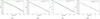 |
Fig. 2 Half-mass radius normalized to tidal radius as a function of mass predicted by the model (green line) for different model parameters. The dashed black like is the linear fit through Eq. (2) with its error band (gray shaded area). Panel a: model with |


3.1 Relationship of half-mass radius to stellar mass
As outlined in Sect. 2.1, the relation of the half-mass radius to the stellar mass is used to quantify the degree of segregation. This relationship is predicted by the model according to the input parameters. To describe the role of each parameter in shaping the rh(m) value, normalized to rt, we begin by considering a single power-law mass function. The slope α can assume two extreme values, −2 or 0, that is, a steep and a flat mass function, respectively. For the mass range, we keep mmin = 0.1 M⊙ as a fixed value and mmax = 100 M⊙ as a reference case. The minimum mass in GCs does not vary much during their evolution. Although masses slightly smaller than 0.1 M⊙ may be present, their exclusion does not affect our calculations, as we have checked. Actually, our results show that the mass range only plays a perceptible role when there is a large change from a broad range, covering three orders of magnitude in mass, to a narrower range of only one order of magnitude. This variation occurs mainly due to the maximum mass, which changes with the age of a stellar population. As time passes, the most massive stars evolve and eventually leave stellar remnants. Thus, stellar evolution alters the mass range, and it is important to account for this effect when studying the degree of segregation in any dynamical state. Current GCs have ages of ∼10 Gyr, with a star mass up to a maximum of the order of 1.0 M⊙. As a consequence, we also consider a maximum mass up to mmax = 1.0 M⊙ as a lower limit. Also, the value of Φ0 is expected to change with age. While current GCs show values of  (Teodori et al. 2024), it is expected that the initial phases of dynamical evolution are characterized by a lower Φ0. In our analysis, we consider
  for the aforementioned reference case, but we explore a wider range of
 ![Mathematical equation: ${{\rm{\Phi }}_0} \in [0.001,10]{\rm{ M}}_ \odot ^{ - 1}$](/articles/aa/full_html/2026/03/aa57469-25/aa57469-25-eq15.png) .
.
In Fig. 2 we show the most relevant cases where different model parameters change the predicted rh(m) profile. We also plot the corresponding fits with the linear relation in Eq. (2). In Table C.1, we report all the parameters explored and the corresponding linear fit results.
We consider the case  , α = 0.0, and mmax = 100 M⊙ given in Fig. 2a as a reference, where we obtain
  . The nonlinearity of the model prediction, which differs from a linear relation, is also evident from the plot; the linear relation, in turn, is only an indication of the rh(m) shape.
In Fig. 2b, we show the case with  , which is one order of magnitude less than the reference value. It corresponds to a β value that is one order of magnitude lower, which indicates a lower degree of segregation. In such a case, the linear regime is a very good approximation.
In Fig. 2c, a steeper mass function with α = −2.0 is used and provides a slightly larger value of β than in the reference case. The linear regime still follows well the slope of rh(m), indicating that a steeper mass function increases the segregation degree. However, as evident from Table C.1, we find that for other choices of the parameters, that is, a lower Φ0 or a lower mmax, the role of α is practically absent. Note that since realistic choices of parameters imply that a mmax = 100 M⊙ is more compatible with a low Φ0, while mmax = 1.0 M⊙ is related to a larger Φ0, the role of α is important in just a few cases. Indeed, for mmax = 1.0 M⊙ a different α only plays a role for  . On the contrary, for mmax = 100 M⊙, the slope α only changes β for
  , while for
  it has no effect. The results for
  cannot be considered relevant, as discussed later.
In Fig. 2d, we show the effect of a much smaller mass range, with mmax = 1.0 M⊙. The corresponding value of β is slightly lower than in the reference case, which indicates a lower degree of segregation. It is important to underline that the segregation degree is related to the relative spatial concentration of stars with different masses. Thus, it is the decreasing trend of rh(m)/rt and consequently its first derivative (β in the linear regime) that is relevant. On the contrary, the numerical values of rh(m)/rt are related to the global spatial concentration of stars and change with Φ0 as well as the slope and the maximum mass (giving a different q). This is evident in Fig. 3 that shows the half-mass radius to mass relationship predicted by the model for different input parameters. For a lower Φ0, the global half-mass radius is larger due to the weaker gravitational potential. A steeper mass function produces a more extended cluster, due to the poor number of massive stars compared to a flat mass function. Something similar occurs for a lower maximum mass. This is expected in multi-mass King-like models and recalls the relation between the model inputs and the concentration c = log(rt/rc) (Teodori et al. 2024).
Going back to the degree of mass segregation, the role of Φ0 looks immediately more important in changing β, with respect to the slope and maximum mass. As a consequence, in Fig. 4 we plot the relation between β and Φ0 for different choices of the slope of the mass function and the maximum mass.
For a more dynamically advanced equilibrium configuration, Φ0 increases and so does β, that is, the degree of mass segregation increases. However, for a subset of the obtained points, some considerations must be made regarding the explored parameters. Although we explored a wide range for all parameters, not all of them can be considered relevant for practical use or physically reasonable. First, the cases with  are not fully reliable, since the predicted rh(m) is strongly nonlinear at low masses (m < 0.5 M⊙), as shown in Figs. C.1a and C.1b. The trend for low-mass stars increases the resulting β, an effect that is less important if the maximum mass increases. The almost flat trend for m ≳ 0.5 M⊙ is more consistent for a smaller segregation, as we expect for a smaller Φ0 from the more regular trends in Fig. 4. Other indicators are the larger errors for β. As a consequence, the linear relation is not a good approximation for
  for any choice of the mass function parameters. The same problem is present for mmax = 1.0 M⊙ and
  , which again shows a nonlinear rh(m) in the low-mass stars regime, altering the β value as show in Fig. C.2a. Something similar also occurs for mmax = 10 M⊙ and
  , but here the effect on β is much smaller, as the nonlinear regime at low masses does not affect the fit, which is dominated by higher mass values (see Fig. C.2b).
Concerning physical validity, a low value of Φ0 corresponds to a low gravitational potential well. As in the case of the King single-mass model, solving the Poisson equation for a value of the equilibrium parameter W0 = m(φR − φ0)/(kBθ) that is too low is pretty difficult and is often avoided because of numerical problems in computing velocity integrals. In particular, there is a limit of W0 = 3.0 below which the clusters are not stable and are fated to disruption, since the total energy of the system is positive due to dominant tidal forces over self-gravity due to tidal forces dominating over self-gravity (Merafina 2017). This is related to a shallow gravitational potential well that is unable to keep stars together. In our model, we expect something similar, although a full description of stability for multi-mass models is still lacking (Merafina 2019). We expect that Φ0 is not the only responsible factor and that the mass function also plays a role. Thus, we can qualitatively state that values of Φ0 that are too low and mass ranges that are too small are not physically reasonable.
According to the values mentioned above for validity of the linear approximation, we can introduce W0,max = mmaxΦ0. Note that this is not the IC of the Poisson equation as defined in Teodori et al. (2024). According to this definition, the rh(m) relation loses linearity for W0,max ≲ 1.0. However, as mentioned above, the only exception is mmax = 10 M⊙ and  , where the nonlinear regime at low masses is not a serious problem to determine β. In addition, the lower limit also excludes the case when mmax = 1.0 M⊙ and
  for which rh(m) is linear, although this case has a pretty small potential well. These exceptions suggest that as the mass function becomes closer to the current observed mass ranges, the modeled rh(m) is well approximated by the linear relation for a slightly larger range of Φ0 values. However, we keep the lower limit to W0,max ≈ 1.0 as this likely provides more realistic values for the gravitational potential well.
We can also estimate an upper limit for the opposite regime, with a very large Φ0 and mmax. In this case, the gravitational potential is too strong and the predicted density profile is too steep and not physically reasonable for any dynamical state of GCs. In some cases, we are not even able to solve the equilibrium configuration. In the framework of the parent single-mass King model, this limit is related to the limit of the isothermal sphere (that is, W0 → ∞). Models with a very large equilibrium parameter are not physically reasonable because of the onset of the thermodynamic instability known as the gravothermal catastrophe. For the single-mass model, the critical value is W0 = 6.9 (Merafina 2017), beyond which the model starts losing its validity. The stability of GCs in the framework of the King model is well described by the caloric curve, which provides the aforementioned critical values for W0, as shown by Merafina (2017, 2018). It matches well the observed W0 distribution for Galactic GCs (Harris 1996) that does not show low-W0 values and peaks at the critical limit. The asymmetric shape of the distribution, steeper in the high-W0 regime, shows the onset of the gravothermal catastrophe, which leads to the collapse of the system on smaller timescales. Again, something similar should occur for a multi-mass King-like model. Unfortunately, we do not have an extension for the stability in such a case that can provide critical values for the parameters. Here, both the equilibrium parameter and the mass function are important. We can solve and obtain physically reasonable configurations for  and mmax = 1.0 M⊙, but not for mmax = 100 M⊙ or mmax = 10 M⊙. By using W0,max that we introduced before, we can infer an order of magnitude upper limit that is W0,max ∼ 10. It can be slightly higher if a steep mass function with α = −2.0 is considered.
According to the above discussion, to consistently solve the dynamical model, get an almost linear rh(m), and successfully generate stars (see later), we must choose input parameters such that 1.0 ≲ W0,max ≲ 10. However, we stress that the degree of segregation is mainly determined by Φ0, as the slope of rh(m) (namely β in the linear approximation) increases as Φ0 gets bigger.
According to what we outline here, a cluster that has a mass function with mmax = 100 M⊙ can be considered poorly segregated by setting  , while with
  , we have a higher degree of segregation. This would be representative of possible initial states of GC dynamical evolution that can be used as the ICs for N-body simulations (see Sect. 3.2). Note that here we can only define highly and poorly segregated cases in terms of a comparison of the associated Φ0 values (and the corresponding β). As
  is the lowest value for which the linear relation works, this determines the lowest segregation degree that our model can properly account for in the case of a typical IMF.
In contrast, a current state for GCs is characterized by mmax ∼ 1.0 M⊙ and we expect  depending on the segregation degree and its dynamical state. Note that
  is the order of magnitude obtained by comparing the model predictions on the degree of energy equipartition with current internal kinematics observations (Teodori et al. 2024). Thus, this latter case represents the highest degree of segregation that our model can consider.
As a consequence, the evolution of GCs should proceed from low Φ0 (but not too low) to higher Φ0, covering three to four order magnitudes and altering their mass functions (both slope and maximum mass) due to stellar evolution and evaporation. In Sect. 3.2, we further discuss reasonable choices for the model parameters to produce the ICs.
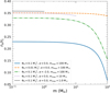 |
Fig. 3 Comparison of half-mass radius normalized to tidal radius as a function of stellar mass as predicted by the dynamical model for different input parameters. |
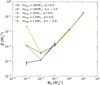 |
Fig. 4 Relation between Φ0 and β for different choices of the mass function slope, α, and maximum mass, mmax. The error bars indicate 1σ uncertainties. |
3.2 The generation of a primordially segregated cluster
As outlined in Sect. 2.2, the multi-mass King-like dynamical model offers a self-consistent way to properly distribute the positions, velocities, and masses of a stellar system. Here, we present the results of the adopted procedure, focusing mainly on the mass density and mean square velocity radial profiles, as well as the degree of mass segregation through the function rh(m).
As a reference case, we adopt  and a Kroupa-like mass function (Kroupa 2001), that is, a double power law with slope α1 = −1.3 for 0.1 ≤ m/M⊙ < 0.5 and α2 = −2.3 for 0.5 ≤ m/M⊙ ≤ 100. This case can be representative of the initial state of a cluster that lacks any relevant degree of segregation. As already outlined in Sect. 3.1, the successful generation of stars follows the same prescriptions regarding reasonable choices of input parameters.
To obtain the density, ρ, and mean square velocity, ⟨V2⟩, profiles of generated stars, we divided them into radial shells, and kept the number of stars within the shell constant. This ensured a similar statistical evaluation of the physical quantities. Each shell was defined by an inner and an outer radial coordinate. Their values were directly obtained from the stars within the shell, with the only exception being the innermost shell, whose minimum radius is the center. The shell was identified by a radial coordinate, r, which is the average of the aforementioned extremes. Concerning density, we summed the masses of the stars and normalized by the shell volume. For the mean square velocity, we averaged V2 within each shell. In Fig. 5, we show the mass density and the mean square velocity profiles for the reference model; these profiles resulted from the generation of N = 500 000 stars and the theoretical prediction of our model. For the analysis we used 5000 stars per radial shell and we computed the average mass within the shell to provide a qualitative visualization of mass segregation.
The generated stars represent the theoretical prediction well. The spread of points around the curve is related to the mass distribution and the choice of the number of stars per shell. The overall radial profiles can be considered as a weighted average of the profiles of each mass bin. In addition, the spread increases with a smaller number of stars for each radial shell.
Note that here the scaling to dimensionless units of generated stars is arbitrary, that is, we adopted reasonable scaling quantities to empirically estimate the central values (i.e., ρ0 and ⟨V20⟩) and the tidal radius from the generated points. This is needed to compare with the dimensionless profiles produced by the dynamical model. In Appendix B.1 we show that the generated profile matches the theoretical prediction for a lower number of stars, such as N = 50 000, which further supports the validity of our IC generation.
As expected for an equilibrium configuration with a low segregation degree, the points in Fig. 5 do not show a higher concentration of massive stars in the inner regions. On the contrary, a visual indication of mass segregation is evident in Fig. 6, where we report the density and mean square velocity radial profiles for the model with  and the same mass function as before, which represents a cluster with a higher segregation. The radial profiles were obtained with the same approach as described above. The generated stars again match the theoretical prediction well and we see that the inner shells show a slightly higher average mass, which is consistent with a higher degree of segregation. Note that this is only a qualitative insight as the value of the average mass is ruled by the adopted mass function, which has much more low-mass stars than massive stars.
However, it is more interesting to compare the degree of mass segregation through the function rh(m) for the two values considered for Φ0 and to check the behavior of generated stars with respect to the theoretical expectation. To estimate the relation of half-mass radius to mass for stars, we proceeded as described in Sect. 2.1.1 for the model. We first defined a grid of masses that is compatible with the model inputs. Due to the adopted mass function, the number of low-mass stars was much higher than that of massive stars. The previous approach for the radial profile, which uses a constant number of stars in each bin (here the mass bin), did not give a satisfying representation of the high-mass regime, the results for which are too poorly described. A better solution is obtained by choosing a grid that is uniformly spaced in logarithmic units. We selected stars that belong to each logarithmic mass bin, ∆m. Then, for each bin, we computed the cumulative mass radial profile, M(r, ∆m), and evaluated the half-mass radius of the mass bin by the condition M(rh, ∆m) = Mtot(∆m)/2 and by linearly interpolating over the radius. The cumulative radial profile for each mass bin was estimated as the density and mean square radial profiles, by defining radial shells that each had the same number of stars. In Fig. 7, we show the obtained rh(m) using 60 mass bins.
The case with a weak degree of segregation shows more massive stars that have an increasing dispersion with respect to the theoretical curve. This is related to the poor statistics at high masses. The procedure to obtain rh(m) needs to identify the cumulative mass profile for each mass bin, which is poorly populated for massive stars and thus has a rougher radial sampling. Conversely, the segregated case with  shows a clear decreasing trend, with a smaller dispersion in the high-mass regime compared to the
  case, but which is anyway larger than the low-mass regime. In Appendix B.1, we further discuss the correspondence between the generated stars rh(m) and the associated theoretical curve.
In the above description, we have considered all single stars. However, an important aspect in the generation of ICs concerns primordial binaries and, for evolved systems, stellar remnants. We provide a discussion for the latter in Sect. 3.3 and here we focus on primordial binaries.
We introduced the generation of ICs through our model as a consistent way to account for primordial mass segregation resulting from violent relaxation, which is a collisionless process. Thus, primordial binaries (formed before violent relaxation) behave like an object with a mass of m = m1 + m2, with m1 and m2 being the masses of the individual stars that make up the binary. As a consequence, when generating ICs with a nonzero binary fraction, the position and velocity of the center of mass must be associated to the mass m, rather than m1 and m2 separately, by means of our DF. The individual properties of each component are drawn from the center of mass properties and the adopted distribution for orbital parameters, which are not altered by our approach. In principle, the dynamical model should get a modified mass function as input that accounts for the dynamical mass of each object, rather than stellar mass. Binaries map objects belonging to lower-mass classes (m1 and m2 , respectively) onto the higher-mass class m. On average, this increases the number of dynamically massive objects and should be considered as an alteration of the input mass function to the dynamical model. Unfortunately, accounting for this effect means changing the mass function to a noncontinuous function, provided as an input to the model, which is currently not supported. However, as we outline in Sect. 3.1, variations in the shape of the mass function play a minor role in determining the segregation degree. Thus, we neglected this effect and tested the generation of ICs with primordial binaries. For the radial profiles, we obtain a correspondence between the generated stars and the theoretical curve that is as consistent as the correspondence for single stars, although to check the mean square velocity we must consider the center of mass velocity component, rather than individual ones that also account for the orbital motion. The same holds for rh(m), with stars following the prediction of the dynamical model well. Our tests reveal that this correspondence between model and generated stars works at any binary fraction, which we considered to be up to 50% of all the objects; that is, half of all stars are in binary systems.
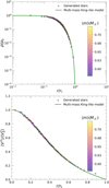 |
Fig. 5 Normalized mass density (upper panel) and mean square velocity (lower panel) radial profiles for N = 500 000 generated stars (circles) and the corresponding theoretical prediction (green line) for a model with |


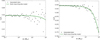 |
Fig. 7 Normalized half-mass radius as a function of stellar mass for generated stars (black circles) with the corresponding theoretical prediction (green line) for models with |


3.3 Initial conditions for multiple populations with a primordially segregated first generation
The dynamical evolution of MPs is a particularly intriguing case where primordial segregation may play a significant role. According to previous studies on violent relaxation, we expect FG stars to show a certain degree of primordial mass segregation. Our model provides a tool to set primordial segregation; this will be helpful for future works that consider the formation of SG stars in a segregated environment given by FG stars. Here, we focus on the technical aspect of generating a specific case for a segregated FG. In this way, we set the ICs to start dynamical evolution immediately after the formation of the SG. Firstly, we consider the case in which the SG is supposed to form when the FG age is 100 Myr, considering the asymptotic giant branch (AGB) scenario as the one responsible for the formation of the SG (D’Ercole et al. 2008; Calura et al. 2019). The main impact on the early cluster evolution is an alteration of the IMF and the stellar evolution effects on internal dynamics. Massive stars evolve faster and, when the SG form, we are mainly left with stars with masses up to ≈5 M⊙. In addition, we can have a fraction of FG stellar remnants, according to their retention in the cluster. This depends on the escape speed of the cluster and the kick velocity that is acquired by compact remnants as a result of supernova explosions. Kick velocities typically follow a Maxwellian distribution with a given velocity dispersion, which is a poorly constrained free parameter that is fixed to 190 km s−1 in the MCLUSTER code. With this choice, the FG can have massive remnants up to ≈25 M⊙.
Here stellar evolution and the formation of stellar remnants alter the mass function shape in the high-mass tail, reducing the number of objects, an aspect that also depends on the kick velocity. Thus, the inputs to the dynamical model must change accordingly, as for binaries. However, currently the model can only accept a continuous mass function, which prevents such a study. In any case, we expect that this variation only slightly affects the predictions and the degree of segregation, since alterations to the mass function play a minor role, as shown in Sect. 3.1. We present some tests concerning the effect of considering stellar remnants in ICs in Appendix B.2.
Note that the above discussion applies to remnants formed before the violent relaxation phase, so their dynamical state is well described by their mass, and we can use our model to produce ICs with primordial segregation. On the contrary, for remnants formed after the violent relaxation phase, their segregation pattern is better represented by the progenitor mass. Thus, in the generation of ICs for remnants, the progenitor mass should be used to describe the position and velocity, as the dynamical mass is what matters.
However, the topic is much more articulated as the timescale for stellar remnants formation depends on the progenitor mass, and, in particular for black holes and neutron stars, it may even occur during violent relaxation. In that case, remnants formed at different times need some time to adapt to the segregation pattern, a time that varies with mass. Therefore, the best way to characterize the effect of stellar remnants on the degree of primordial segregation is by appropriate simulations that include stellar evolution, which are largely beyond the scope of this work. This study may also reveal the dependence on the natal kick and provide an opportunity to study the retention of remnants in such a rapid dynamical process.
For these reasons, in the following we neglect the presence of remnants, and we keep the mass function slope constant and thus focus only on stars. We also assume the absence of primordial binaries, as we expect minor variations to β. Our goal is to explore the relationship between β and Φ0 specifically for a cluster with an age of 100 Myr.
3.3.1 The β–Φ0 relationship
From the perspective of exploring the effect of a different degree of primordial segregation in FG stars that have an age of 100 Myr, it is important to understand the possible choices for Φ0 and the corresponding β. The relation between Φ0 and β is shown in Fig. 8, for ![Mathematical equation: ${{\rm{\Phi }}_0} \in [0.01,{\rm{ }}2.0]{\rm{ M}}_ \odot ^{ - 1}$](/articles/aa/full_html/2026/03/aa57469-25/aa57469-25-eq43.png) . This range was selected in line with the discussion reported in Sect. 3.1, but considering a smaller lower limit. Accordingly, in Table 1 we report the estimated β. Figure 8 also reports a linear fit (dashed line):
. This range was selected in line with the discussion reported in Sect. 3.1, but considering a smaller lower limit. Accordingly, in Table 1 we report the estimated β. Figure 8 also reports a linear fit (dashed line):
 (3)
(3)
with a = 1.10 ± 0.02 and b = −1.83 ± 0.01.
Equation (3) and Fig. 8 result from practical use when setting the degree of primordial segregation for a population with an age of 100 Myr. Equation (3) links the empirical quantifier of the degree of segregation β, with the corresponding theoretical parameter Φ0 that identifies the equilibrium configuration of the dynamical model, used to generate the ICs.
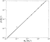 |
Fig. 8 Relation between β and Φ0 for a FG with an age of 100 Myr. The black dots are the obtained values from fits of rh(m) given in Table 1, while the dashed line is a linear fit log(β) = a log(Φ0) + b, with a = 1.10 ± 0.02 and b = −1.83 ± 0.01, with the corresponding error band (gray shaded area). |
Obtained values of β for different Φ0, for a FG with an age of 100 Myr.
3.3.2 The role of FG age
As we expect, a change in the FG age at the time of the SG formation converts into a different maximum mass, with minor effects on the degree of segregation with respect to variations in Φ0. As a confirmation of this general evidence, we explore how much Φ0 changes with age if we keep a constant degree of segregation through a fixed β. As a reference value, we consider the work by Livernois et al. (2021), which simulated violent relaxation, and obtain mass segregation showing the temporal evolution of rh/rJ for different mass bins, where rJ is the Jacobi radius. By taking the final stages (see their Fig. 9) and assigning an appropriate average mass to their mass bins, we built a rough rh(m) relation. It is mostly linear (see Fig. C.3) and yields a value of  . Then, we looked for values of Φ0 that yield the same β for different ages. Our findings are summarized in Table 2.
It is evident that the variations in Φ0 are small, as we expected. This also gives a reference value for Φ0 to be considered for primordial segregation. Note that it is of the same order of magnitude as our segregated case in previous sections, that is,  .
.
Obtained values of Φ0 for different ages of the FG, keeping the segregation degree with  fixed.
4 Conclusions
In this paper, we evaluate the degree of mass segregation through a multi-mass King-like dynamical model, which was already used to quantify the degree of energy equipartition (Teodori et al. 2024) in GCs.
Our main finding is the prediction of the relation of the half-mass radius to stellar mass, rh(m), which tracks and quantifies mass segregation and whose shape depends on the input parameters of the model. A linear approximation to rh(m) provides a good empirical estimate of the degree of mass segregation through the slope β. By fitting the prediction of the dynamical model with the linear relation, we characterize the role of each input parameter in changing the degree of segregation. We find that the gravitational potential well, through Φ0, is the main actor. A larger Φ0 produces a higher degree of mass segregation and shows a strong relation with β, which links the theoretical quantifier of the degree of segregation to the empirical one. However, to constrain β, direct measures of both stellar positions and masses are needed to estimate rh(m), while for Φ0 an indirect approach can also be used, such as fitting the surface brightness profile as discussed by Teodori et al. (2024). The mass function causes minor effects. A steeper mass function is associated with a slightly more important segregation as well as a larger maximum stellar mass, mmax.
We explored a wide range of Φ0 values and mass function parameters that are consistent with a cluster at early phases and current times. Our study reveals that to keep the linear approximation valid and to obtain a physically consistent quantity, we need to consider 1.0 ≲ W0,max ≲ 10, where W0,max = mmaxΦ0 is an auxiliary parameter that recalls the King-like shape of the DF. Thus, clusters at the beginning of their life have mmax ≈ 100 M⊙ and  , with the lower limit indicating poor segregation, while the upper shows a higher segregation degree. The degree of mass segregation increases with the dynamical age and thus current GCs are expected to have
  , which is compatible with the values found by Teodori et al. (2024).
We also show that the dynamical model allows for a self-consistent generation of ICs for N-body simulations. The DF fully characterizes the space of the positions, velocities, and masses. In particular, it offers a theoretical approach to set up a degree of primordial segregation. We present the properties of the generated stars by comparing with the corresponding model prediction for the density and mean square velocity radial profiles. We also show the behavior of rh(m) for generated stars with respect to the theoretical function, for different degrees of segregation. We obtain a good correspondence between the model and the generated stars in the range of parameters mentioned above. Furthermore, we check the scaling and convergence with the number of stars and the effect of fitting with the linear approximation the rh(m) obtained from stars.
We also discuss and verify the successful generation of clusters with primordial binaries. Here, our DF characterizes the position and velocity of the center of mass, according to the mass of the binary system, which better describes their early dynamical phase. During evolution, binaries can be considered as single objects that experience the global dynamical processes, although they can suffer disruption. However, since they are more massive than single stars, their degree of segregation at a given time will be higher. A quantification of this effect is given by the parameter A+, which is the area between the cumulative distribution of blue straggler stars and reference stars (Lanzoni et al. 2016; Ferraro et al. 2018). This quantity tracks the dynamical age of GCs and is expected to correlate with Φ0 (Teodori et al. 2024) and, consequently, with β.
Lastly, we account for MPs by considering a primordially segregated FG as resulting from the violent relaxation phase. In particular, we explored how an evolved FG can change Φ0 for a fixed degree of segregation through β. Then, we studied the relationship between β and Φ0 for the specific case of a FG with an age of 100 Myr at the time of the SG formation, as typically implied by the AGB pollution scenario. This is a good example of an interesting case for ICs that should be explored with N-body simulations. In this case, we consider and discuss the effects of stellar remnants in producing primordially segregated clusters, also exploring the retention of remnants and natal kicks. However, the topic is more articulated and requires attention as the timescales for stellar remnant formation can be similar to the violent relaxation timescale.
Our results further support the adoption of multi-mass models to consistently study the mass-based process in GCs, such as mass segregation and energy equipartition; this would provide a clearer understanding of the ESEV puzzle. The presence of MPs has increased interest in the formation and evolution of GCs. From this perspective, our work not only applies to present-day dynamical states but also offers a unique and consistent tool to shed light on the early phases of a GC’s life.
Acknowledgements
The authors thank the anonymous referee for the useful indications and comments that improved this paper.
References
- Alessandrini, E., Lanzoni, B., Ferraro, F. R., Miocchi, P., & Vesperini, E. 2016, ApJ, 833, 252 [NASA ADS] [CrossRef] [Google Scholar]
- Allison, R. J., Goodwin, S. P., Parker, R. J., et al. 2009, ApJ, 700, L99 [Google Scholar]
- Ascenso, J., Alves, J., & Lago, M. T. V. T. 2009, Ap&SS, 324, 113 [Google Scholar]
- Bastian, N., & Lardo, C. 2018, ARA&A, 56, 83 [Google Scholar]
- Baumgardt, H., & Makino, J. 2003, MNRAS, 340, 227 [NASA ADS] [CrossRef] [Google Scholar]
- Baumgardt, H., & Sollima, S. 2017, MNRAS, 472, 744 [Google Scholar]
- Baumgardt, H., De Marchi, G., & Kroupa, P. 2008, ApJ, 685, 247 [NASA ADS] [CrossRef] [Google Scholar]
- Beccari, G., Lützgendorf, N., Olczak, C., et al. 2012, ApJ, 754, 108 [NASA ADS] [CrossRef] [Google Scholar]
- Beccari, G., Dalessandro, E., Lanzoni, B., et al. 2015, ApJ, 814, 144 [Google Scholar]
- Binney, J., & Tremaine, S. 2008, Galactic Dynamics (Princeton University Press) [Google Scholar]
- Calura, F., D’Ercole, A., Vesperini, E., Vanzella, E., & Sollima, A. 2019, MNRAS, 489, 3269 [Google Scholar]
- Chandrasekhar, S. 1943, Rev. Mod. Phys., 15, 1 [CrossRef] [Google Scholar]
- Chandrasekhar, S. 1960, Principles of Stellar Dynamics (New York: Dover Publications, Inc.) [Google Scholar]
- Coenda, V., Baume, G., Palma, T., & Feinstein, C. 2025, A&A, 699, A15 [NASA ADS] [CrossRef] [EDP Sciences] [Google Scholar]
- Da Costa, G. S., & Freeman, K. C. 1976, ApJ, 206, 128 [NASA ADS] [CrossRef] [Google Scholar]
- Dalessandro, E., Ferraro, F. R., Massari, D., et al. 2015, ApJ, 810, 40 [NASA ADS] [CrossRef] [Google Scholar]
- Della Croce, A., Dalessandro, E., Livernois, A., et al. 2023, A&A, 674, A93 [NASA ADS] [CrossRef] [EDP Sciences] [Google Scholar]
- D’Ercole, A., Vesperini, E., D’Antona, F., McMillan, S. L. W., & Recchi, S. 2008, MNRAS, 391, 825 [CrossRef] [Google Scholar]
- Dib, S., & Henning, T. 2019, A&A, 629, A135 [NASA ADS] [CrossRef] [EDP Sciences] [Google Scholar]
- Dib, S., Schmeja, S., & Parker, R. J. 2018, MNRAS, 473, 849 [Google Scholar]
- Domínguez, R., Fellhauer, M., Blaña, M., Farias, J. P., & Dabringhausen, J. 2017, MNRAS, 472, 465 [CrossRef] [Google Scholar]
- Evans, N. W., & Oh, S. 2022, MNRAS, 512, 3846 [NASA ADS] [CrossRef] [Google Scholar]
- Ferraro, F. R., Lanzoni, B., Dalessandro, E., et al. 2012, Nature, 492, 393 [Google Scholar]
- Ferraro, F. R., Lanzoni, B., Raso, S., et al. 2018, ApJ, 860, 36 [NASA ADS] [CrossRef] [Google Scholar]
- Giersz, M., Leigh, N., Hypki, A., Lützgendorf, N., & Askar, A. 2015, MNRAS, 454, 3150 [Google Scholar]
- Gnedin, O. Y., & Ostriker, J. P. 1997, ApJ, 474, 223 [Google Scholar]
- Goodwin, S. P., & Whitworth, A. P. 2004, A&A, 413, 929 [NASA ADS] [CrossRef] [EDP Sciences] [Google Scholar]
- Gouliermis, D., Keller, S. C., Kontizas, M., Kontizas, E., & Bellas-Velidis, I. 2004, A&A, 416, 137 [NASA ADS] [CrossRef] [EDP Sciences] [Google Scholar]
- Gratton, R., Bragaglia, A., Carretta, E., et al. 2019, A&A Rev., 27, 8 [Google Scholar]
- Gunn, J. E., & Griffin, R. F. 1979, AJ, 84, 752 [NASA ADS] [CrossRef] [Google Scholar]
- Haghi, H., Hoseini-Rad, S. M., Zonoozi, A. H., & Küpper, A. H. W. 2014, MNRAS, 444, 3699 [NASA ADS] [CrossRef] [Google Scholar]
- Harris, W. E. 1996, AJ, 112, 1487 [Google Scholar]
- Hasan, P., & Hasan, S. N. 2011, MNRAS, 413, 2345 [Google Scholar]
- Hénon, M. 1961, Ann. Astrophys., 24, 369 [Google Scholar]
- Henon, M. 1969, A&A, 2, 151 [NASA ADS] [Google Scholar]
- Joshi, K. J., Nave, C. P., & Rasio, F. A. 2001, ApJ, 550, 691 [Google Scholar]
- Kerber, L. O., & Santiago, B. X. 2006, A&A, 452, 155 [NASA ADS] [CrossRef] [EDP Sciences] [Google Scholar]
- King, I. R. 1965, AJ, 70, 376 King, I. R. 1966, AJ, 71, 64 [Google Scholar]
- Kroupa, P. 2001, MNRAS, 322, 231 [NASA ADS] [CrossRef] [Google Scholar]
- Küpper, A. H. W., Maschberger, T., Kroupa, P., & Baumgardt, H. 2011, MNRAS, 417, 2300 [Google Scholar]
- Lanzoni, B., Ferraro, F. R., Alessandrini, E., et al. 2016, ApJ, 833, L29 [NASA ADS] [CrossRef] [Google Scholar]
- Leigh, N. W. C., Giersz, M., Marks, M., et al. 2015, MNRAS, 446, 226 [NASA ADS] [CrossRef] [Google Scholar]
- Livernois, A., Vesperini, E., Tiongco, M., Varri, A. L., & Dalessandro, E. 2021, MNRAS, 506, 5781 [NASA ADS] [CrossRef] [Google Scholar]
- Livernois, A. R., Vesperini, E., Varri, A. L., Hong, J., & Tiongco, M. 2022, MNRAS, 512, 2584 [NASA ADS] [CrossRef] [Google Scholar]
- Livernois, A. R., Aros, F. I., Vesperini, E., et al. 2024, MNRAS, 534, 2397 [Google Scholar]
- Lynden-Bell, D. 1967, MNRAS, 136, 101 [Google Scholar]
- Maschberger, T., & Clarke, C. J. 2011, MNRAS, 416, 541 [Google Scholar]
- McMillan, S. L. W., Vesperini, E., & Portegies Zwart, S. F. 2007, ApJ, 655, L45 [Google Scholar]
- Merafina, M. 2017, IJMPD, 26, 1730017 [Google Scholar]
- Merafina, M. 2018, Proceedings of XII Multifrequency Behaviour of High Energy Cosmic Sources Workshop — PoS(MULTIF2017), 306, 004 [CrossRef] [Google Scholar]
- Merafina, M. 2019, Proceedings of Frontier Research in Astrophysics III — PoS(FRAPWS2018), 331, 010 [CrossRef] [Google Scholar]
- Pang, X., Grebel, E. K., Allison, R. J., et al. 2013, ApJ, 764, 73 [NASA ADS] [CrossRef] [Google Scholar]
- Parker, R. J., & Goodwin, S. P. 2015, MNRAS, 449, 3381 [Google Scholar]
- Parker, R. J., Goodwin, S. P., Wright, N. J., Meyer, M. R., & Quanz, S. P. 2016, MNRAS Lett., 459, L119 [Google Scholar]
- Pavlík, V., & Vesperini, E. 2021, MNRAS Lett., 504, L12 [Google Scholar]
- Sollima, A. 2021, MNRAS, 502, 1974 [NASA ADS] [CrossRef] [Google Scholar]
- Sollima, A., & Baumgardt, H. 2017, MNRAS, 471, 3668 [NASA ADS] [CrossRef] [Google Scholar]
- Spitzer, L. 1987, Dynamical Evolution of Globular Clusters (Princeton University Press) [Google Scholar]
- Spitzer, L., & Härm, R. 1958, ApJ, 127, 544 [NASA ADS] [CrossRef] [Google Scholar]
- Šubr, L., Kroupa, P., & Baumgardt, H. 2008, MNRAS, 385, 1673 [CrossRef] [Google Scholar]
- Teodori, M., Straniero, O., & Merafina, M. 2024, A&A, 691, A202 [NASA ADS] [CrossRef] [EDP Sciences] [Google Scholar]
- Trenti, M., & van der Marel, R. 2013, MNRAS, 435, 3272 [NASA ADS] [CrossRef] [Google Scholar]
- Vesperini, E., & Heggie, D. C. 1997, MNRAS, 289, 898 [Google Scholar]
- Vesperini, E., McMillan, S. L. W., & Portegies Zwart, S. 2009, ApJ, 698, 615 [NASA ADS] [CrossRef] [Google Scholar]
- Vesperini, E., McMillan, S. L. W., D’Antona, F., & D’Ercole, A. 2013, MNRAS, 429, 1913 [Google Scholar]
- Vesperini, E., Varri, A. L., McMillan, S. L. W., & Zepf, S. E. 2014, MNRAS, 443, L79 [NASA ADS] [CrossRef] [Google Scholar]
- Vesperini, E., Hong, J., Webb, J. J., D’Antona, F., & D’Ercole, A. 2018, MNRAS, 476, 2731 [NASA ADS] [CrossRef] [Google Scholar]
- Vesperini, E., Hong, J., Giersz, M., & Hypki, A. 2021, MNRAS, 502, 4290 [NASA ADS] [CrossRef] [Google Scholar]
- Wang, L., Spurzem, R., Aarseth, S., et al. 2016, MNRAS, 458, 1450 [Google Scholar]
- Zhang, C., Li, C., de Grijs, R., et al. 2015, ApJ, 815, 95 [Google Scholar]
Appendix A Code documentation
In this section we summarize the main variations that we implement with respect to the public version of the MCLUSTER code, providing more operational details in addition to the procedure described in Sect. 2.2.
Concerning input parameters, we only introduce those associated with our dynamical model and keep the default choices, unless otherwise specified. Our main change is the inclusion of a function to distribute position and velocity components according to stellar mass and the DF in Eq. 1. As our multi-mass model is an extension of the King single-mass one, we take advantage of the existing function named “generate_king.” We add the inputs needed for the dynamical model, namely the mass function slopes, that is α for a single power-law mass function or α1 and α2 for a double power-law mass function (and a flag to distinguish between the two possible shapes), the mass extremes mmin and mmax, the Φ0 parameter and the number of mass classes used to define the grid of dynamical masses. The first task is responsible to run the multi-mass model with the aforementioned inputs. This separate program numerically integrates the Poisson equation for the gravitational potential, using a predictor corrector scheme. The solution provides the gravitational potential and the density radial profiles in dimensionless units. These quantities are used to obtain other radial profiles such as the mean square velocity, the cumulative mass and others. An important aspect lies in the description of mass-dependent quantities, namely physical properties associated to each mass. Indeed, after completion of the running command, our function loads some of these results, in particular M(r, m) which is normalized to its value at the edge, as well as the variables that appear in the DF in Eq. 1. The fundamental task is the generation of stellar positions and velocities. Here, for each stellar mass m we first search the corresponding lower and upper extremes in the mass grid of the dynamical model, such that mi < m < mi+1. This allows us to interpolate mass-dependent quantities such as k(m) and M(r, m), using the values on the grid of dynamical masses. Then, with the same random criterion used in the original “generate_king” function, we get the radius of the star according to M(r, m). Specifically, we extract a random number fmass between 0 and 1 and we iterate over radial coordinates until the value of the normalized M(r, m) is lower than or equal to fmass. Coordinates are given randomly assigning angles.
For velocities, the random approach is again similar to the original, that is using the kinetic energy distribution compatible with our DF. In particular, the maximum velocity allowed by the DF at the previously extract radius is obtained by the dimensionless potential. Thus, we iteratively extract a random velocity v between 0 and the maximum speed. If this yields a value of v2g(r, v, m) that is larger than or equal to a random number between 0 and the maximum of the DF associated to the star mass, the velocity is selected and, as for coordinates, its components are assigned by randomly extracting angles.
Appendix B Numerical tests
Here we show some tests with further analysis and discussion concerning the generation of stars.
B.1 Dependence on particle number N and convergence tests
In this section we show that generating stars with a lower number than adopted in the main text consistently yield main profile following the theoretical prediction. We show in Fig. B.1 the density and mean square velocity radial profiles for a cluster with N = 50 000 stars, adopting the same parameters in Sect. 3.2 and  (as in Fig. 5 for N = 500 000 stars). Here, we use 200 stars per shell and we do not report the points colored with the average mass within the shell as done to visualize mass segregation in the main text.
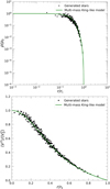 |
Fig. B.1 Normalized mass density (upper panel) and mean square velocity (lower panel) radial profiles for N = 50 000 generated stars (black circles) and the corresponding theoretical prediction (green line) for a model with |

The profile for generated stars well follows the theoretical prediction and confirms that our approach works also for a lower number of stars. This ensures that the subroutine that associates stellar mass, position and velocity according to the DF is reliable. The aforementioned correspondence is obtained also changing the number of stars per shell used to calculate the density and mean square velocity.
The same conclusion occurs for the relationship between the half-mass radius and the stellar mass, with rh(m) for generated stars well following the theoretical prediction. Naturally, for  the decreasing trend of rh(m) is less clear than for
  , because the number of massive stars is small and it even more difficult to estimate the half-mass radius for these stars. We show in Fig. B.2 the obtained quantities with the respective theoretical prediction. Here we use 10 mass bins.
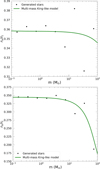 |
Fig. B.2 Normalized half-mass radius as function of stellar mass for N = 50 000 generated stars (black circles) with the corresponding theoretical prediction (green line) for models with |


In addition, we consider making a linear fit with Eq. (2) on rh(m) obtained from generated stars, providing the slope βgen. This can quantify the correspondence between the model and the generated objects, as βgen can be different from the theoretical one. This occurs because of the choice of the number of mass bins Nbin, whose optimal value changes with the number of stars. For N = 50 000 stars, 60 logarithmic mass bins used in the main text for N = 500 000 are not adequate. Indeed, the approach to evaluate rh(m) requires a sufficient number of stars in each mass bin to properly evaluate the cumulative mass radial profile. Our tests revealed that to appropriately evaluate rh(m) at different N, we must use 5 000 ≲ N/Nbin ≲ 10 000. Note that this quantity is only the average number of stars per bin, as we use logarithmic mass bins due to the shape of the mass function. The optimal N/Nbin ensures that βgen is close to the theoretical one. If this aspect is not considered, a systematic error much larger than the statistical one can be introduced. As an example, for N = 50 000 stars the best choices is N/Nbin = 5 000. A linear fit on the generated rh(m) gives  , compatible with the theoretical estimates of
  for a model with a Kroupa-like IMF with mmax = 100 M⊙ and
  .
.
Note that the uncertainty on the estimate of βgen decreases if the number of stars increases. We move from an average relative error of 10% for N = 50 000 to an average relative error < 5% for N = 500 000 stars, at least for  . On the contrary, for
  the uncertainties at low N are larger, around 20% if N = 50 000, but for higher N they converge to values similar to those obtained for a higher Φ0. We stress that these uncertainties are obtained by fitting the generated rh(m), while the fit to the theoretical prediction yields much lower errors on β.
In conclusion, the generation of stars well represents the underlying dynamical model adopted to distribute masses, positions and velocities regarding of the choice of N. In addition, to evaluate the segregation degree only empirically with the linear relation in Eq. 2, an optimal N/Nbin should be used to get a value of β more consistent with the theoretical prediction.
B.2 The effect of stellar remnants
Here we discuss some tests where we produce ICs for a cluster with 100 Myr accounting for stellar remnants. We consider that they are formed before violent relaxation, such that we can use the dynamical model to distribute position and velocity according to the remnant mass rather that the progenitor mass, as discussed in the main text. This allows us to use the same approach adopted for stars.
As a consequence, the density and mean square velocity profiles are not expected to show variations, as we verified. Here we focus on rh(m) obtained for generated objects with respect to the theoretical prediction, as remnants alter the mass function in the high-mass tail. The inputs to the dynamical model are varied only in terms of the maximum mass mmax, as only a continuous mass function can be provided in input. Thus, we neglect the slope variation in the high-mass tail.
If a cluster keeps all its remnants, due to low natal kicks, the maximum mass is higher and around ≈25 M⊙. On the contrary, a clusters losing all its remnants due to a high natal kick has all stars, whose maximum mass is ≈5 M⊙. The only variation that the theoretical β shows is related to mmax. On average, the relative variation between the two estimates of β is ≈10%. However, the generated rh(m) shows some differences, although it matches well the model prediction. The case with no remnant has all stars and no appreciable difference is seen in the ICs–model comparison. On the contrary, when considering all remnants we get a larger spread in rh(m) at high masses, due to the less number of objects in that range. This is even worse if we loose only some remnants. However, no significant variation is seen from the choice of a natal kick of ≈200 km/s if a different natal kick is considered (we explored values from 190 km/s to 260 km/s).
Concerning the estimate of βgen, obtained as a fit to the generated rh(m) with the linear relation in Eq. (2), as done in Sect. B.1, we first compared ICs keeping all remnants with ICs having the same maximum mass and IMF, but no age, thus all stars. Here, βgen for the first case has a much larger uncertainty, due to the spread at high masses. On average, the relative uncertainty is ≈30%, larger that for the second case, that is around ≈10%. The case with no age and all stars, together with the previous one of a cluster with 100 Myr and without remnants (whose mmax is lower), we find that βgen shows a larger relative uncertainty if mmax is lower. The reason is that with the absence of the high-mass regime the fluctuations at lower masses play a role, although they are significantly less than those at high-mass for cases with a higher mmax.
Appendix C Additional plots and explored parameters
Here we report some additional plots and the list of parameters explored in Sect. 3.1, given in Table C.1. In Fig. C.1 we show that for  the model prediction is strongly nonlinear in the low-mass regime, both for mmax = 1.0 M⊙ (Fig. C.1a) and mmax = 100 M⊙ (Fig. C.1b), with α = −2.0. The linear fit is not a good description and the corresponding β results higher than expected for a flatter trend, as in the high-mass regime. Similarly occurs for
  , α = 0.0 and mmax = 1.0 M⊙ and mmax = 10 M⊙ given in Fig. C.2, although the latter estimate of β is less affected by nonlinearity.
In Fig. C.3 we report values of rh(m) as obtained by Livernois et al. (2021) after the violent relaxation phase. We approximated the mass bins assigning an average mass. The trend results linear and the fit with Eq. (3) yields  .
.
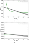 |
Fig. C.1 Half-mass radius normalized to tidal radius as function of mass for models with |


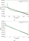 |
Fig. C.2 Half-mass radius normalized to tidal radius as function of mass for models with |


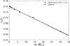 |
Fig. C.3 Half-mass radius – mass relationship as resulting from the final state of the violent relaxation work by Livernois et al. (2021, rough estimate), fitted with the linear relation in Eq. (2), yielding |

Explored model parameters and corresponding linear fit parameters.
All Tables
Obtained values of Φ0 for different ages of the FG, keeping the segregation degree with fixed.
All Figures
|
Fig. 1 ESEV puzzle schematic representation. |
| In the text | |
|
Fig. 2 Half-mass radius normalized to tidal radius as a function of mass predicted by the model (green line) for different model parameters. The dashed black like is the linear fit through Eq. (2) with its error band (gray shaded area). Panel a: model with |
| In the text | |
|
Fig. 3 Comparison of half-mass radius normalized to tidal radius as a function of stellar mass as predicted by the dynamical model for different input parameters. |
| In the text | |
|
Fig. 4 Relation between Φ0 and β for different choices of the mass function slope, α, and maximum mass, mmax. The error bars indicate 1σ uncertainties. |
| In the text | |
|
Fig. 5 Normalized mass density (upper panel) and mean square velocity (lower panel) radial profiles for N = 500 000 generated stars (circles) and the corresponding theoretical prediction (green line) for a model with |
| In the text | |
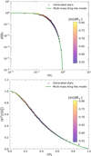 |
Fig. 6 Same as Fig. 5 but for |
| In the text | |
|
Fig. 7 Normalized half-mass radius as a function of stellar mass for generated stars (black circles) with the corresponding theoretical prediction (green line) for models with |
| In the text | |
|
Fig. 8 Relation between β and Φ0 for a FG with an age of 100 Myr. The black dots are the obtained values from fits of rh(m) given in Table 1, while the dashed line is a linear fit log(β) = a log(Φ0) + b, with a = 1.10 ± 0.02 and b = −1.83 ± 0.01, with the corresponding error band (gray shaded area). |
| In the text | |
|
Fig. B.1 Normalized mass density (upper panel) and mean square velocity (lower panel) radial profiles for N = 50 000 generated stars (black circles) and the corresponding theoretical prediction (green line) for a model with |
| In the text | |
|
Fig. B.2 Normalized half-mass radius as function of stellar mass for N = 50 000 generated stars (black circles) with the corresponding theoretical prediction (green line) for models with |
| In the text | |
|
Fig. C.1 Half-mass radius normalized to tidal radius as function of mass for models with |
| In the text | |
|
Fig. C.2 Half-mass radius normalized to tidal radius as function of mass for models with |
| In the text | |
|
Fig. C.3 Half-mass radius – mass relationship as resulting from the final state of the violent relaxation work by Livernois et al. (2021, rough estimate), fitted with the linear relation in Eq. (2), yielding |
| In the text | |
Current usage metrics show cumulative count of Article Views (full-text article views including HTML views, PDF and ePub downloads, according to the available data) and Abstracts Views on Vision4Press platform.
Data correspond to usage on the plateform after 2015. The current usage metrics is available 48-96 hours after online publication and is updated daily on week days.
Initial download of the metrics may take a while.