© The Authors 2026

1 Introduction

In the framework of the core accretion model, planets form in protoplanetary disks, where embryos first accrete planetesimals (Pollack et al. 1996) and pebbles (Ormel & Klahr 2010; Lambrechts & Johansen 2012; Kuwahara & Kurokawa 2020a,b). Once the proto-core exceeds approximately the mass of the Moon, it begins to gravitationally capture gas from its surroundings, forming an envelope. As long as the planetary mass is below the so-called critical core mass of approximately 10 M_⊕ (Earth masses), the envelope remains in near hydrostatic equilibrium. Beyond this critical mass, the planets undergo runaway gas accretion, evolving into gas giants.

In classical 1D models, the planetary envelopes are assumed to be static, isolated, and nearly spherically symmetric structures embedded in the disk (Mizuno 1980; Ikoma et al. 2000). However, recent 3D hydrodynamical simulations have revealed that envelopes are not closed systems but rather interact dynamically with the surrounding disk through a process known as recycling (e.g., Ormel et al. 2015b; Fung et al. 2015; Lambrechts & Lega 2017; Kuwahara et al. 2019).

These recycling flows enable a continuous gas exchange between the envelope and the disk, which could suppress the cooling and contraction of the envelope, thereby altering the timing and conditions under which runaway gas accretion occurs. Qualitatively, envelope growth is determined by the balance between heating and cooling. On the one hand, planetary cores grow via accreting solids, and the envelope heats up as the gravitational potential of the accreted solids is released. On the other hand, the envelope cools via radiation or convection, depending on its temperature gradient and ultimately on the opacity in the envelope (Rafikov 2006; Piso & Youdin 2014). Notably, previous works have shown that the efficiency of this recycling process strongly depends on the radiative cooling efficiency of the gas (Cimerman et al. 2017; Kurokawa & Tanigawa 2018; Moldenhauer et al. 2021).

The 3D dynamics of envelopes have further implications for the accretion of solids themselves. Gas flow around the planetary envelope directly affects the motion of particles smaller than approximately millimeter to centimeter in size in size (pebbles). Due to gas drag, the pebble accretion rate onto the planet is reduced by gas dynamics (Popovas et al. 2018; Kuwahara & Kurokawa 2020a,b; Okamura & Kobayashi 2021). Moreover, as solids enter the higher-temperature interior of the envelope, volatile species may sublimate and be advected along the gas flows through the envelope, thereby reducing the rate at which they are captured in the interior (Johansen et al. 2021; Wang et al. 2023).

Given these implications for the rates of gas and solid accretion onto embedded protoplanets, it is important to investigate envelope dynamics for a wide range of heating and cooling rates, which had not been previously done. Motivated by this, we present a comprehensive investigation into the response of the envelope to a wide range of heating and cooling rates. Because cooling efficiency depends on the opacity within the envelope, which is subject to large uncertainties, we adopted a simplified model that parameterizes radiative cooling efficiency.

The paper is structured as follows. Section 2 describes the numerical setup for our 3D hydrodynamical simulations that include accretion heating. In Sect. 3 we categorize the envelopes into three regimes, namely, fast, intermediate, and slow cooling regimes. We construct the analytic formulae of the mean flow speed within the envelope, and then model the recycling efficiency of small particles and vapors in the envelope (Sect. 4). Section 5 places our results in the context of previous work and discusses potential implications for envelope composition and planetary growth. We conclude in Sect. 6.

2 Numerical methods

We simulated the heating and cooling processes of a pebble-accreting planet embedded in a non-self-gravitating disk with the Athena++ code¹ (Stone et al. 2020). Our simulations were performed in spherical polar coordinates centered on a planet, where r is the distance from the planet, θ the polar angle, and φ the azimuth angle. We used the default numerical settings of Athena++, such as the integration schemes, unless otherwise specified.

Assuming a compressible, inviscid, and non-self-gravitating fluid, the Athena++ code solves the equation of continuity, the Euler equation, and the energy equation: $$\frac{\partial \rho }{\partial t}+\nabla ·\left(\rho \mathit{v}\right)=0,$$(1) $$\frac{\partial \left(\rho \mathit{v}\right)}{\partial t}+\nabla ·\left(\rho \mathit{v}\mathit{v}\right)=-\rho \nabla {\Phi }_{\mathrm{p}}-\nabla p+\rho ({\mathit{f}}_{\text{cor}}+{\mathit{f}}_{\text{tid}}),$$(2) $$\frac{\partial E}{\partial t}+\nabla ·\left[(E+p)\mathit{v}\right]=-\rho \mathit{v}·\nabla {\Phi }_{\mathrm{p}}+\rho \mathit{v}·({\mathit{f}}_{\text{cor}}+{\mathit{f}}_{\text{tid}})+Q_{\text{cool}}+Q_{\text{acc}}.$$(3) Here ρ is the density, v is the velocity, and p is the pressure. The total energy density is given by E=e+ρ v²/2 and the internal energy density by e=p/(γ−1), with γ=1.4 being the adiabatic index. The Coriolis and tidal forces are given by f_cor=−2e_z × v_g and f_tid=3xe_x−ze_z. We include the thermal relaxation and accretion heating terms, Q_cool and Q_acc, in the right-hand side of Eq. (3), which is described later in Sect. 2.1.

We implemented the gravitational potential of the planet as $${\Phi }_{\mathrm{p}}=-\frac{G{M}_{\mathrm{p}}}{r}\times f_{\mathrm{sm}}\times f_{\mathrm{inj}},$$(4) where G is the gravitational constant, and M_p is the planet mass. The smoothing function (f_sm) is given by (Fung et al. 2019) $$f_{\mathrm{sm}}=\frac{{(r-r_{\mathrm{in}})}^2}{{(r-r_{\mathrm{in}})}^2+r_{\mathrm{sm}}^2},$$(5) where r_in is the size of the inner boundary and r_sm is the smoothing length. We set r_sm=0.1 r_in (Zhu et al. 2021). This formulation (Eq. (5)) gives ∇ Φ_p=0 at the inner boundary, which is suitable for maintaining hydrostatic equilibrium. We note that a typical formula for a smoothed gravitational potential, ${\Phi }_{\mathrm{p}}=-G{M}_{\mathrm{p}}/\sqrt{r^2+r_{\mathrm{sm}}^2}$, leads to numerical heating, because of the nonzero gravitational force at the inner boundary (Appendix A).

The gravity of the planet is gradually inserted into the disk to prevent shock formation. Following Ormel et al. (2015a), we used the following injection function: $$f_{\mathrm{inj}}=1-exp[-\frac{1}{2}{\left(\frac{t}{t_{\mathrm{inj}}}\right)}^2],$$(6) where t is the time and t_inj=0.5 Ω⁻¹ is the injection time and Ω is the orbital frequency.

2.1 Cooling and heating terms

We treated the cooling of the gas as a thermal relaxation process. This was implemented as a source term of the energy equation, $$Q_{\text{cool}}=-\frac{e-e_0}{t_{\text{cool}}},$$(7) where e₀ represents the initial value. The isothermal and adiabatic limits are achieved when the cooling timescale approaches, respectively, t_cool → 0 and t_cool → ∞.

We considered an envelope heated by pebble accretion with a luminosity (Rafikov 2006; Lambrechts et al. 2014) of $$L\left(r\right)\approx \frac{G{M}_{\mathrm{p}}\dot{M}}{r_{\mathrm{in}}}(1-\frac{r_{\mathrm{in}}}{r})\equiv L_{\mathrm{acc}}(1-\frac{r_{\mathrm{in}}}{r}).$$(8) Here, we consider envelope heating due the accretion of solids at a mass rate Ṁ and neglect the other heat sources: the contraction of the envelope, the latent heat from evaporation, and the radioactive heating. The equation for the energy transportation is then given by $$\frac{\mathrm{d}L\left(r\right)}{\mathrm{d}r}=4\pi r^2{Q}_{\mathrm{acc}},$$(9) where Q_acc is the heating rate per unit volume. From Eqs. (8) and (9), we have $$Q_{\mathrm{acc}}=\frac{L_{\mathrm{acc}}}{4\pi }\frac{r_{\mathrm{in}}}{r^4}.$$(10) This expression is also used by Zhu et al. (2021), as it has the additional numerical benefit of no large intensity at the inner boundary. We confirmed that a jump appears in a temperature profile at the inner boundary when we consider the accretion heating only at the planet’s surface (Appendix A). The jump would lead to a large temperature gradient and hence to numerical convection.

2.2 Code units and simulation parameters

Our simulations were performed in the units of H=c_s=Ω= ρ₀=1, where H is the scale height, c_s is the isothermal sound speed, and ρ₀ is the midplane gas density at the planet orbital location, a_p. Since we neglect the self-gravity of the disk gas, we can introduce another normalization for the planetary mass, $$m\equiv \frac{R_{\mathrm{B}}}{H}=\frac{M_{\mathrm{p}}}{M_{\mathrm{th}}}\simeq 0.11\left(\frac{M_{\mathrm{p}}}{M_{\oplus }}\right){\left(\frac{M_{*}}{M_{\odot }}\right)}^{-1}{\left(\frac{0.03}{h}\right)}^3.$$(11) Here, $R_{\mathrm{B}}=G{M}_{\mathrm{p}}/c_{\mathrm{s}}^2$ is the Bondi radius, M_th=M_* h³ is the thermal mass, M_* is the stellar mass, h is the disk aspect ratio, M_⊙ is the solar mass. Finally, we parameterized the thermal relaxation timescale as the dimensionless quantity (Gammie 2001) $$\beta \equiv t_{\text{cool}}\Omega .$$(12)

In our simulation, we explored different solid accretion rates. The accretion luminosity (Eq. (8)) at the planetary surface r=R_p is on the order of $$L_{\text{surf}}=\frac{G{M}_{\mathrm{p}}\dot{M}}{R_{\mathrm{p}}}\sim {10}^{27}\mathrm{erg}/\mathrm{s}{\left(\frac{M_{\mathrm{p}}}{M_{\oplus }}\right)}^{2/3}\left(\frac{\dot{M}}{10M_{\oplus }/\mathrm{Myr}}\right).$$(13) The dimensionless accretion luminosity is then given by $$\begin{array}{rl}{\tilde{L}}_{\mathrm{a}\mathrm{c}\mathrm{c}}& =\frac{L_{\mathrm{s}\mathrm{u}\mathrm{r}\mathrm{f}}}{c_{\mathrm{S}}^2{M}_{\mathrm{t}\mathrm{h}}\mathrm{\Omega }}\\ & \simeq 1.1\times {10}^{-5}{\left(\frac{m}{0.1}\right)}^{5/3}{\left(\frac{{\rho }_{\mathrm{p}}}{5\mathrm{g}/{\mathrm{c}\mathrm{m}}^3}\right)}^{1/3}{\left(\frac{M_{\ast }}{M_{\odot }}\right)}^{-5/6}{\left(\frac{a_{\mathrm{p}}}{1\mathrm{a}\mathrm{u}}\right)}^{5/2}{\left(\frac{t_{\mathrm{a}\mathrm{c}\mathrm{c}}}{{10}^5\mathrm{y}\mathrm{r}}\right)}^{-1},\end{array}$$(14) where we used $$\frac{R_{\mathrm{p}}}{H}\simeq 1.4\times {10}^{-3}{\left(\frac{m}{0.1}\right)}^{1/3}{\left(\frac{{\rho }_{\mathrm{p}}}{5\mathrm{g}/{\mathrm{c}\mathrm{m}}^3}\right)}^{-1/3}{\left(\frac{M_{\ast }}{M_{\odot }}\right)}^{1/3}{\left(\frac{a_{\mathrm{p}}}{1\mathrm{a}\mathrm{u}}\right)}^{-1}.$$(15) Here ρ_p is the density of the planet. We defined the accretion timescale as t_acc ≡ M_p/Ṁ. For fiducial runs, we set t_acc=10⁵ yr, which corresponds to pebble accretion rates of Ṁ=10 M_⊕/Myr (Lambrechts et al. 2014). We also investigated low- and high-luminosity cases with t_acc=10⁶ yr and 10⁴ yr (corresponding to Ṁ=1 M_⊕/Myr and Ṁ=100 M_⊕/Myr); the latter case explores the upper end of possible solid accretion rates. The parameters of our simulations are summarized in Table 1.

2.3 Initial and boundary conditions, and resolutions

We assumed a vertically stratified density profile for the initial condition, $$\frac{\rho }{{\rho }_0}=exp[-\frac{1}{2}{\left(\frac{z}{H}\right)}^2].$$(16) A Keplerian shear flow is applied as an initial background velocity field, neglecting the headwind of the gas due to a global pressure gradient in a disk (see also Sect. 5.4). The initial velocity is given by $$\frac{\mathit{v}}{c_{\mathrm{s}}}=-\frac{3}{2}\frac{x}{H}{\mathit{e}}_y.$$(17)

We used a log-spaced grid in the radial coordinate ranging from r_in=10 R_p/H to r_out=10 R_B/H, which was divided into 256 grids. The polar and azimuth angles are uniformly divided into 40 and 160 grids.

The logarithmic grids have a higher resolution at the region close to the planet so that the Bondi radius is resolved by at least 118 grids in the radial direction. To save computational costs, the size of the inner boundary was arbitrarily determined to be r_in=10 R_p. We confirmed that the results hardly change when we adopted r_in=5 R_p (Appendix A).

For spatial reconstruction, we used a second-order piecewise linear method (PLM; xorder=2 in Athena++). In Appendix A we show the agreement between simulations using the PLM method and those using a higher-order method (a fourth-order piecewise parabolic method; xorder=3).

For the radial direction we set an inner reflecting boundary condition. At the outer boundary, we fixed the density and the velocity to the initial values. We only considered the upper half region of the disk, θ ∈ [0, π/2]. We used the a reflecting condition at the midplane, θ=0. On the pole we used the polar boundary condition, in which the physical quantities in the ghost cells are copied from the other side of the pole (Stone et al. 2020). We considered the full range of the azimuthal angle, φ ∈ [0, 2 π].

3 Numerical results

We find that the (thermo)dynamic states of planetary envelopes can be classified into three categories: the fast cooling (β< 1) regime, the intermediate cooling (1 ≲ β<1000) regime, and the slow cooling (β ≳ 1000) regime. The following sections (Sects. 3.1–3.3) describe the properties of the envelope in each regime for a fiducial run with m=0.1 and L̃_acc=1.1 × 10⁻⁵ (m/0.1)^5/3 (t_acc/10⁵ yr)⁻¹. The dependence on the planetary mass and the accretion luminosity will be presented in Sect. 3.4.

3.1 Fast cooling regime

When β ≲ 1, an envelope is nearly isothermal, corresponding to efficient radiative cooling. The shell-averaged density, temperature, and entropy profiles are in good agreement with the isothermal hydrostatic solution (Fig. 1). Here, the hydrostatic solution of the density is given by (e.g., Rafikov 2006) $${\rho }_{\mathrm{iso}}\left(r\right)\approx {\rho }_{0}exp\left(\frac{R_{\mathrm{B}}}{\sqrt{r^2+r_{\mathrm{sm}}^2}}\right).$$(18) Equation (18) is plotted in Fig. 1a (dashed line). In Fig. 1b we show the shell-averaged value of p/ρ, which is the measure of the temperature normalized by the value of the background disk, T₀. In this study, we defined the entropy function as $$\mathcal{S}\equiv \frac{p}{{\rho }^{\gamma }}.$$(19) The dashed line in Fig. 1c corresponds to $p_{\text{iso}}/{\rho }_{\text{iso}}^{\gamma }$, with $p_{\text{iso}}\equiv {\rho }_{\text{iso}}{c}_{\mathrm{s}}^2$ being the pressure of an isothermal envelope.

The envelope is convectively stable when the temperature gradient falls below the adiabatic gradient, $$\frac{\partial lnT}{\partial lnp}<{\nabla }_{\mathrm{ad}}\equiv \frac{\gamma -1}{\gamma }.$$(20) In the fast cooling regime, the temperature gradient is much smaller than the adiabatic gradient throughout the Bondi sphere (Fig. 1d).

The outer envelope, typically outside of 0.5 R_B, is subject to a recycling flow. Figure 2 shows the radial velocity of the gas and its dependence on β in both the x−y midplane and the x-z perpendicular plane. The gas, on horseshoe-like orbits, enters the Bondi sphere from the polar regions and exits through the midplane. This is referred to as the recycling flow (e.g., Ormel et al. 2015b; Fung et al. 2015; Kuwahara et al. 2019). However, the inner envelope remains bound to the planet with polar inflow unable to penetrate beyond a certain depth (Fig. 2, panel a and c). The isolation of the inner radiative layer from the recycling layer is clearly seen in the velocity vector shown in Fig. 3a. This aligns with previous simulations, without including accretion heating, that a positive entropy gradient (buoyancy force; Fig. 1c) suppresses the inflow penetrating the envelope (Kurokawa & Tanigawa 2018).

The boundary between the inner radiative and outer recycling layers depends on the cooling time β, and is typically located at approximately 0.5−1 R_B, shifting outward with increasing β. Figure 4 shows the numerically calculated recycling-radiative boundary (RRB) defined as $$\begin{array}{c}{r}_{\mathrm{R}\mathrm{R}\mathrm{B}}^{\mathrm{n}\mathrm{u}\mathrm{m}}\equiv max\{r\in [0,R_{\mathrm{B}}]\mid {⟨v_{\varphi ,\mathrm{mid}}⟩}_{\varphi }>max({⟨v_{r,\mathrm{mid}}⟩}_{\varphi },{⟨v_{\theta ,\mathrm{mid}}⟩}_{\varphi })\\ \wedge {\mathrm{\nabla }}_{\text{shell\hspace{0.17em}}}<0.95{\mathrm{\nabla }}_{\mathrm{a}\mathrm{d}}\}\end{array}$$(21) Here 〈 v_{i, mid}〉_φ is the azimuthally averaged velocity at the midplane and ∇_shell is the shell-averaged value of ∂ ln T/∂ ln p. The first condition on the right-hand side of Eq. (21) corresponds to the dynamical definition of a bound atmosphere (Moldenhauer et al. 2022). The factor of 0.95 in the second condition is a safety factor for the numerically determined temperature gradient ∇_shell (Fig. 1d). The orange squares in Fig. 4 mark $r_{\text{RRB}}^{\text{num}}$ for the fiducial run with m=0.1. A fitting formula for $r_{\text{RRB}}^{\text{num}}$ is given in Appendix B (dashed orange line in Fig. 4).

The mean flow speed in the radiative layer is characterized by the shear flow at its outer edge and reaches approximately 1 to 10% of the sound speed, depending on β (Fig. 5). Further outside the envelope, r ≫ R_B, the flow is dominated by the Keplerian shear, the hemispherically averaged value of which is given by $$\frac{{\langle v_{\mathrm{sh}}\rangle }_{\mathrm{shell}}\left(r\right)}{c_{\mathrm{s}}}=\frac{{\int }_0^{2\pi }{\int }_0^{\pi }\frac{3}{2}{r}^3\Omega {sin}^2\theta |cos\varphi |\mathrm{d}\theta \mathrm{d}\varphi }{{\int }_0^{2\pi }{\int }_0^{\pi }{r}^{2}sin\theta \mathrm{d}\theta \mathrm{d}\varphi }\frac{1}{c_{\mathrm{s}}}=\frac{3}{4}\frac{r}{H}.$$(22) In Fig. 5, the predicted mean flow speeds from Eq. (22) are shown by the dashed lines for β=0.01 and 1, assuming that the outer edges of the radiative layer are r=0.3 R_B and 0.8 R_B, respectively. These predictions are consistent with the numerical results. The mean flow speed is lowest at the boundary between the radiative and recycling layers and converges to the Keplerian shear beyond the Bondi radius (Fig. 5).

We show the shell-averaged radial and azimuthal velocities in Fig. 6. The envelopes rotate in the prograde direction, opposite the direction of the shear flow. We do not see the development of a circumplanetary disk: the rotational velocity of the envelope is much smaller than the Keplerian velocity. The formation of a prograde-rotating envelope can be attributed to the influence of the Coriolis force on the 3D gas flow (Ormel et al. 2015b).

The azimuthal velocity dominates in the radiative layer (the solid lines in Fig. 6), peaking near the inner boundary and decreasing outward.

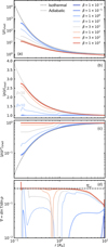Fig. 1 Shell-averaged density, temperature, entropy, and temperature gradient (from top to bottom) for different β values. We set m=0.1 and Ṁ=10 M⊕/Myr. All panels are the snapshots at the end of the calculation, t=50. The dashed and dotted curves in panels a–c are the analytic models given by Eqs. (18), (25), and (26). The horizontal dashed line in panel d is the adiabatic gradient, Eq. (20).

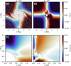Fig. 2 Radial velocity of the gas as a function of cooling time (β). We set m=0.1 and Ṁ=10 M⊕/Myr. All panels are snapshots at the end of the calculation, t=50. The dashed circle denotes the Bondi radius. Top: midplane slices, with streamlines shown in panel a. Bottom: vertical slices where the velocity is hemispherically averaged in the azimuthal direction, φ ∈[−π/2, π/2].

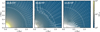Fig. 3 Hemispherically and time-averaged density and velocity vector on the vertical slice. We set m=0.1. The physical quantities are averaged over the azimuth and the time, φ ∈[−π/2, π/2] and t ∈[40, 50]. The dashed white circle in the top panels is the Bondi radius of the planet.

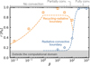Fig. 4 Boundary between the recycling and radiative layers (orange) and the radiative and convective layers (blue), as a function of cooling time (β). The squares and circles are the numerical results, obtained for m=0.1 and Ṁ=10 M⊕/Myr. The dashed lines are the fitting formulae (Appendix B). The hatched region is not probed by our simulations.

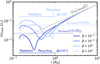Fig. 5 Shell-averaged mean speed for β=10−2−101. We set m=0.1 and Ṁ=10 M⊕/Myr. This figure shows the state at the end of the simulation, t=50. The radiative and recycling layers are qualitatively indicated. The horizontal dotted lines correspond to Eq. (22) with r=0.3 RB and r=0.8 RB. The dashed-dotted gray curve represents Eq. (22).

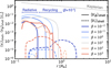Fig. 6 Shell-averaged radial velocity (solid lines) and azimuthal velocity (dashed lines), for different β. Negative components are omitted. We set m=0.1 and Ṁ=10 M⊕/Myr. The dotted gray line represents the Keplerian velocity around the core.

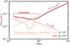Fig. 7 Same as Fig. 5 but for β=102 and 103. The convective, radiative, and recycling layers are qualitatively indicated. The dashed red and yellow curves show Eq. (24), under the assumptions of fully and partially convective envelopes with lm=RB and lm=0.2 RB, respectively.

3.2 Intermediate cooling regime

This regime (1 ≲ β ≲ 300) features a three-layer envelope structure with, from inside to outside, a convective, radiative and recycling layer (Fig. 3b; Lambrechts & Lega 2017). The shell-averaged envelope properties – temperature, density, and entropy – lie between isothermal and adiabatic profiles (Figs. 1a–c). As β increases, the entropy gradient flattens (Fig. 1c), allowing polar inflow to penetrate deeper (Figs. 3a and b).

Similar to the near-isothermal envelopes, the outer shells are dominated by Keplerian shear penetrating the envelope. However, deeper inside the envelope we notice convection motions bound to the inner envelope, when 30 ≲ β ≲ 300 (Fig. 3b). The blue circles in Fig. 4 mark the numerically-calculated radiative-convective boundary (RCB), $$r_{\mathrm{RCB}}^{\mathrm{num}}\equiv max\{r\in [0,R_{\mathrm{B}}]\mid {\nabla }_{\mathrm{shell}}\ge 0.95{\nabla }_{\mathrm{ad}}\},$$(23) while the dashed blue line shows the corresponding fitting formula (see Appendix B). In Appendix C we present an analytic model to calculate the shell-averaged mean flow speed in the convective layer, which is in good agreement with the numerical results (Fig. 7). When the energy is transported by convection, in the framework of mixing length theory, the characteristic speed of convection is given by (Appendix C) $$\frac{v_{\mathrm{con}}(r,l_{\mathrm{m}},{\tilde{L}}_{\mathrm{acc}})}{c_{\mathrm{s}}}\approx {\left(\frac{{\nabla }_{\mathrm{ad}}}{8\pi {(r/H)}^3}\frac{(l_{\mathrm{m}}/R_{\mathrm{B}}){\tilde{L}}_{\mathrm{acc}}}{{\rho }_{\mathrm{ad}}\left(r\right)/{\rho }_0}\right)}^{1/3}.$$(24) Here, l_m is the mixing length corresponding to the size of the convective cell. The convective flow speed is fastest near the inner boundary and decreasing outward (Eq. (24); Fig. 7). The maximum convective flow speed reaches a few percent of the sound speed. The mean flow speed drops by an order of magnitude in the radiative layer, then increases in the recycling layer due to the subsonic polar inflow and midplane outflow.

3.3 Slow cooling regime

When β ≳ 1000, the envelope is fully convective (Fig. 2, panel b and d). No steady-state flow can be identified within the envelope and material isotropically enters and leaves the envelope (Fig. 3c). Nevertheless, the shell-averaged density, temperature, and entropy (Figs. 1a–c) match the 1D analytic adiabatic limit (e.g., Rafikov 2006): $${\rho }_{\mathrm{ad}}\left(r\right)\approx {\rho }_0{(1+{\nabla }_{\mathrm{ad}}\frac{R_{\mathrm{B}}}{\sqrt{r^2+r_{\mathrm{sm}}^2}})}^{1/(\gamma -1)},$$(25) $$T_{\mathrm{ad}}\left(r\right)\approx T_0(1+{\nabla }_{\mathrm{ad}}\frac{R_{\mathrm{B}}}{r}).$$(26) The temperature gradient matches the adiabatic one throughout the Bondi sphere (Fig. 1d).

Flow speeds in the convective envelope now reach approximately 10% of the sound speed (Fig. 7). This is in agreement with Eq. (24). Larger mixing lengths and lower densities compared to the intermediate regime lead to higher convective velocities, as predicted by Eq. (24), v_con ∝(l_m L/ρ)^1/3. This vigorous convection influences material transport, which is explored further in Sect. 4.

3.4 Planetary mass and luminosity dependence

Envelope dynamics are controlled by the balance of heating and cooling. A higher accretion luminosity steepens the temperature gradient, promoting convection. In practice, the accretion luminosity depends on planetary mass and pebble accretion rate (Eq. (8)). Therefore, we varied the accretion rates by two orders of magnitude (Table 1). From these numerical experiments, we observe that the critical β that separates the slow cooling regime from other regimes depends on the accretion luminosity. As shown in Fig. 8a, full convection occurs when β ≥ 10³ and Ṁ ≤ 10 M_⊕/Myr, but already at shorter cooling times (β ≥ 10²) when Ṁ=100 M_⊕/Myr. However, the structure of the envelope does not change significantly with variations in the accretion luminosity. We do note that the shell-averaged mean speed within the Bondi radius increases with the accretion luminosity, as can be seen in Fig. 8b, as expected from Eq. (24). Finally, in the current work, we briefly explored the dependence on planetary mass. We varied the planetary masses within a factor of three. As expected, varying the planetary mass within a factor of three does not lead to substantial changes in the envelope structure (Fig. 9).

4 Tracing material transport

Envelope dynamics strongly influence the transport of small particles and vapors. To get an insight into material transport within the envelope, we used passive scalars as tracer particles in our hydrodynamical simulations that obey the following transport equation (Stone et al. 2020): $$\frac{\partial \rho C_{\text{tracer}}}{\partial t}+\nabla ·\left[\rho \mathit{v}{C}_{\text{tracer}}\right]=0.$$(27) We kept the passive scalar density C_tracer equal to the gas density when t< t_tracer,0. After t ≥ t_tracer,0, the passive scalar density varies in time with the gas motion. We set t_tracer,0=5 Ω⁻¹. A reflecting inner boundary condition is applied to the passive scalars. For the outer boundary condition, we set the passive scalar density equal to 0 at r>0.8 r_out, where r_out is the outer edge of the simulation domain (Sect. 2).

Figure 10 shows the tracer concentration in the x-y midplane for different cooling times, while Fig. 11 illustrates the distribution in the x-z perpendicular plane. Tracers are confined within the radiative layer, which is isolated from the outer recycling layer by buoyancy. Outside the radiative layer, tracers are efficiently transported by recycling, shear, and horseshoe flows (the top rows in Figs. 10 and 11a). Even if a convective layer lies beneath a radiative one, tracers remain trapped in the radiative layer (the middle rows in Figs. 10 and 11b). However, in a fully convective envelope, tracers are expelled within a few tens of orbits (the bottom rows in Figs. 10 and 11c).

We further explored the time evolution of the tracer concentration as a function of radius in the envelope, for different cooling times. Figure 12 shows the tracer density in different radial zones as a function of orbital time. For the short β-cooling times (β ≲ 1), the tracer concentration remains nearly constant within the radiative layer, r ≲ 0.6−0.8 R_B, decaying only in the outer recycling zone (Fig. 12a). In the intermediate cooling regime, 1 ≲ β ≲ 300, in which the inner envelope can be partially convective, the tracers stagnate in the innermost part of the envelope, r ≲ 0.4−0.6 R_B (Fig. 12b). In the slow cooling regime, β ≳ 1000, the tracer concentration drops rapidly throughout the fully convective envelope (Fig. 12c).

The evolution of the tracer concentration at a radius r in the envelope is well described by a simple exponential decay: $${\rho }_{\mathrm{tracer}}^{\mathrm{model}}(r,l_{\mathrm{m}},{\tilde{L}}_{\mathrm{acc}},t)={\rho }_{\mathrm{tracer},0}\times exp(-\frac{t-t_{\mathrm{tracer},0}}{\tau (r,l_{\mathrm{m}},{\tilde{L}}_{\mathrm{acc}})}),$$(28) where τ corresponds to the characteristic timescale to transport the tracers in the convective or radiative layer. The above equation is plotted in Figs. 12b and c with the orange lines, reproducing the numerical results. Here we define $$\tau (r,l_{\mathrm{m}},{\tilde{L}}_{\mathrm{acc}})\equiv \{\begin{array}{c}\frac{2l_{\mathrm{m}}}{v_{\mathrm{con}}(r_{\mathrm{in}},l_{\mathrm{m}},{\tilde{L}}_{\mathrm{acc}})}(\text{when}{l}_{\mathrm{m}}=R_{\mathrm{B}}),\hfill \\ \frac{R_{\mathrm{B}}-r}{v_{\mathrm{rad}}}(\text{when}0<l_{\mathrm{m}}<r<R_{\mathrm{B}}),\hfill \\ \infty (\text{when}r\le l_{\mathrm{m}}<R_{\mathrm{B}}\text{or}{l}_{\mathrm{m}}=0),\hfill \end{array}$$(29) where v_rad is the mean flow speed in the radiative layer. When m=0.1, Eq. (29) yields τ ≈ 3 Ω⁻¹ for a fully convective envelope, where the mixing length is comparable to the Bondi radius (l_m=R_B), using Eq. (24) for v_con. For a partially convective envelope, we find that at depth of r=0.4 R_B τ ≈ 30 Ω⁻¹, taking l_m=0.2 R_B. These estimates rely on the following assumptions: (1) In a fully convective envelope, tracers are circulated over a distance of 2 l_m (circulation in a convective cell), regardless of their initial position. (2) When the envelope has inner convective and outer radiative layers, tracers are transported outward in the radiative layer at a speed of v_rad=0.1 v_con(r, l_m, L̃_acc), inferred from Fig. 7. (3) In a near-isothermal envelope, the tracers are effectively trapped. We note that even in a fully radiative envelope, radial velocities are small but finite (10⁻⁵ c_s; Fig. 6), which implies a Bondi-crossing timescale exceeding 10⁴ orbits for a planet with m=0.1.

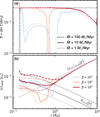Fig. 8 Shell-averaged temperature gradient and mean velocity for different β values and accretion luminosities. All panels are the states at the end of the calculation, t=50. The dashed, solid, and dotted gray curves in panel b are given by Eq. (24) with an assumption of fully convective envelopes (lm=RB). Thus, these gray lines should be compared with the red lines. The dashed-dotted gray curve is given by Eq. (22).

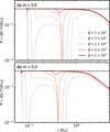Fig. 9 Shell-averaged temperature gradient for different planetary masses and β values. We set Ṁ=10 M⊕/Myr. All panels are the snapshots at the end of the calculation, t=50. The horizontal dashed line is the adiabatic gradient, Eq. (20).

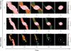Fig. 10 Tracer concentration at the midplane. We set m=0.1. Different rows correspond to different β values (β=100, 102., and 103, from top to bottom). Different columns correspond to different times (t=15, 20, 25, 30, and 50 in code units, from left to right).

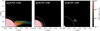Fig. 11 Tracer concentration in the x-z plane at the end of the calculation (t=50 in code units), after a hemispherical average along the azimuthal direction.

5 Discussions

5.1 Model limitation: β-cooling assumption

The β-cooling model employed in this study is a simplified radiative cooling model (e.g., Gammie 2001). Assigning a fixed β value throughout the envelope is an assumption that does not take into account that the primary source of opacity are small dust grains present in the envelope. In Appendix D we show that the applicability of the β-cooling model is valid when the opacity is low κ ≲ 10⁻⁵−10⁻⁴ cm²/g or at distances outside of ≳ 10 au. However, there is significant uncertainty in the opacity of planetary envelopes. The primary source of opacity is dust, and a commonly adopted value is κ ∼ 1 cm²/g, corresponds to that of the interstellar medium. However, processes such as dust growth and settling can substantially reduce dust opacity, potentially resulting in values much lower than the interstellar medium standard (Ormel 2014; Mordasini 2014). Notably, in the region within ≲ 0.1 R_B, the opacity can drop to values as low as κ ≲ 10⁻⁴ cm²/g because of dust coagulation.

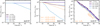Fig. 12 Time evolution of the shell-averaged tracer concentration for β=100 (panel a), 102 (panel b), and 103 (panel c). Different colors correspond to different shell radii. The orange lines are given by Eq. (28). In panel b we set lm=0.2 RB (partially convective) and plot the decay rate at r=0.4 RB (the solid line), r=0.6 RB (the dotted line), and r=0.8 RB (the dashed line), respectively. In panel c, we set lm=RB (fully convective).

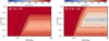Fig. 13 Analytic estimate of the envelope’s cooling time as a function of the opacity and the RCB location. Different panels correspond to different orbital locations of the Earth-mass planet.

5.2 Analytic estimate of the envelope’s cooling time

The orbital location of the planet determines the effective cooling rate of the envelope. In Appendix E we provide an analytical estimate of the envelope’s cooling time, β_env, by combining the cooling time of the background disk gas – which constrains the cooling time at the outer edge of the envelope – with the depth-dependent cooling time derived from a two-layer envelope model. The cooling time of the background disk gas, β_disk, takes into account radiative cooling from the disk surface and in-plane cooling (radial thermal diffusion through the disk midplane; Ziampras et al. 2023). The cooling time derived from the two-layer model, β_RCB, is the time it takes to cool the envelope until the RCB reaches a given pressure depth (Piso & Youdin 2014). Figure 13 shows that, in the deep envelope (r ≲ 0.1 R_B) that is not directly probed by our simulations, the cooling time exceeds 10³ orbits, with only a weak dependence on the dust opacity. In contrast, in the outer envelope (≳ 0.1 R_B), cooing times can be around 100 orbits for Earth-like planets in the inner disk (1 au; Fig. E.7a), but decreasing with orbital radius to 1−100 orbits outside of 10 au (Fig. E.7b). This indicates that, envelopes will generally be in the fast or intermediate cooling regime in the outer disk, while this breaks down toward the inner disk where cooling timescales are long. There, planets approaching the Earth to super-Earth regime, would acquire fully convective envelopes. This would hamper further growth, as such low-mass envelopes have long growth timescales (Lambrechts & Lega 2017) and even pebble accretion rates can be reduced (see Sect. 5.6).

Our simulations primarily cover the domain outside 0.1 R_B, where the cooling time is mainly set by β_disk. If the opacity κ is approximately constant in this region, then β_env is also constant throughout the domain (Fig. 13), in line with a the uniform β value in our simulation domain. However, the opacity within the envelope can vary by several orders of magnitude due to processes such as dust growth and settling (Ormel 2014; Mordasini 2014). Moreover, gas dynamics can cause the opacity to vary not only radially, but also vertically and azimuthally, resulting in 3D variations within the envelope (Krapp et al. 2022). The coevolution of dust and the envelope is further discussed in Sect. 5.7.

5.3 Comparison to previous studies

Numerous simulations of the envelopes of embedded planet have been conducted, both with and without accretion luminosity. In this section we first compare our results with previous studies that neglect accretion luminosity (Sect. 5.3.1), followed by those that include it (Sect. 5.3.2).

5.3.1 Without accretion luminosity

Although neglecting the accretion luminosity is an unrealistic assumption and requires careful treatment in numerical simulations (Zhu et al. 2021), it remains a convenient simplification and has been widely adopted in previous studies.

In the isothermal limit, where buoyancy forces are absent, polar inflow can penetrate deep into the envelope resulting in a structure dominated entirely by the recycling layer (Ormel et al. 2015b; Fung et al. 2015; Kuwahara et al. 2019). As shown in Fig. 4, smaller values of β lead to radially wider recycling layers, consistent with these earlier findings. In our simulations, the lower bound of the cooling time is β=0.01; we expect that even smaller β would reproduce the isothermal limit.

In reality, envelopes have a finite cooling time. Using the β-cooling model with β ≤ 1, Kurokawa & Tanigawa (2018) conducted 3D hydrodynamic simulations and found that the radiative layer is isolated from the recycling layer due to a buoyancy force, and that its extent increases with β. This is consistent with our results (Fig. 4).

In the absence of convection, envelope recycling is more efficient in the outer envelope regions, a trend consistently observed in both isothermal and non-isothermal envelopes (Ormel et al. 2015b; Cimerman et al. 2017; Béthune & Rafikov 2019; Moldenhauer et al. 2021; Bailey & Zhu 2024). Cimerman et al. (2017) performed 3D radiation hydrodynamic simulations using the flux-limited diffusion (FLD) approximation for Earthlike planets, assuming a low opacity (κ=10⁻⁴−10⁻² cm²/g). They showed that the outer envelope (r ≳ 0.4 R_B) recycles within approximately 1−10 orbits, while the inner regions recycle over approximately 100 orbits. A subsequent study confirmed that the entire envelope recycles over finite timescales, even if the inner radiative layer is isolated from recycling (Moldenhauer et al. 2022). Moldenhauer et al. (2022) reported that the bulk of the envelope recycles on a timescale of approximately 10² orbits, except for regions extremely close to the planetary surface, where timescales can be as long as 10⁴ orbits. Although the physical mechanism remains unclear, the authors noted that the envelope becomes turbulent, which enables even deeply embedded tracers to eventually escape. In contrast, our results suggest lower recycling efficiency in the inner envelope. As discussed in Sect. 4, the recycling timescales in the radiative layer can exceed 10⁴ orbits. No prominent turbulence is observed in the radiative layer. Since hydrostatic equilibrium is established, radial velocities remain very small (Fig. 6). A recent simulation solving the radiative transfer equations has also confirmed that the inner envelope (r<0.4 R_B) remains insulated from recycling (Bailey & Zhu 2024), consistent with our findings.

The efficiency of recycling in the radiative interior continues to be a matter of debate, especially in light of the diversity of numerical treatments across different models. In regions near the inner boundary, where density and pressure gradients become steep, either a high numerical resolution or large gravitational smoothing lengths are required to maintain hydrostatic balance (Zhu et al. 2021). Insufficient resolution in these regions leads to artificial velocity fluctuations and numerical heating, which affects the entire envelope (Ormel et al. 2015b; Zhu et al. 2021). Furthermore, Zhu et al. (2021) noted that an explicit luminosity input is required to accurately model the envelopes. Therefore, the accretion luminosity should not be neglected.

5.3.2 With accretion luminosity

The envelope of an embedded planet is inherently heated by accretion of solids and compressional heating of the gas, resulting in intrinsic luminosity. Several sophisticated radiation-hydrodynamic simulations of envelopes have been carried out so far. Lambrechts & Lega (2017) performed 3D radiation hydrodynamic simulations using the FLD approximation and found that the envelope exhibits a three-layer structure: the convective, radiative, and recycling layers from inside out. Based on their adopted parameters −Σ₀=400 g/cm², T₀=40 K, M_p=5 M_⊕, a_p=5.2 au, and κ=0.01 cm²/g− the envelope cooling time exceeds 10³ orbits only in the innermost region (r<0.3 R_B); beyond 0.3 R_B, β_env is approximately 20, placing it within our intermediate cooling regime. In this regime, we also find a three-layer envelope structure, which is consistent with their results.

Popovas et al. (2019) carried out 3D radiation hydrodynamic simulations, finding that the envelope is fully convective, with convective velocities ranging from approximately 0.1 to 1 km/s (corresponding to 0.1−1 c_s). These velocities are higher than ours (typically smaller than 0.1 c_s; Fig. 7), due to their assumption of a low disk gas density. Since v_con ∝ ρ^−1/3 (Eq. (24)), lower density naturally leads to higher convective velocities. Using their fiducial parameters – M_p=1 M_⊕, L_acc=2 M_⊕/Myr, ρ₀= 10⁻¹⁰ g/cm², and T=300 K – in our analytic model yields velocities of 0.1−1 c_s, which is in excellent agreement with their findings.

Zhu et al. (2021) directly solved time-dependent radiative transfer equations using the radiation module of the Athena++ code. They adopted a detailed opacity table, in which the opacity varies with depth, but assumed κ ∼ 1 cm²/g and 0.1 cm²/g in the outer envelope. Using their parameters, Σ₀=488 g/cm², T₀= 39.4 K, M_p=10 M_⊕, and a_p=5 au, we estimate β_env ≈ 2000 for κ=1 cm²/g and β_env ≈ 200 for κ=0.1 cm²/g in the region beyond 0.5 R_B (Eq. (E.7)). According to our results, β_env=2000 corresponds to a fully convective envelope, while β_env=200 results in a radiative layer forming above a convective interior. These expectations are consistent with their findings: the envelope is fully convective and rapidly recycles tracers for κ= 1 cm²/g, while a radiative layer develops and inhibits recycling in the inner region (r ≲ 0.2 R_B) for κ=0.1 cm²/g.

Finally, we note that accretion heating can alter the 3D gas flow structure. Chrenko & Lambrechts (2019) performed 3D radiation hydrodynamic simulations using the FLD approximation. They found that disk gas enters the Hill sphere through the midplane and exits through the polar regions. Their setup −Σ₀=484 g/cm², T₀=81 K, M_p=3 M_⊕, and a_p=5.2 au, and κ=1.1 cm²/g – corresponds to β_env ≈ 50 (Eq. (E.7)). They showed a preferential vertical (+z) outflow at the Bondi scale, although their resolution (8 grids / R_H) did not resolve the envelope interior in detail. We observe a similar trend in our results (see Figs. 2d and 3c): for larger β values, the radially outward velocity becomes more prominent above the midplane.

5.4 Model limitation: Pure Keplerian rotation

In this study we neglected the pressure gradient of the background disk gas and assumed pure Keplerian rotation. We believe that this simplification is expected to have a minor impact on our results (Moldenhauer et al. 2022). In reality, the disk gas rotates more slowly than the Keplerian speed due to the radial pressure gradient (sub-Keplerian rotation), and the planet experiences a headwind from the disk gas. This headwind could reduce the size of the radiative layer of the envelope.

According to a fitting model that includes the effect of headwind on atmospheric radius, the boundary between the recycling and radiative layers is given by Kuwahara & Kurokawa (2024) $$R_{\mathrm{atm}}^{\mathrm{KK}24}=R_{\mathrm{atm},0}(1-\frac{D_1}{C_1}\frac{\eta v_{\mathrm{K}}/c_{\mathrm{s}}}{R_{\mathrm{B}}/H}).$$(30) Here R_atm, 0=C₁ R_B is the atmospheric radius without the effect of the headwind, C₁=0.84 and D₁=0.056 are the fitting coefficients, η is a dimensionless quantity characterizing the global pressure gradient of the disk gas, and v_K is the Keplerian speed. Typically, the headwind velocity is ηv_K ≲ 0.1 c_s across a wide range of orbital radii. For a planet with a thermal mass of m= 0.1, we have R_B/H=0.1. Under these conditions, the reduction in atmospheric size due to the headwind is up to approximately 7% (Eq. (30)).

5.5 Volatile delivery via pebble accretion

Envelope dynamics strongly regulate the delivery and retention of volatile species, such as water, during planet formation (e.g., Johansen et al. 2021). If these species sublimate form accreting pebbles at a radius R_sub in the envelope, and this layer is located in a convective or recycling layer, sublimated vapor would be redistributed and potentially lost to the disk via advection though the outer envelope (Wang et al. 2023).

Assuming that volatiles are supplied via instantaneous sublimation of accreting icy pebbles, the timescale to enrich the envelope in volatiles can be expressed as $${\tau }_{\mathrm{vol}}\equiv \frac{M_{<R_{\mathrm{sub}}}}{{\dot{M}}_{\mathrm{peb},\mathrm{acc}}},$$(31) where Ṁ_peb,acc is the pebble accretion rate and $$M_{<R_{\mathrm{s}\mathrm{u}\mathrm{b}}}={\int }_{R_{\mathrm{p}}}^{R_{\mathrm{s}\mathrm{u}\mathrm{b}}}4\pi r^2\rho (r)\mathrm{d}r,$$(32) is the mass between the core surface and the sublimation radius of the considered species. We numerically integrated Eq. (32) assuming ρ(r)=ρ_ad(r). We then assumed a passively irradiated disk model (Eq. (E.8)). For the solid accretion rate we assumed a standard accretion rate of Ṁ_peb,acc=10 M_⊕/Myr in Eq. (31) (the actual fraction may of course be smaller fraction of the total solid accretion rate for trace species). The red line in Fig. 14 shows the volatile enrichment timescale for R_sub=0.1 R_B, which is appropriate for water (Wang et al. 2023). For the case of water ice sublimation, we note that the sublimation radius shrinks due to the cooling caused by ice sublimation (Wang et al. 2023), and sublimation depths vary for different volatile species. Thus, in Fig. 14, we also plot τ_vol with R_sub=0.01 R_B as the blue line.

This timescale must be compared to the recycling timescale to assess whether volatiles are retained or lost. Wang et al. (2023) show that the fate of volatiles depends on the location of the sublimation front relative to the bound envelope: volatiles are trapped when sublimation occurs inside the bound region but are lost along the horseshoe flows if it occurs farther out. Although our simulations include 3D recycling flows absent in their 2D models, the qualitative trends remain consistent. In fully convective envelopes (e.g., inner disk regions), τ_rec,con ∼ 3 Ω⁻¹ (Sect. 4), which is much shorter than τ_vol. Consequently, sublimated volatiles are rapidly recycled back to the disk, making the planets forming in inner disk regions volatile-poor (Figs. 14 and 15a). In contrast, in envelopes with the radiative layer (e.g., outer disk regions) – especially at r ≲ 0.4−0.6 R_B− the recycling timescale exceeds τ_rec,rad>10⁴ orbits. Because the sublimation radius shrinks by an order of magnitude in the outer disk regions due to colder disk midplane temperatures (Wang et al. 2023), we expect τ_vol<τ_rec,rad (Fig. 14). This allows volatiles to accumulate in the deep interior (Fig. 15b). Therefore, planets forming in colder, outer disk regions (≳10 au) are more likely to become volatile-rich.

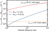Fig. 14 Volatile enrichment timescale as a function of orbital distance. In the inner disk (<10 au), volatiles sublimating at a depth of approximately 0.1 RB (red line) are efficiently lost through convective mixing (τrec,con; dashed orange line). In the colder outer disk, volatiles sublimate at greater depths in the envelope: at a depth of 0.01 RB (blue curve) volatiles are typically deposited in the radiative zone of the envelope where recycling timescales are long (τrec,ad; dashed light blue line), preventing material exchange. The dashed light blue line is truncated at 5 au, since we expect that the envelopes are prone to becoming fully convective in the inner disk (Fig. 13).

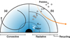Fig. 15 Schematic illustration of an envelope with a convective envelope (side a) and an envelope with a shielding radiative layer and an outer recycling layer (side b).

5.6 Impact of envelope dynamics on planetary growth

Envelope dynamics impact pebble accretion rates. Recycling flows can suppress the accretion of small pebbles by deflecting them away from the planetary core (Kuwahara & Kurokawa 2020a,b; Okamura & Kobayashi 2021). Convective motions can further disrupt pebble trajectories (Popovas et al. 2018, 2019).

Although not modeled in this study, pebbles entering the envelope are expected to undergo thermal ablation (Alibert 2017; Brouwers et al. 2018). When gas recycling is efficient, vaporized material is likely to escape the envelope, limiting core growth (Alibert 2017). However, when radiative layers are more stable and recycling is less efficient, metal-rich material can be retained, possibly contributing to envelope enrichment (Brouwers et al. 2018; Brouwers & Ormel 2020; Ormel et al. 2021). Moreover, processes such as pebble erosion, fragmentation, and growth can significantly alter pebble transport and retention within the envelope (Ali-Dib & Thompson 2020; Johansen & Nordlund 2020). Future studies should aim to couple hydrodynamic simulations with detailed pebble dynamics to better understand the coevolution of pebble and envelope during planet formation.

5.7 Sustainability of dynamical states in envelopes

The dynamical state of an envelope varies significantly depending on the cooling efficiency of the gas. If dust is the dominant source of opacity within the envelope, this leads to a fundamental question: can the convective or radiative layer continue to be sustained?

Let us consider an initially fully convective envelope. In this case, the entire envelope is expected to be recycled in a short timescale. Since small dust particles, which contribute to large opacity, are tightly coupled to the gas, convection can reduce the abundance of small dust within the envelope, leading to a decrease in opacity. As a result, radiative cooling can become more effective, suppressing convection. Meanwhile the planet continues to accrete pebbles. Through processes such as pebble fragmentation within the envelope, the abundance of small dust grains could be enhanced, thereby increasing the opacity and reinitiating convection. The dust supply rate into the envelope depends on factors such as dust size and the 3D structure of the recycling layer. Ultimately, future multi-fluid (gas and dust) 3D simulations coupled with dust growth and fragmentation are needed to understand the complete evolution and structure of the envelope in detail.

6 Conclusions

We conducted a suite of 3D hydrodynamical simulations to characterize the structure and dynamics of planetary envelopes under a wide range of radiative cooling and accretion heating conditions. By varying the dimensionless cooling timescale (β), we identified three distinct envelope regimes: fast cooling (β ≲ 1), intermediate cooling (1 ≲ β ≲ 300), and slow cooling (β ≳ 1000). Each regime exhibits a characteristic envelope structure. In the fast cooling regime, the envelope is nearly isothermal, featuring an inner radiative layer largely shielded from disk gas recycling. In the intermediate cooling regime, the envelope develops a three-layer structure comprising an inner convective layer, a middle radiative layer, and an outer recycling layer. In the slow cooling regime, the entire envelope is fully convective, which allows efficient recycling throughout the envelope.

We developed analytic models for convective and radiative transport timescales that successfully reproduce the tracer particle evolution in each cooling regime. These models demonstrate that fully convective envelopes exchange material within approximately 3 orbits, while envelopes with radiative layers exchange material on longer timescales exceeding 10⁴ orbits.

By comparing the volatile enrichment timescale (τ_vol) with the material exchange timescale (τ_rec), we found that envelopes formed in the inner disk (≲ 1 au) are prone to becoming fully convective. In such envelopes, the volatile enrichment timescale (τ_vol) exceeds the material exchange timescale (τ_rec), implying that these planets will be volatile-poor. Conversely, in the outer disk (≳ 10 au), radiative layers are more likely to develop at r ≲ 0.4−0.6 R_B, for which τ_vol<τ_rec, enabling the accumulation of sublimated volatiles in the envelope’s interior. This spatial variation implies a potential dichotomy in planetary compositions depending on where in the disk a planet forms.

To conclude, our work highlights the need to consider both envelope gas dynamics and thermodynamics when assessing planetary growth and composition. We hope this motivates the development of future models that incorporate dust evolution, radiative transfer, and multi-fluid dynamics to better understand the coevolution of gas, solids, and volatiles during planet formation.

Acknowledgements

We would like to thank an anonymous referee for the positive and encouraging report, that has improved the quality of this manuscript. We thank the Athena++ developers. The Tycho supercomputer hosted at the SCIENCE HPC center at the University of Copenhagen was used for supporting this work. M.L. acknowledge the ERC starting grant 101041466-EXODOSS. Helpful discussions with Ziyan Xu.

References

Appendix A Convergence tests

In this section we investigate how the simulation results depend on numerical settings: the resolution in the radial direction, N_r, the size of the inner boundary, r_in, the spatial reconstruction method (denoted as xoder=2 or 3), and the form of the gravitational potential. Throughout the main text, we adopt N_r=256, r_in=10 R_p, xorder=2, and the gravitational potential defined as Φ_p=−G M_p/r × f_sm × f_inj (Eq. 5).

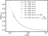Fig. A.1 Shell-averaged temperature for different radial resolutions, inner boundaries, spatial reconstruction methods, and potential formulas. We set m=0.1 and β=103.

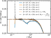Fig. A.2 Shell-averaged temperature gradient for different β, inner boundaries, spatial reconstruction methods, and potential formulas. We set m=0.1 and Nr=256.

Figure A.1 shows the shell-averaged temperature profiles for a fully convective envelope (with m=0.1 and β=10³). All curves are in excellent agreement, except for the one using a gravitational potential of the form ${\Phi }_{\mathrm{p}}=-G{M}_{\mathrm{p}}/\sqrt{r^2+r_{\mathrm{sm}}^2}$ (the dashed-dotted black line). Zhu et al. (2021) argued that high spatial resolution is required to model the envelope accurately, resolving the Bondi radius with approximately 76 grids in the radial direction. In our numerical setup, this corresponds to N_r > 160. As shown in Fig. A.1, all runs with N_r = 168, 196, and 256 yield nearly identical results, confirming sufficient resolution.

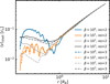Fig. A.3 Shell-averaged mean flow speed for different β and spatial reconstruction methods. We set m = 0.1, Nr = 256, rin = 10 Rp, and Φp=−G Mp/r × fsm × finj.

Using the potential of ${\Phi }_{\mathrm{p}}=-G{M}_{\mathrm{p}}/\sqrt{r^2+r_{\mathrm{sm}}^2}$ causes nonzero gravitational force at the inner boundary, leading to a temperature jump at r_in, as well as a sharp spike in the temperature gradient (Fig. A.2). A similar temperature gradient jump is observed when adopting xorder=3. Additionally, although higher-order piecewise parabolic method method (xorder=3) is generally considered more suitable for maintaining hydrostatic balance than lower-order PLM method (xorder=2; Stone et al. 2020; Zhu et al. 2021), shell-averaged quantities exhibit fluctuations in the xorder=3 case not present in the xorder=2 case. The origin of the fluctuation is unclear, but it is certainly not caused by the averaging method. Nevertheless, across a wide radial range excluding the inner boundary, the results for xorder=2 and 3 agree well despite the fluctuations (Figs. A.2 and A.3). Therefore, we adopted xorder=2 as the default spatial reconstruction method in this study.

Appendix B Fitting formulae for ${\mathit{r}}_{\mathbf{R}\mathbf{C}\mathbf{B}}^{\mathbf{f}\mathbf{i}\mathbf{t}}$ and ${\mathit{r}}_{\mathbf{R}\mathbf{R}\mathbf{B}}^{\text{fit}}$

We introduced the fitting formulae for the boundary between the radiative and convective (RCB) layers, and the recycling and radiative (RRB) layers. We used the scipy.optimize.curve_fit library of python to constrain the fitting coefficients. We assumed that the numerical results, $r_{\text{RCB}}^{\text{num}}$ (Eq. 23), can be fitted by the following sigmoid curve: $$r_{\mathrm{RCB}}^{\mathrm{fit}}=r_{\mathrm{in}}+a_{\mathrm{fit}}[1+tanh\left\{b_{\mathrm{fit}}({log}_{10}\beta -c_{\mathrm{fit}})\right\}](\beta >1).$$(B.1) Here a_fit=0.042, b_fit=5.26, and c_fit=2.09 are the fitting coefficients. Equation B.1 approaches $r_{\mathrm{RCB}}^{\mathrm{fit}}\to r_{\mathrm{in}}$, due to the limitation of the computational domain. We then assumed that the numerically calculated RRB can be fitted by $$r_{\mathrm{RRB}}^{\mathrm{fit}}=\{\begin{array}{c}min(R_{\mathrm{atm}}^{\mathrm{KK}24},R_{\mathrm{atm}}^{\mathrm{KK}24}\times {\beta }^{d_{\mathrm{fit}}})(\beta \le 1),\hfill \\ R_{\mathrm{atm}}^{\mathrm{KK}24}(1+\frac{r_{\mathrm{in}}}{R_{\mathrm{B}}}-\frac{r_{\mathrm{RCB}}^{\mathrm{fit}}}{R_{\mathrm{B}}})(\beta >1),\hfill \end{array}$$(B.2) with d_fit=0.22 being the fitting coefficient and $R_{\mathrm{atm}}^{\mathrm{KK}24}$ determined as in Eq. 30.

Appendix C Characteristic convective flow speed

Here we consider the energy is transported by convection, deriving the characteristic convective flow speed based on the mixing length theory (e.g., Kippenhahn et al. 1990; Ali-Dib & Thompson 2020). The convective energy flux is given by $$F_{\mathrm{con}}=\rho c_{\mathrm{P}}{v}_{\mathrm{con}}\Delta T,$$(C.1) where Δ T is the temperature difference between a convective element and the surrounding. Then the luminosity is given by $$L_{\mathrm{acc}}=4\pi r^2{F}_{\mathrm{con}}.$$(C.2)

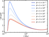Fig. C.1 Shell-averaged pressure gradient for different β. We set m= 0.1 and Ṁ=10 M⊕/Myr.

The convective element is subject to a buoyancy force per unit mass, $$F_{\mathrm{b}}=-\frac{\Delta \rho }{\rho }\left(\frac{G{M}_{\mathrm{P}}}{r^2}\right)\approx -\frac{\Delta T}{T}\left(\frac{1}{\rho }\frac{\partial p}{\partial r}\right),$$(C.3) where Δρ is the density difference between the convective element and the surrounding. In the above equation, we use a hydrostatic equation and assumed a pressure equilibrium. We considered that the convective element moves by a certain distance from 0 to l_m due to the work done by the buoyancy force. Then the average length can be set to l_m/2. We assumed that the half of the work by the buoyancy force is equal to the kinetic energy, $$F_{\mathrm{b}}\times \frac{l_{\mathrm{m}}}{2}\times \frac{1}{2}=\frac{v_{\text{con}}^2}{2}.$$(C.4) From Eqs. (C.1)–(C.4) together with the Meyer’s relation, we have $$v_{\mathrm{con}}={\left[\frac{1}{8\pi r^2}\frac{\gamma -1}{\gamma }\frac{1}{R_{\mathrm{g}}T}(-\frac{1}{\rho }\frac{\partial p}{\partial r})\frac{l_{\mathrm{m}}{L}_{\mathrm{acc}}}{\rho }\right]}^{1/3},$$(C.5) $$={\left[\frac{1}{8\pi r^3}\frac{\gamma -1}{\gamma }(-\frac{\partial lnp}{\partial lnr})\frac{l_{\mathrm{m}}{L}_{\mathrm{acc}}}{\rho }\right]}^{1/3},$$(C.6) $$\approx {\left(\frac{1}{8\pi r^3}\frac{\gamma -1}{\gamma }\frac{l_{\mathrm{m}}{L}_{\mathrm{acc}}}{\rho }\right)}^{1/3},$$(C.7) where R_g is the gas constant. In the above equation, we assumed p=ρ R_g T and −∂ ln p/∂ ln r ≈ O(1) (Fig. C.1).

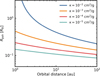Fig. D.1 Photospheric radius for different opacities as a function of the orbital distance.

Appendix D Photospheric radius

The optical depth of the envelope depends on the opacity, and in particular, the deep part of the envelope, inside the photosphere, is always optically thick (Rafikov 2006). The radius of the photosphere is given by $$R_{\mathrm{psh}}\approx \frac{R_{\mathrm{B}}}{ln({\lambda }_{\mathrm{mfp}}/R_{\mathrm{B}})},$$(D.1) where λ_mfp=1 /(κ ρ₀) is the mean free path. Equation D.1 is plotted in Fig. D.1 for different opacities. Our simulations are conducted over a domain that extends beyond r ≳ 0.1 R_B, and therefore, the assumption of optically thin conditions is valid when κ ≲ 10⁻⁵−10⁻⁴ cm²/g or at distances outside of ≳ 10 au.

Appendix E Cooling time estimation

The cooling time of the background gas is determined by two components (Miranda & Rafikov 2020; Ziampras et al. 2023): surface cooling (radiative cooling from the disk surface) and in-plane cooling (radial thermal diffusion through the disk midplane). This is given by (Ziampras et al. 2023) $${\beta }_{\text{surf}}\equiv \frac{{\Sigma }_0{c}_{\mathrm{V}}}{2{\sigma }_{\mathrm{SB}}{T}_0^3}{\tau }_{\text{eff}}\Omega ,{\tau }_{\text{eff}}=\frac{3\tau }{8}+\frac{\sqrt{3}}{4}+\frac{1}{4\tau },\tau =\frac{\kappa {\Sigma }_0}{2},$$(E.1) $${\beta }_{\mathrm{mid}}\equiv \frac{3\kappa {\rho }_0{c}_{\mathrm{V}}}{16{\sigma }_{\mathrm{SB}}{T}_0^3}(H^2+\frac{l_{\mathrm{rad}}^2}{3})\Omega ,l_{\mathrm{rad}}=\frac{1}{\kappa {\rho }_0},$$(E.2) $${\beta }_{\mathrm{disk}}\equiv \frac{{\beta }_{\mathrm{surf}}}{1+{\beta }_{\mathrm{surf}}/{\beta }_{\mathrm{mid}}}.$$(E.3) Here Σ₀ is the gas surface density, T₀ is the midplane temperature, ${\rho }_0={\Sigma }_0/\left(\sqrt{2\pi }H\right)$ is the gas density, c_V=k_B/(μm_H(γ−1)) is the specific heat capacity, κ is the opacity, and σ_SB is the Stefan-Boltzmann constant. Equation E.3 accounts for both optically thick and optically thin regimes.

We considered a two-layer envelope model (Rafikov 2006; Piso & Youdin 2014), assuming the envelope consists of an inner convective layer and an outer radiative layer. The cooling time, namely the time it takes to cool the envelope until the RCB reaches a given pressure depth, is then computed as the ratio of the total energy contained between the core surface and the RCB to the luminosity emerging from the RCB (Piso & Youdin 2014): $${\beta }_{\mathrm{RCB}}\approx 4\pi \frac{p_{\mathrm{RCB}}}{L_{\mathrm{RCB}}\sqrt{R_{\mathrm{p}}}}{\left(\frac{{\nabla }_{\mathrm{ad}}}{\chi }{R}_{\mathrm{B}}\right)}^{1/{\nabla }_{\mathrm{ad}}}\Omega .$$(E.4) Here $$p_{\text{RCB}}=\psi p_0{e}^{R_{\mathrm{B}}/R_{\text{RCB}}},$$(E.5) $$L_{\text{RCB}}\approx L_0\frac{p_0}{p_{\text{RCB}}},L_0=\frac{64\pi G{M}_{\mathrm{p}}{\sigma }_{\mathrm{SB}}{T}_0^4}{3\kappa p_0}{\nabla }_{\text{ad}}{\chi }^4$$(E.6) are the pressure at the RCB ; p₀ is the pressure at the midplane, and the emergent luminosity from the RCB, with ψ=0.556 and χ=1.53 being the constants (Piso & Youdin 2014). Here we adopted a conservative approach to maintaining consistency with the two-layer envelope model in Piso & Youdin (2014). However, we confirmed that using L_acc in Eq. E.4 instead of L_RCB has little impact on the following results.

We defined the envelope cooling time as $${\beta }_{\text{env}}=max({\beta }_{\text{disk}},{\beta }_{\text{RCB}}),$$(E.7) For a fixed planetary mass, orbital distance and a specific disk model, β_env is determined as a function of opacity and the RCB location, as shown in Fig. 13. We used a passively irradiated disk model to compute the physical quantities at the midplane (Oka et al. 2011), $${\Sigma }_0=2.7\times {10}^3\mathrm{g}/{\mathrm{cm}}^2{\left(\frac{a_{\mathrm{p}}}{1\mathrm{au}}\right)}^{\xi },T_0=150\mathrm{K}{\left(\frac{a_{\mathrm{p}}}{1\mathrm{au}}\right)}^{\zeta }.$$(E.8) We chose here a purely irradiated disk with ξ=−15/14 and ζ = −3/7.

All Tables

All Figures

	Fig. 1 Shell-averaged density, temperature, entropy, and temperature gradient (from top to bottom) for different β values. We set m=0.1 and Ṁ=10 M⊕/Myr. All panels are the snapshots at the end of the calculation, t=50. The dashed and dotted curves in panels a–c are the analytic models given by Eqs. (18), (25), and (26). The horizontal dashed line in panel d is the adiabatic gradient, Eq. (20).
In the text

	Fig. 2 Radial velocity of the gas as a function of cooling time (β). We set m=0.1 and Ṁ=10 M⊕/Myr. All panels are snapshots at the end of the calculation, t=50. The dashed circle denotes the Bondi radius. Top: midplane slices, with streamlines shown in panel a. Bottom: vertical slices where the velocity is hemispherically averaged in the azimuthal direction, φ ∈[−π/2, π/2].
In the text

	Fig. 3 Hemispherically and time-averaged density and velocity vector on the vertical slice. We set m=0.1. The physical quantities are averaged over the azimuth and the time, φ ∈[−π/2, π/2] and t ∈[40, 50]. The dashed white circle in the top panels is the Bondi radius of the planet.
In the text

	Fig. 4 Boundary between the recycling and radiative layers (orange) and the radiative and convective layers (blue), as a function of cooling time (β). The squares and circles are the numerical results, obtained for m=0.1 and Ṁ=10 M⊕/Myr. The dashed lines are the fitting formulae (Appendix B). The hatched region is not probed by our simulations.
In the text

	Fig. 5 Shell-averaged mean speed for β=10−2−101. We set m=0.1 and Ṁ=10 M⊕/Myr. This figure shows the state at the end of the simulation, t=50. The radiative and recycling layers are qualitatively indicated. The horizontal dotted lines correspond to Eq. (22) with r=0.3 RB and r=0.8 RB. The dashed-dotted gray curve represents Eq. (22).
In the text

	Fig. 6 Shell-averaged radial velocity (solid lines) and azimuthal velocity (dashed lines), for different β. Negative components are omitted. We set m=0.1 and Ṁ=10 M⊕/Myr. The dotted gray line represents the Keplerian velocity around the core.
In the text

	Fig. 7 Same as Fig. 5 but for β=102 and 103. The convective, radiative, and recycling layers are qualitatively indicated. The dashed red and yellow curves show Eq. (24), under the assumptions of fully and partially convective envelopes with lm=RB and lm=0.2 RB, respectively.
In the text

Fig. 8 Shell-averaged temperature gradient and mean velocity for different β values and accretion luminosities. All panels are the states at the end of the calculation, t=50. The dashed, solid, and dotted gray curves in panel b are given by Eq. (24) with an assumption of fully convective envelopes (lm=RB). Thus, these gray lines should be compared with the red lines. The dashed-dotted gray curve is given by Eq. (22).

In the text

	Fig. 9 Shell-averaged temperature gradient for different planetary masses and β values. We set Ṁ=10 M⊕/Myr. All panels are the snapshots at the end of the calculation, t=50. The horizontal dashed line is the adiabatic gradient, Eq. (20).
In the text

	Fig. 10 Tracer concentration at the midplane. We set m=0.1. Different rows correspond to different β values (β=100, 102., and 103, from top to bottom). Different columns correspond to different times (t=15, 20, 25, 30, and 50 in code units, from left to right).
In the text

	Fig. 11 Tracer concentration in the x-z plane at the end of the calculation (t=50 in code units), after a hemispherical average along the azimuthal direction.
In the text

Fig. 12 Time evolution of the shell-averaged tracer concentration for β=100 (panel a), 102 (panel b), and 103 (panel c). Different colors correspond to different shell radii. The orange lines are given by Eq. (28). In panel b we set lm=0.2 RB (partially convective) and plot the decay rate at r=0.4 RB (the solid line), r=0.6 RB (the dotted line), and r=0.8 RB (the dashed line), respectively. In panel c, we set lm=RB (fully convective).

In the text

	Fig. 13 Analytic estimate of the envelope’s cooling time as a function of the opacity and the RCB location. Different panels correspond to different orbital locations of the Earth-mass planet.
In the text

Fig. 14 Volatile enrichment timescale as a function of orbital distance. In the inner disk (<10 au), volatiles sublimating at a depth of approximately 0.1 RB (red line) are efficiently lost through convective mixing (τrec,con; dashed orange line). In the colder outer disk, volatiles sublimate at greater depths in the envelope: at a depth of 0.01 RB (blue curve) volatiles are typically deposited in the radiative zone of the envelope where recycling timescales are long (τrec,ad; dashed light blue line), preventing material exchange. The dashed light blue line is truncated at 5 au, since we expect that the envelopes are prone to becoming fully convective in the inner disk (Fig. 13).

In the text

	Fig. 15 Schematic illustration of an envelope with a convective envelope (side a) and an envelope with a shielding radiative layer and an outer recycling layer (side b).
In the text

	Fig. A.1 Shell-averaged temperature for different radial resolutions, inner boundaries, spatial reconstruction methods, and potential formulas. We set m=0.1 and β=103.
In the text

	Fig. A.2 Shell-averaged temperature gradient for different β, inner boundaries, spatial reconstruction methods, and potential formulas. We set m=0.1 and Nr=256.
In the text

	Fig. A.3 Shell-averaged mean flow speed for different β and spatial reconstruction methods. We set m = 0.1, Nr = 256, rin = 10 Rp, and Φp=−G Mp/r × fsm × finj.
In the text

	Fig. C.1 Shell-averaged pressure gradient for different β. We set m= 0.1 and Ṁ=10 M⊕/Myr.
In the text

	Fig. D.1 Photospheric radius for different opacities as a function of the orbital distance.
In the text

References

- Ali-Dib, M., & Thompson, C., 2020, ApJ, 900, 96 [NASA ADS] [CrossRef] [Google Scholar]
- Alibert, Y., 2017, A&A, 606, A69 [NASA ADS] [CrossRef] [EDP Sciences] [Google Scholar]
- Bailey, A. P., & Zhu, Z., 2024, MNRAS, 534, 2953 [Google Scholar]
- Béthune, W., & Rafikov, R. R., 2019, MNRAS, 488, 2365 [Google Scholar]
- Brouwers, M., & Ormel, C., 2020, A&A, 634, A15 [NASA ADS] [CrossRef] [EDP Sciences] [Google Scholar]
- Brouwers, M., Vazan, A., & Ormel, C., 2018, A&A, 611, A65 [NASA ADS] [CrossRef] [EDP Sciences] [Google Scholar]
- Chrenko, O., & Lambrechts, M., 2019, A&A, 626, A109 [NASA ADS] [CrossRef] [EDP Sciences] [Google Scholar]
- Cimerman, N. P., Kuiper, R., & Ormel, C. W., 2017, MNRAS, 471, 4662 [Google Scholar]
- Fung, J., Artymowicz, P., & Wu, Y., 2015, ApJ, 811, 101 [Google Scholar]
- Fung, J., Zhu, Z., & Chiang, E., 2019, ApJ, 887, 152 [NASA ADS] [CrossRef] [Google Scholar]
- Gammie, C. F., 2001, ApJ, 553, 174 [Google Scholar]
- Ikoma, M., Nakazawa, K., & Emori, H., 2000, ApJ, 537, 1013 [NASA ADS] [CrossRef] [Google Scholar]
- Johansen, A., & Nordlund, Å. 2020, ApJ, 903, 102 [NASA ADS] [CrossRef] [Google Scholar]
- Johansen, A., Ronnet, T., Bizzarro, M., et al. 2021, Sci. Adv., 7, eabc0444 [Google Scholar]
- Kippenhahn, R., Weigert, A., & Weiss, A., 1990, Stellar Structure and Evolution (Berlin: Springer), 192 [Google Scholar]
- Krapp, L., Kratter, K. M., & Youdin, A. N., 2022, ApJ, 928, 156 [NASA ADS] [CrossRef] [Google Scholar]
- Kurokawa, H., & Tanigawa, T., 2018, MNRAS, 479, 635 [Google Scholar]
- Kuwahara, A., & Kurokawa, H. 2020a, A&A, 633, A81 [NASA ADS] [CrossRef] [EDP Sciences] [Google Scholar]
- Kuwahara, A., & Kurokawa, H. 2020b, A&A, 643, A21 [NASA ADS] [CrossRef] [EDP Sciences] [Google Scholar]
- Kuwahara, A., & Kurokawa, H., 2024, A&A, 682, A14 [NASA ADS] [CrossRef] [EDP Sciences] [Google Scholar]
- Kuwahara, A., Kurokawa, H., & Ida, S., 2019, A&A, 623, A179 [NASA ADS] [CrossRef] [EDP Sciences] [Google Scholar]
- Lambrechts, M., & Johansen, A., 2012, A&A, 544, A32 [NASA ADS] [CrossRef] [EDP Sciences] [Google Scholar]
- Lambrechts, M., & Lega, E., 2017, A&A, 606, A146 [NASA ADS] [CrossRef] [EDP Sciences] [Google Scholar]
- Lambrechts, M., Johansen, A., & Morbidelli, A., 2014, A&A, 572, A35 [NASA ADS] [CrossRef] [EDP Sciences] [Google Scholar]
- Miranda, R., & Rafikov, R. R., 2020, ApJ, 904, 121 [NASA ADS] [CrossRef] [Google Scholar]
- Mizuno, H., 1980, Prog. Theor. Phys., 64, 544 [Google Scholar]
- Moldenhauer, T., Kuiper, R., Kley, W., & Ormel, C., 2021, A&A, 646, L11 [NASA ADS] [CrossRef] [EDP Sciences] [Google Scholar]
- Moldenhauer, T., Kuiper, R., Kley, W., & Ormel, C., 2022, A&A, 661, A142 [NASA ADS] [CrossRef] [EDP Sciences] [Google Scholar]
- Mordasini, C., 2014, A&A, 572, A118 [NASA ADS] [CrossRef] [EDP Sciences] [Google Scholar]
- Oka, A., Nakamoto, T., & Ida, S., 2011, ApJ, 738, 141 [Google Scholar]
- Okamura, T., & Kobayashi, H., 2021, ApJ, 916, 109 [NASA ADS] [CrossRef] [Google Scholar]
- Ormel, C. W., 2014, ApJ, 789, L18 [Google Scholar]
- Ormel, C. W., & Klahr, H. H., 2010, A&A, 520, A43 [NASA ADS] [CrossRef] [EDP Sciences] [Google Scholar]
- Ormel, C. W., Kuiper, R., & Shi, J.-M., 2015a, MNRAS, 446, 1026 [NASA ADS] [CrossRef] [Google Scholar]
- Ormel, C. W., Shi, J.-M., & Kuiper, R., 2015b, MNRAS, 447, 3512 [Google Scholar]
- Ormel, C. W., Vazan, A., & Brouwers, M. G., 2021, A&A, 647, A175 [NASA ADS] [CrossRef] [EDP Sciences] [Google Scholar]
- Piso, A.-M. A., & Youdin, A. N., 2014, ApJ, 786, 21 [NASA ADS] [CrossRef] [Google Scholar]
- Pollack, J. B., Hubickyj, O., Bodenheimer, P., et al. 1996, Icarus, 124, 62 [NASA ADS] [CrossRef] [Google Scholar]
- Popovas, A., Nordlund, Å., Ramsey, J. P., & Ormel, C. W. 2018, MNRAS, 479, 5136 [Google Scholar]
- Popovas, A., Nordlund, Å., & Ramsey, J. P. 2019, MNRAS, 482, L107 [NASA ADS] [CrossRef] [Google Scholar]
- Rafikov, R. R., 2006, ApJ, 648, 666 [Google Scholar]
- Stone, J. M., Tomida, K., White, C. J., & Felker, K. G., 2020, ApJS, 249, 4 [NASA ADS] [CrossRef] [Google Scholar]
- Wang, Y., Ormel, C. W., Huang, P., & Kuiper, R., 2023, MNRAS, 523, 6186 [NASA ADS] [CrossRef] [Google Scholar]
- Zhu, Z., Jiang, Y.-F., Baehr, H., et al. 2021, MNRAS, 508, 453 [NASA ADS] [CrossRef] [Google Scholar]
- Ziampras, A., Nelson, R. P., & Rafikov, R. R., 2023, MNRAS, 524, 3930 [NASA ADS] [CrossRef] [Google Scholar]
We used the public version of Athena++ (ver 24.0), which is available at https://github.com/PrincetonUniversity/athena