| Issue |
A&A
Volume 707, March 2026
|
|
|---|---|---|
| Article Number | A237 | |
| Number of page(s) | 16 | |
| Section | The Sun and the Heliosphere | |
| DOI | https://doi.org/10.1051/0004-6361/202557855 | |
| Published online | 09 March 2026 | |
DeepFilter: A machine learning technique for removing the hot AIA 304 Å channel component for the analysis of coronal rain
1
Northumbria University, Ellison Place Newcastle upon Tyne, United Kingdom
2
Astronomical Institute of the University of Bern Sidlerstrasse 5 3012 Bern, Switzerland
3
University of Applied Sciences and Arts Northwestern Switzerland Bahnhofstrasse 6 CH-5210 Windisch, Switzerland
★ Corresponding author: This email address is being protected from spambots. You need JavaScript enabled to view it.
Received:
27
October
2025
Accepted:
9
January
2026
Abstract
The Atmosphere Imaging Assembly (AIA) 304 Å channel aboard the Solar Dynamic Observatory offers an unparalleled full-disk view of cool material at T ≈ 105 K emitted by the He II 304 Å spectral line. This opens the possibility for the in-depth and widespread analysis of the formation and evolution of small cool structures seen in the solar atmosphere. Of particular interest is the phenomenon of coronal rain, which has been linked to the overarching heating and cooling cycles of the solar corona. However, within the channel’s passband, hot diffuse emission from several ions is also included, leading to comparable intensity levels to the cool emission, particularly off-limb. This makes it very difficult to disentangle cool coronal rain from this hotter material. In this paper a novel morphological approach to separating these components called DeepFilter is investigated. This approach utilises a generative machine learning algorithm that can learn how to convert the AIA 304 Å images into the style of images obtained with the Interface Region Imaging Spectrograph (IRIS) 1400 Å, which has a similar temperature formation peak as for He II 304 Å but lacks this hot-component contamination. We find that the method produces good results, showing a clear reduction in the amount of hot-component material present in the final images while preserving the majority of the underlying cool structures. DeepFilter is compared to the recent physics-based RFit algorithm and is found to produce comparable results. Although the DeepFilter method is shown to perform worse at removing hot emission and material far from the limb, it performs comparably on other data – with the advantage of being far less data intensive – which makes it more effective for large-scale statistical analysis.
Key words: line: profiles / methods: data analysis / methods: statistical / techniques: image processing / Sun: corona
© The Authors 2026
 Open Access article, published by EDP Sciences, under the terms of the Creative Commons Attribution License (https://creativecommons.org/licenses/by/4.0), which permits unrestricted use, distribution, and reproduction in any medium, provided the original work is properly cited.
This article is published in open access under the Subscribe to Open model. This email address is being protected from spambots. You need JavaScript enabled to view it. to support open access publication.
1. Introduction
The phenomenon known as coronal rain is a catastrophically cooling event consisting of cool, dense, partially ionised plasma that appears in clumps (also known as condensations), over the space of a few minutes in magnetic coronal loops. These clumps of plasma then fall along these loops at a broad distribution of spatial velocities around 80 km s−1 (Antolin et al. 2012; Kleint et al. 2014). The primary properties of the phenomena are their higher density and lower temperature when compared to the surrounding corona. The rain is visible in spectral lines common to the chromosphere and transition region due to their temperatures of a few 103 K to several 105 K (Antolin 2019). This broad temperature range of the composite plasma leads to co-spatial multi-wavelength emission from the rain.
To understand the importance of the rain, it is first crucial to understand that the coronal loops are constantly subject to heating and cooling processes (Klimchuk 2006). The current working hypothesis for the formation mechanism of coronal rain is that it is produced as a by-product of this coronal heating in the solar atmosphere, which causes a cyclical feedback process known as the thermal non-equilibrium (TNE) cycle. This cycle can be broadly described by the following mechanisms:
1.1. Footpoint heating.
The magnetic flux tube is heated by quasi-steady heating of a yet unknown nature at the footpoints of the coronal loop, occurring with a frequency higher than that set by the radiative cooling time. Thermal conduction then distributes energy along the flux tube, rapidly heating it up, balancing against radiation. The majority of the energy is transferred to the transition region and upper chromosphere. Here it is radiated away, additionally heating up the plasma.
1.2. Chromospheric evaporation.
The heated plasma is ablated and fills the coronal loop due to the increase in pressure (the ‘evaporation’ term does not indicate a phase transition in this context). The temperature increases followed by density as the material reaches the corona. The plasma becomes over-dense, relative to thermal equilibrium, and begins to radiate more than the thermal conductive heating influx.
1.3. Condensation.
As the density builds in the corona, the radiative losses overcome the heating. As a result, the plasma begins to cool down. This cooling is accelerated because the radiative loss rate increases for lower temperatures in the range between ≈105 K and ≈106 K. During this runaway cooling process, thermal instability is triggered, further accelerating cooling to transition region or chromospheric temperatures. The exact route to this thermal instability is still a matter of considerable debate: whether it is an isobaric or isochoric process (Claes & Keppens 2019; Keppens et al. 2025), or involves no thermal mode at all (Klimchuk & Luna 2019; Waters & Stricklan 2025). Regardless, this process is accompanied by a local loss of pressure, which produces plasma accumulation, that is 2 orders of magnitude denser than the surroundings (Antolin et al. 2015). These condensations fall back down towards the chromosphere at the feet of the loop under gravity, constrained by gas pressure, evacuating the flux tube. It is these falling condensations, which are known as coronal rain. It is worth noting that condensations can also occur in coronal structures with magnetic dips such as flux ropes, leading to the generation of prominences (Xia et al. 2011, 2014; Yoshihisa et al. 2024). If heating remains stable, the cycle restarts in the newly evacuated magnetic flux tube leading to TNE cycles with specific periods (Antiochos et al. 1999; Karpen et al. 2001; Antolin et al. 2010; Froment et al. 2017; Klimchuk & Luna 2019; Antolin & Froment 2022).
It is the link to dynamic heating-cooling mechanisms such as TNE that leads to the current interest in this phenomenon and how it can relate to and elucidate the enigmatic heating of the corona. It might seem counter-intuitive to track coronal rain, in the context of solving the coronal heating problem, as it results from a cooling effect. However, if coronal rain formation is driven by the aforesaid TNE cycle the main drive to study rain becomes its ability to differentiate the type of heating taking place in the coronal loop footpoints. It has been argued that coronal loops lacking any rain are heated via mechanisms that exhibit uniform heating of the loop – such as non-linear Alfvén waves dissipating through shocks (Antolin et al. 2010) – which inhibits the TNE cycle. Conversely, loops demonstrating coronal rain may be heated by spatially and temporally constrained footpoint heating – for example that resulting from slow magnetic stress from convective motions (Lionello et al. 2013). Although consensus on the heating mechanism driving coronal rain has yet to be reached, papers shows that DC-type heating (such as slow magnetic stress from convective motions) events can cause coronal rain formation (Kohutova et al. 2020). Nevertheless if the amount of coronal rain can be accurately quantified and its distribution within the Sun’s atmosphere understood, it will allow for better determination of footpoint heating occurrence – and possibly its origin.
A full quantitative analysis to date has not been carried out on the phenomenon for a number of different reasons. Chief among these is the highly localised, sparse but pervasive – and dynamic – nature of coronal rain, which makes it extremely difficult to accurately count events at any given time across the solar atmosphere or quantify the associated plasma. The development of a methodology to do just that is further hampered by the observational data currently available. To illustrate this point, for the observation of coronal rain there are currently two primary observational instruments used, namely the Atmospheric Imaging Assembly (AIA) (Lemen et al. 2012) and the Slit-Jaw Imager (SJI) of the Interface Region Imaging Spectrograph (IRIS) (De Pontieu et al. 2014), both seen in Figure 1. Of the two, IRIS has greater spatial resolution ranging between 0.33″ and 0.44″ (compared to AIA’s 1.6″), which, combined with the Slit-Jaw Imagers (SJI) dominated by chromospheric and low transition region emission in the UV (1330 Å, 1400 Å and 2796 Å SJI channels), allows the instrument to observe rain in much greater detail and lower temperature ambiguity. The main hold back of the instrument is its small field of view (FOV) of 175″ × 175″, which limits detection. Alternatively, SDO/AIA, with its full-disk FOV and 12 s cadence is best able to capture coronal rain in the 304 Å channel, which is dominated by He II emission at 304.02 Å forming at ≈105 K. However, the AIA 304 Å has a broad effective area that includes emission from hotter ions, which increase temperature ambiguity of the visualised plasma. To illustrate this, Figure 2 shows the temperature response of the AIA 304 Å channel as well as the temperature result of IRIS 1400 Å. From the figure, two clear maxima can be seen for AIA 304 Å: a main peak at T ≈ 105 K corresponding to the He II line, and another significant peak at T ≈ 106.25 K, corresponding primarily to the Si XI 303.32 Å line – though with contributions from many other emissions lines in this hot temperature range (Tousey et al. 1965; Thompson & Brekke 2000). For ease these two contributions seen in the temperature response of AIA 304 Å are referred to as the cool and hot component. For the IRIS 1400 Å temperature response, it is calculated with CHIANTI version 11 (Dufresne et al. 2024), with the ‘advanced model’ option switched on to account for the effects of charge transfer on ionisation and recombination rates. For this calculation, we chose the ‘Fontenla Plage’ model atmosphere (Fontenla et al. 2014) to account for active regions (ARs) and set the number density equal to 109 cm−3. We took the 2021 coronal abundances (sun_coronal_2021_chianti.abund). We also added the continuum and all lines to this calculation. The resulting spectrum was multiplied with the effective area (interpolated to the wavelength array output from the isothermal routine calculation), the ratio of proton density to electron density (calculated with the proton_dens CHIANTI routine for the same temperature range), and the area of the IRIS pixel in radians.
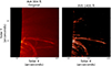 |
Fig. 1. Examples of AIA (left) and IRIS (right) co-aligned images of the same coronal rain event. As can be seen, the AIA contains a much greater amount of diffuse material due to the contribution of the hot component of its temperature response. In contrast, the coronal rain structures in the IRIS image are much more easily differentiated from the surroundings. |
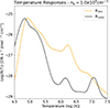 |
Fig. 2. Temperature response functions for the AIA 304 Å and IRIS 1400 Å channels. It is worth noting that the response function was calculated based on the CHIANTI database, which has been known to fail at reproducing the He II intensity peak between 104.8–104.9 K, where the resulting peak is an order of magnitude lower. This is likely due to the effects of non-equilibrium ionisation in tandem with optically thick radiative transfer in the He II line causing these large intensities (Golding et al. 2017). To account for this, the AIA 304 Å response function has been multiplied by an empirical factor of 5 (O’Dwyer et al. 2010). |
Although the contribution from the hot component in AIA 304 Å is an order of magnitude less than that from the cool component, it is crucial to remove this hotter component from the AIA 304 Å images if any precise analysis of coronal rain is to be undertaken using the channel. This occurs because the emission from the hot component can be comparable to that from the cool component when observing off-limb, due to the significantly longer integration paths and the diffuse nature of the hot corona – contrary to the compact emission from the clumpy coronal rain. The impact of this hot component is particularly noticeable when compared with that from the IRIS/SJI channels. Figure 1 shows the same coronal rain event taken by both AIA 304 and IRIS 1400. A clear diffuse region can be seen in the AIA image that is absent from the much higher contrasted IRIS image. As this hot component can appear at similar intensities to the cool component in the images, it becomes incredibly difficult to quantify the amount of cool material in an image without capturing a significant amount of material belonging to this hot component. As such, before any large-scale statistical analysis can take place into the amount and location of rain using AIA 304 Å, this hot component must be first removed.
One current method to disentangle the components of AIA 304 Å, which uses temperature response is known as Response Fit (Antolin et al. 2024), referred to as RFit in this paper. This technique uses all six other EUV channels in the AIA instrument to linearly fit the temperature response profile of the hot AIA 304 component line with the temperature responses of the other EUV channels. Once the relative weights of all the other EUV channels are calculated to approximate the hot-component temperature response, a ‘hot’ image can be generated containing emission exclusively within this hot temperature range (dominated by Si XI 303.32 Å). This can then be subtracted from the original image to produce an image of just the He II line in the AIA image. For this we take the response functions from Solarsoft, obtained with the IDL command aia_get_response(/dn,/temp,/chiantifix,/eve,timedepend_date=date). From this command, the dn keyword means DN units, the temp keyword specifies the temperature response function, the chiantifix keyword applies an empirical correction to the AIA 94 and AIA 131 channels needed to account for emission not included in CHIANTI, and the eve keyword provides good overall agreement with the Extreme Ultraviolet Variability Experiment (EVE) of SDO. Solarsoft calculates these response functions with CHIANTI version 10 (Del Zanna et al. 2021). The primary disadvantage of this is that it requires information from the other AIA EUV channels to generate hot-component-filtered images, which can increase data acquisition complexity of the phenomena and generally slow down analysis.
2. The DeepFilter algorithm
To overcome the problems highlighted by the RFit method of removing the hot component of the AIA 304 Å namely its reliance on many EUV channels, which drastically increases the computational time and data requirements, a new technique based on morphology has been created. This technique does not rely on additional channels in the process and enables the preservation of the image’s intensity values. This novel approach makes use of the fact that coronal rain is captured not only with AIA but also with IRIS as discussed earlier. Although IRIS’ FOV limits the ability to carry out large-scale quantification of coronal rain, it can be used as a machine-learning target training set in a style conversion algorithm that can convert AIA 304 Å with hot-component contaminants into the style of IRIS 1400 Å, which has no such contaminants. In this way, we automatically filter the hot component without the need for supplementary data – hence the name DeepFilter.
2.1. Basic principles
The DeepFilter model has been designed for the express purpose of solving the AIA 304 Å hot-component problem. It is a modified version of the CycleGAN algorithm for unpaired image translation (Zhu et al. 2017). The essential idea of a CycleGAN is that any set of images in a specific style domain can be converted to the style of another set of images. By style we mean the core features – such as shared contrasts, colour schemes, and structures – that allow differentiation of a certain image set from another (e.g. the difference between Van Gogh’s ’Starry night’ and a photo-realistic image of the sky). In this regard an IRIS image of coronal rain’s style will be characterised by high-contrast, fine-stranded structures against a dark background, largely free of the diffuse emission that defines the style of the AIA 304 Å images. Crucially, the algorithm does not require a paired set of images with which to transform. Rather, it learns the inherent features of a style and how to generally map between styles. Finding the correct style transfer then allows individual images to be converted into the target style without the need for a direct counterpart. The reason an unpaired algorithm was used, as opposed to creating and utilising a paired image approach, is that coronal rain structure can be highly variable, and this approach enables the resultant model to translate morphologically dissimilar images, without being over-trained to expect certain morphologies. To carry out the style transfer, there are two crucial concepts to understand: the concept of a generative adversarial network (GAN) and the concept of maintaining cycle consistency. Furthermore, the tertiary concept of identity loss was added and is also discussed.
2.1.1. Generative adversarial networks (GANs)
First introduced a decade ago in 2014 (Goodfellow et al. 2014), a GAN is an image translation deep network built on the idea of two separate component networks in opposition to one another. This competition between the two sides eventually leads to the network as a whole learning the optimal way of translating between styles. The first component network of the algorithm is a network known as a ‘Generator’, and as the name suggests it is the component, which carries out the actual style transfer. It takes as its input the original image to transfer, encodes this down into a feature space consisting of a vector matrix of the features of the image that constitute the style of the image, alters this feature space to fit that of the target domain, then decodes that feature space into a new image with the style of the target domain. On the other side of this adversarial pair is a network known as a ‘Discriminator’, designed to distinguish between an image with the desired style and those without. It can be thought of as a well trained binary classifier. The key to understanding how these two components communicate is the metric of adversarial loss. This loss function measures the similarity between a generated image and that of the target domain. The lower the loss between images the more similar their style. The Generator aims at minimising the loss between the created images and the target domain, while the Discriminator attempts to maximise the loss between the produced images and the target domain. They repeat this until a state known as Nash equilibrium (Zhao et al. 2017) is found. This is the point where the distribution of the Generator converges maximally with the distribution of the training data. Here, the Discriminator shows the greatest confusion as it distinguishes between synthetic and real data in the target domain.
2.1.2. Cycle consistency
The second key concept employed by CycleGANs is cycle consistency: the inherent structure of the original image must remain intact enough to allow the successful reversal of the style transfer. This principle is crucial specifically in domains where structural integrity of the style transfer is necessary. Without a parameter enforcing some maintenance of structure, a simple GAN may learn the easiest way to adapt an image into the style of another by completely altering the mappings of underlying structures. This would not be ideal in any case where the underlying structural elements of an image are required for the resulting style-transferred image.
To maintain cycle consistency alongside training a forward set of generator and discriminator, it is also crucial to train a backward pair. This backward pair is designed to convert images from the original target domain into the style of the original input domain. For example, take an image x1 from style x. Using the forward GAN, this image is translated into the style of domain y to produce image y1. This synthetic image is then sent through the reverse GAN to revert it to style x, to produce image x2. The cycle consistency loss between x1 and x2 can then be calculated to determine the similarity between the original image and the fully cycled image. This creates a cycle loss quantity that the algorithm can work to minimise over the course of training. While a zero value in this loss would imply perfect translation and reconstruction, this cannot be achieved in real-world training scenarios due to complexities such as image variations and network limitations (Wang & Lin 2024).
2.1.3. Identity loss
In addition to the two previous loss functions a further loss term was added to greater constrain the model in regards to maintaining the structural integrity of the images. This third loss function is derived from the fact that if an image belonging to style y is sent through the x-to-y GAN, the resulting image should be near identical to the starting image (Taigman et al. 2017). This identity loss is incorporated into the DeepFilter model by sending an image belonging to style y into the x-to-y GAN. The resulting image y3 can then be compared to the input image to see if any major changes have taken place. Ideally this loss should be small as the algorithm then recognises that no changes are needed. This reduces the chance that the algorithm will learn to add imaginary structures or remove any essential structural elements in the images. Figure 3 gives a simplified diagram of a typical training iteration, which allows us to visualise all three of these losses and the general architecture of the model.
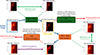 |
Fig. 3. Simplified diagram of a typical training iteration of the DeepFilter algorithm. The diagram is colour-coded to show where each loss function is calculated. Red denotes adversarial loss, purple denotes cycle consistency loss, and green denotes identity loss. The equation where these losses are then used to calculate the total loss during the training is Eq. (5). |
Ultimately, a CycleGAN algorithm’s effectiveness is dictated by the balancing of these key loss functions. On the one hand, the CycleGAN needs to create a synthetic image that minimises the adversarial loss discussed in Section 2.1.1, which promote change in the image; on the other hand, it simultaneously minimises cycle consistency loss and identity loss of the images created, which promote maintaining the original structure. The balance between these two loss functions is highly variable and depends greatly on the domain of the transformation. Our focus in this paper is to use the algorithm to automatically eliminate the diffuse (hot) material from the AIA 304 Å images by commuting the style of the images into IRIS 1400 Å – where such diffuseness is mostly absent – though a diffuse component for SJI 1400 from Fe XXI flare emission exists. For this style transfer purpose, it is imperative that the underlying structure of the coronal rain (or any other cool material seen off-limb in the images) is maintained. Therefore, the balance in this domain transform will be heavily skewed towards prioritising the minimisation of cycle consistency loss and identity loss, even at the possible sacrifice of maintaining a higher adversarial loss.
2.2. Base architecture
2.2.1. Generator
As a starting point, the Generator for the DeepFilter algorithm is based on the Generator used in the original CycleGAN paper by Zhu et al. (2017). The Generator is split into three distinct sections with a visual representation seen in Figure 4. The first of these sections is the encoder stage (also known as the down-sampling stage). This is where an image is supplied to the generator, which encodes this raw data into the more abstract latent feature space. This is a space where the image is now described by specific features and relationships between data points, which the computer can use to define the makeup of the image as a whole. To make this transition from ‘real’ to latent space, a series of convolution layers are carried out that transform the image from a ‘real’ space size of 1 × 512 × 512 to a latent feature space of 256 × 128 × 128. This feature space represents the image by a network 256 filters deep corresponding to the weights of 128 × 128 features. To change the makeup of the image, the algorithm can change the weights between these filters.
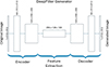 |
Fig. 4. Simplified visual representation of the basic architecture of the CycleGAN Generator. |
The actual interpretive nature of this latent space is a whole active area of study by itself (Liu et al. 2019), and the actual connections and features that the machine learning algorithm determines as important are highly domain specific and often unintuitive. Interestingly, although domain sensitive, it has been previously shown that this latent space and the features generated within are preserved in a large variety of generative architectures (Asperti & Tonelli 2023), implying a natural organisation of a latent space in a domain.
The next stage of the Generator is the extraction of features from this latent space (also known as the transformer stage). This is the stage where the weights between the layers in the feature space are changed to minimise the adversarial loss. In practice, this is achieved by a series of nine residual blocks (see Figure 6), with each block representing a set of 2D convolutional layers, where every two layers are followed by an instance normalisation layer. Each block iteratively learns from the block before to make the optimal change to the network weight.
The final section of the Generator is the decoder (alternatively, up-sampling layer). This carries out the reverse process of the encoder by converting the latent representation back to a ‘real’ image. This is done by a series of deconvolutional layers to turn the 256 × 128 × 128 latent representation into a 1 × 512 × 512 synthetic image. This image can then be sent to the Discriminator for assessment.
2.2.2. Discriminator
The Discriminator utilised for the purpose of this algorithm is a 70 × 70 PatchGAN Discriminator, which has shown previous success in a variety of domains (Isola et al. 2017; Fan et al. 2023). For reference, a simplified visual of the Discriminator is seen in Figure 5. The basic idea of a PatchGAN Discriminator is that an image is encoded into latent feature space by a sequence of convolutional layers, similar to the Generator. However, the image is segmented into a latent array, with each element correspond to overlapping regions of size 70 × 70 pixels from the original image. The Discriminator then acts to classify each of these elements as real or fake relative to the target domain. The final classification is then the average result of all these sub-classifications. In this classification process, the Discriminator is penalised if it incorrectly identifies a synthetic image created by the Generator as real. It does this by attempting to maximise the adversarial loss between itself and the image sent from the generator. An added benefit of the PatchGAN discrimination approach is that it helps retain the structural elements of the images as it only penalises based on local, patch-level style mismatches.
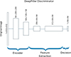 |
Fig. 5. Simplified visual representation of the basic architecture of the base CycleGAN Discriminator. |
2.3. Formalisation of loss
2.3.1. Adversarial loss
If one were to derive the adversarial loss between the mapping function G (which converts an image between domain X and domain Y) and the Y Discriminator DY, the loss function is
![Mathematical equation: $$ \begin{aligned} \begin{aligned} \mathcal{L} _{\mathrm{GAN} }\left(G, D_Y, X, Y\right) =&\mathbb{E} _{y \sim p_{\mathrm{data} }(y)}\left[\log D_Y(y)\right] \\&+\mathbb{E} _{x \sim p_{\mathrm{data} }(x)}\left[\log \left(1-D_Y(G(x))\right]\right., \end{aligned} \end{aligned} $$](/articles/aa/full_html/2026/03/aa57855-25/aa57855-25-eq1.gif) (1)
(1)
where the Generator G attempts to minimise this loss against Discriminator DY, which in turn maximises this loss.
Let us recall that in a CycleGAN there will be a reverse operation as well, which has the same formalisation as above, only using Generator F and Discriminator DX.
2.3.2. Cycle-consistency loss
The forward cycle-consistency loss – between an original image (x1) and its cyclical image (x2) in the X domain (i.e. one sent through a generator to turn into the Y domain, then sent back through a generator, which translates back to the X domain, x1 → G(x)→F(G(x)) = x2 ≈ x1) – is calculated based on the objective function
![Mathematical equation: $$ \begin{aligned} \begin{aligned} \mathcal{L} _{\mathrm{cyc} }(G, F)=\mathbb{E} _{x \sim p_{\mathrm{data} }(x)}\left[\Vert F(G(x))-x\Vert _1\right], \end{aligned} \end{aligned} $$](/articles/aa/full_html/2026/03/aa57855-25/aa57855-25-eq2.gif) (2)
(2)
though this is only one part of the total cycle-consistency loss as the backward cycle-consistency loss (i.e. the loss between an image originally in domain Y (Y1) and one sent through the Generator F into domain X, then sent through generator G back to domain Y). The full objective is therefore
![Mathematical equation: $$ \begin{aligned} \begin{aligned} \mathcal{L} _{\mathrm{cyc} }(G, F) =&\mathbb{E} _{x \sim p_{\mathrm{data} }(x)} \left[\Vert F(G(x))-x\Vert _1\right] \\&+\mathbb{E} _{y \sim p_{\mathrm{data} }(y)}\left[\Vert G(F(y))-y\Vert _1\right]. \end{aligned} \end{aligned} $$](/articles/aa/full_html/2026/03/aa57855-25/aa57855-25-eq3.gif) (3)
(3)
where both the contributions from the forward cycle-consistency as well as the backward cycle-consistency are included.
2.3.3. Identity loss
The identity loss between an original image in the X domain and one where the same image is fed through a GAN generator designed to convert y to X domain is added to the reverse function. This produces the total identity loss given by
![Mathematical equation: $$ \begin{aligned} \begin{aligned} \mathcal{L} _{\mathrm{identity} }(G, F) =&\mathbb{E} _{y \sim p_{\mathrm{data} }(y)} \left[\Vert G(y)-y\Vert _1\right] \\&+\mathbb{E} _{x \sim p_{\mathrm{data} }(x)}\left[\Vert F(x)-x\Vert _1\right]. \end{aligned} \end{aligned} $$](/articles/aa/full_html/2026/03/aa57855-25/aa57855-25-eq4.gif) (4)
(4)
2.3.4. Total loss
The total loss for the algorithm is the linear contributions of the three aforesaid losses. This can be mathematically written out as
 (5)
(5)
where λ can be adjusted per translation task and determines how greatly a certain loss type is prioritised in the training of the model.
2.4. Improved architecture
The DeepFilter algorithm originally utilised the base architecture of a CycleGAN (described in Section 2.2). However, it was soon realised that this architecture was ill-suited to the specific domain translation required between AIA images and IRIS styles. This is due to the fine-grained differences between the very similar styles during the feature extraction stage of the Generator. This stems primarily from the architecture of this stage, where each residual block communicates only with the block before it. This limits the training capacity of the algorithm as a whole. As a result, in the AIA-IRIS domain translation, the algorithm leaves a large amount of diffuse material, reducing contrast between the cool material and the rest of the image.
To overcome this issue, a series of residual-in-residual dense blocks (RRDBs) is used in the feature extractor instead of the traditional ResNet system, based on Wang et al. (2018). The RRDB has the specific advantage over the ResNet feature extractor in that each layer obtains inputs from all previous layers and subsequently passes on its mappings to following layers. The benefit of this approach is twofold. First, it enhances the algorithm’s feature extraction ability by increasing the density of connective paths. Second, this added density in the layer connection reduces the risk of losing the fine details of the coronal structures seen in AIA and IRIS images. A simplified visual of the difference between the feature extractors can be seen between Figs. 6, 7 and 8.
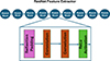 |
Fig. 6. Simplified visual representation of the ResNet Feature extractor. |
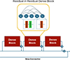 |
Fig. 7. Simplified visual representation of the improved DeepFilter Generator feature extractor, utilising RRDBs. The β functions represent the residual scaling parameter applied at each stage of learning. Each dense block in the figure is made up of dense layers as seen in Figure 8. |
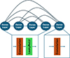 |
Fig. 8. Close-up of an individual dense block in the RRDB feature extractor as seen in Figure 7. Each layer can learn information from all previous layers, not just the previous one. |
As can be seen, the RRDB model has numerous changes in the architecture layout to make the feature extraction more precise. Unlike the nine consecutive residual blocks, the RRBD model uses three dense blocks each consisting of interconnected dense convolutional layers. Each of these blocks can then be added consecutively to the main training path. Additionally, these blocks can have their resulting residuals weighed by a residual scaling function when added to the training path (Lim et al. 2017). This function prevents instability in the model (Tai et al. 2017). A skip connector was also added to the architecture as this has been shown to allow the generator to detect and change more complex structures in the data (e.g. relatively fine coronal rain strands), as well as reduce any tendencies to mode collapse (Yang et al. 2020).
Another aspect in which the base CycleGAN algorithm proved inadequate for the AIA-IRIS style translation was in the algorithm’s tendency to add cross-hatch artefacts to the generated images. This is a well-known issue with CycleGANs: these errors occur in the up-sampling layers during forward propagation and in the down-sampling layers during back propagation (Kinoshita & Kiya 2020). These artefacts have a strong impact on the usability of the generated images for analysing coronal rain, as they distort the fine structures of the rain clumps, making them difficult to correctly identify. Work has already been done to solve this issue (Osakabe et al. 2021), and it was found that by inserting fixed convolutional layers to the up-sampling and down-sampling layers these artefacts can be avoided (Figure 9).
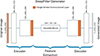 |
Fig. 9. Simplified visual representation of the improved DeepFilter Generator with added single-strided convolutional layers to avoid cross-hatch artefacts. |
3. Data
For training, the DeepFilter model uses training sets of 2000 images from AIA, and 2000 images taken from IRIS. The image sets consist of images of coronal rain taken from 20 different events between 19-11-2013 and 02-03-2024. The events were chosen to produce training images with diverse degradation levels from AIA over time, including coronal rain from a variety of sources (i.e. quiescent rain and flare-driven rain) and rain-free events. This ensures that the algorithm is not over-trained to expect rain always and thereby make rain where there is none. The events also contained coronal rain in a variety of locations on the Sun and at various orientations. Level 2 images of both AIA and of IRIS were used as image data for all images discussed in this paper. The calibrated IRIS data correspond to level 2 AIA data (including initial co-alignment and rotation for the two to match).
In the production of the training sets, we found significant imbalance between the number of coronal rain images taken with AIA than those taken with IRIS, with SDO observing continuously and IRIS having a more limited dataset length. Additionally, there is a significant imbalance between the number of images in specific events, possibly leading to over-training the algorithm to specific morphologies. To balance our dataset, an even split of the 2000 total images was taken from each event in both the AIA and IRIS observations. All AIA events contain well over this number of images, so creating an even split amongst the events is not a problem for this training set. However, for the IRIS observations some events only contain as few as twenty images, which is well below the split threshold. For these events, which do not have the required number of images to meet their allotted quota, image augmentation techniques are used to fill each event’s quota to the full training set. The image augmentations applied are random rotations and random shifting of images. These augmentations were chosen as they enable a variety of images to be produced without inherently changing the style and structure of the images that more extreme image augmentation processes carry out. Image augmentations such as these are a standard practice not only to increase the dataset size but also to promote generalisation over degrees of freedom known to be invariant (e.g. rotations) (Xu et al. 2023).
After this first stage of image augmentation, the images are loaded into the algorithm and undertake a second stage of image augmentation so as to maximise the generality of the training set. This is especially required for this domain as the training images come from specific events so large portions of the overall training set share significant similarities unrelated to the domain style, due to similar morphologies of images originating from the same event. Any process that minimises these non-style related similarities in the training data is incredibly useful to avoid over-fitting. During this second stage of image augmentation, the images go through a process of adding random jitter. Essentially, the images are reshaped to be slightly larger than the required size, then a random crop is taken in the desired image size. Additionally, the image is then randomly flipped both vertically and horizontally.
It was found that masking out the disk of the Sun was crucial to the algorithm’s success in enhancing rain observation off-limb. This was due to the fact that the off-limb material only accounts for a small fraction of the structure in the original images. As such, the algorithm tends to alter or sometimes completely remove this off-limb material to better process the on-limb structures and data. This is a known limitation for the purpose of this paper; therefore, the most efficient way of constraining the algorithm to focus on the off-limb material was to mask all the training data to remove any disk interference. For effective masking, a mask removing all values at solar radius less than 980 arcsec was used.
In the image augmentation pipeline, images are automatically renormalised to the [ − 1, 1] range, as in the original CycleGAN paper (Zhu et al. 2017), to centre the data and accelerate training of the neural networks. This is done automatically so that future images are not normalised prior to processing in the model.
4. Training and hyper-parameters
Utilising the model architecture – as described in Section 2.4 – then training the algorithm using the data detailed in Section 3 over the course of 200 epochs, a generalised model can be obtained to filter the hot component from unseen AIA 304 Å images. Over the training run, a series of hyper-parameters were tuned to increase the effectiveness of the DeepFilter algorithm. All optimal parameters were found by trialling a range of values for each parameter with the testing dataset to determine which combination gave the smallest total loss. Visual inspection of the resulting images was also carried out to find the optimal set of hyper-parameters.
4.1. Generator learning rate.
This is the rate at which the generator learns to make the style transfer from AIA to IRIS. It determines the magnitude of changes the algorithm can make to fit the style of the IRIS images. A value of 2 × 10⁻⁶ was found to be the optimal rate in this domain as the differences between styles is relatively small. The range of trialled values were between 1 × 10⁻⁷ and 1 × 10⁻⁴.
4.2. Discriminator learning rate.
Similarly to the generator learning rate, this parameter dictates the speed at which the discriminator learns to differentiate real and generated images. The optimal rate value is also 2 × 10⁻⁶. The range of trialled values were between 1 × 10⁻⁷ and 1 × 10⁻⁴.
4.3. Decay epoch.
The decay epoch is that in which the learning rate starts to reduce linearly to zero from the initial learning rates for both the generator and discriminator. This can help refine the model parameters in the later stages of training, improving the quality of the generated images. The optimal value was found to be the 100th epoch, with trials in the range of 20th to 150th epoch.
4.4. Size of feature map.
This dictates the number of defining features the algorithm picks out of the images to compare and change. For the Deep-filter algorithm a feature space of 64 × 64 was found to be optimal. The values of 32 and 128 were also trialled with less optimal results.
4.5. Patch size.
This is the size of patches the image is segmented into for the discriminator. A patch size of 70 × 70 was found to be optimal to take in the structural elements. The values of 35 and 140 were also trialled with less optimal results.
4.6. Cycle consistency.
Arguably the most changeable parameter in the algorithm dependent on the goal, this parameter dictates how close to the original image the algorithm wants to keep the generated image. It was found that a varying cycle consistency parameter performed best, due to the algorithm first needing to learn the overarching structures in the images (e.g. coronal loops prominences) before giving the algorithm more freedom to make smaller changes later in the training process to enhance the smaller structures in the image. As such, the algorithm was originally set to a cycle consistency parameter of 45 before decreasing to 40, then 30, and finally 20 at the 70th, 100th, and 150th epoch, respectively.
4.7. Identity consistency.
This is a secondary loss variable that dictates how much the algorithm prioritises the identity loss when training. This is the loss between the original image and the image produced when the target image is sent through a generator designed to convert to its own style. As per Liu (2022), a weight of 5 was found to be optimal.
5. Results
5.1. Evaluation observations
For evaluation it is crucial to choose a coronal rain event that had none of its constituent images used in the training of the algorithm. This is required to prevent a false sense of quality from the algorithm simply reproducing the steps in already seen images. We chose an event of coronal rain from 2014-03-13 of an AR off-limb captured by both AIA and IRIS as the test event due to its relatively early date in the lifespan of the instruments, so that degradation would be less pronounced. Additionally, the event included a C-class flare near the end of the observational sequence, which allowed us to further test for both the quiescent and flaring regimes. The co-observation ran from 01:34:39 UT to 03:23:00 UT. The FOV of the AIA images is 367″ × 382″ centred at (x, y) = (972″, 304″). The temporal resolution of the AIA images was 12 s with a plate scale of  per pixel. The IRIS observation programme for this dataset corresponds to the IHOP 248 programme (coordinated with Hinode), with OBSID 3840259254 consisting of a very large sit-and-stare (FOV of 166″ × 174″) using a small line list and included SJI 1400 Å and 2796 Å. The FOV was centred at the same point as its AIA counterpart, with a roll angle of 20°. Both available SJI channels were used, which have a cadence of 19 s, an exposure time of 8 s, and a plate scale of
  .
.
In addition to the IRIS images, the above AIA evaluation dataset was also processed using the temperature-based RFit algorithm (Antolin et al. 2024). This was done to compare the effectiveness of DeepFilter with current state-of-the-art models. Although RFit can provide both the cool and the hot components of an AIA passband, for simplicity we here refer to the cool AIA 304 Å component from RFit simply as the RFit AIA 304 Å component.
5.2. Evaluation pre- and post-processing
Before an image in the evaluation dataset is sent through DeepFilter, a few pre-processing steps are applied. These steps are in place with the aim of stabilising the Machine Learning algorithm and removing anomalies in the data that might confuse the model and generate vastly differing resulting images from the event dataset. The first step that is taken is any pixels above a threshold of 200 DN s−1 are saturated to this upper boundary. This step is crucial as the algorithm relies on a min-max normalisation. Pixels affected by cosmic rays having values several times higher than the uncontaminated pixels, when normalised these pixel values will cause the overall intensities of the DeepFiltered images to be altered relative to the rest of the images in the sequence, creating an inconsistent set of images. Secondly the background is removed from the image. The background for each image is found by taking an average of a portion of the image well away from the limb. This step reduces the effect of random noise within the images. Subsequently any negative value pixels are set to 0, as these will have an impact on the internal normalisation of the model if not removed. Thirdly the images are masked to only contain material above 980 arcsec to remove the disk as was done in the training images.
The final pre-processing step is the addition of a supplementary ‘stability’ bar to the image. This is an added small rectangle of width 35 pixels that is added to every image on the side of the image furthest from the limb. This bar is populated with segments of various intensities ranging from a few DN per second to the image maximum of 200 DN s−1. Crucially, this stability bar provides intensity consistency for all images in the evaluation dataset. An example of this stability bar can be seen in Figure 10. The addition of this stability bar forces the algorithm to not make wildly different decisions between one image in the sequence and the next, keeping the resulting relative intensities consistent. Without this stability bar in place what might be considered the threshold for a bright pixel in one image can be vastly different in the following image. This effect is particularly egregious when any form of intense brightening is observed in the event, which generally occurs during flaring events.
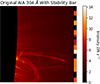 |
Fig. 10. Example image including the stability bar, taken from the evaluation dataset after the pre-processing steps were applied prior to being DeepFiltered. |
Once an image has been filtered for hot material by DeepFilter, it is output as a 2D array normalised between −1 and 1, with the stability bar still present in the image. As the stability bar is an additional bar, it can simply be removed post-filtering. To convert the images back to the original units, the minimum and maximum of the original image prior to the stability bar’s addition were found and used to renormalise the image, as these were the values used in the original normalisation. Additionally, any pixels assigned negative values were saturated to 0.
To successfully carry out any evaluation of the model either qualitatively or quantitatively, the AIA images must be precisely co-aligned with their IRIS counterparts as well as with each other. It was found that if some of the EUV images are misaligned even by a few pixels the RFit algorithm’s ability to remove the correct material can be severely affected. This is carried out by utilising the heliocentric coordinate system provided in each FITS file and making sub-maps of AIA of the matching coordinates supplied to each FITS file by LMSAL. This allows a rough AIA cutout to be made, which corresponds to the size of the area of the Sun captured by the IRIS images, as well as the approximate location. Small misalignments of a few pixels usually persist. This slight misalignment was manually removed to produce sub-pixel co-alignment accuracy between the images. In addition to making sure that spatially all AIA 304 Å images match IRIS 1400 Å, all images need to be temporally matched. As coronal rain is a highly dynamic phenomenon, the images need to be as closely temporally coordinated as possible. For each timestamp in the IRIS 1400 Å image, the closest image in the AIA EUV channel is selected, based on its timestamps. Once the adjustment for the slight misalignment and removal of unmatched images is carried out, the corresponding cutout of the IRIS image can be taken from any AIA image, as seen in Figure 1.
IRIS images are higher resolution than those taken by AIA by a factor of ≈1.8 or ≈3.6, depending on the dataset. As a result, structures appear much finer in IRIS when the two are compared (Şahin et al. 2023). For the purpose of comparing the material captured by each instrument, it is imperative to reduce the spatial resolution of the IRIS images to match that of AIA. This is performed by applying Gaussian smoothing with a full width half maximum (FWHM) of 1.8 to mimic the effect of the coarse point spread function from AIA. An additional median filter of kernel size 4 was added to all image types to reduce the effects of background noise. For the IRIS images this median filter was applied before the Gaussian smoothing was applied.
5.3. Identifying cool material in images
The primary goal of DeepFilter is to enable easier identification of cool coronal material. With that goal in mind an intensity threshold must be found that can optimally separate cool material from the background noise. To do this, we used the IRIS 2796 Å images (which are not affected by hot emission) as ground truth for the presence of cool emission. The 2796 Å images were manually binarised to determine a threshold, which encompasses the maximum amount of rain while removing noise. For the remaining image types (from IRIS 1400 Å the original AIA 304 Å and the corresponding RFit and DeepFilter versions), the optimal intensity threshold, which encompasses the maximum amount of cool material while removing any noise or low-intensity emission, was found by calculating the Pearson correlation coefficient between each binarised image at multiple threshold values and the corresponding IRIS 2796 Å binarised image in the dataset. This was carried out at a range of intensity thresholds between 0−30 DN s−1 and the threshold corresponding to the maximum correlation coefficient chosen as the optimal threshold value going forward. The results of this process are shown in Figure 11, which shows how the correlation changes depending on the specific threshold chosen. It is worth noting that some coronal rain appearing in IRIS 1400 Å may not appear in IRIS 2796 Å, since the latter forms at cooler temperatures of [1 − 2]×104 K or less. However, observations and numerical simulations indicate that most of the rain usually cools down all the way to that temperature regime (Şahin et al. 2023; Antolin et al. 2022), and therefore we expect that the correlation is not too much affected.
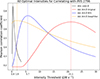 |
Fig. 11. Figure showing how the optimal threshold for each image type was found. Each image type (IRIS 1400, Original AIA 304 Å RFit AIA 304 Å Deep Filter AIA 304 Å) is binarised at a range of intensity thresholds between 0.1 and 30 DN s−1. For each 0.1 DN s−1 step in this range, the binarised images are correlated with the pre-binarised IRIS 2796 images for the entirety of the evaluation dataset. The resulting correlation coefficients are calculated and then plotted. The threshold for each image type can then be found and are indicated by the dotted lines in the figure. |
The optimal intensity thresholds were calculated for all image types and were found to be 0.4 DN s−1, 21.1 DN s−1, 5.7 DN s−1, 1.9 DN s−1, and 0.17 DN s−1, respectively, for the IRIS 1400 Å, the original AIA 304 Å, the RFit AIA 304 Å, the DeepFilter AIA 304 Å, and the IRIS 2796 Å images. In order to remove any pixel values corresponding to cosmic rays an upper threshold was also applied to the images of 200 DN s−1 and 1000 DN s−1 for the AIA and IRIS images, respectively.
5.4. Qualitative results
For the evaluation of the success of DeepFilter in removing the hot component from AIA 304 Å images, a qualitative comparison can be made between the images produced by RFit and DeepFilter on the evaluation dataset, along with those of the original AIA 304 Å images and IRIS 1400 Å and 2796 Å. To better identify the similarities and differences across the images, we highlighted the pixels present only in either IRIS 1400 Å or AIA 304 Å (original, RFit and DeepFilter), and those present in both. This is shown in Figures 12, 13, 14 and 15, respectively, at times of quiescent rain, the flare impulsive time, the beginning of the flare-driven rain, and during the flare-driven rain. Besides the difference images between AIA and IRIS 1400 Å, these figures include the images and the corresponding binarised versions.
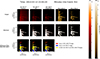 |
Fig. 12. Snapshot of how the various algorithms perform in the evaluation dataset. Top, from left to right: Original, RFit, and DeepFilter AIA 304 Å as well as the IRIS 1400 Å and 2796 Å images produced at a time with quiescent coronal rain. The AIA images use 0.5 power scaling, while the IRIS images use 0.3 power scaling. Middle: Same images binarised by the optimal threshold found in Section 5.3. Bottom: Differences and similarities between the AIA 304 Å and IRIS 1400 Å binarised images (see legend for colour scheme used). |
Generally, DeepFilter and RFit produce similar results and are successful at removing the hot emission, particularly when compared to the unprocessed AIA 304 Å images. This is exemplified by Figure 12, with the most obvious difference being the processed AIA images containing far more substructures particularly closer to the limb when compared to the original images thanks to the large gain in contrast. This translates into an increase in pixels in the binarised images. From a visual standpoint, DeepFilter produces higher contrast images compared to RFit.
The largest difference between the two algorithms can be observed specifically in Figure 13 at the time of the flare, and in Figure 14 at the beginning of the flare-driven rain. In Figure 13 we can see that DeepFilter removes or narrows the fine rain strands, particularly further away from the limb. Additionally, the apex of the flare loop at (x, y)≈(1000″, 300″) that appears in the IRIS 1400 Å due to the hot Fe XXI emission is not properly removed by RFit but is successfully removed by DeepFilter. In Figure 14 the flare-driven coronal rain starts to appear in the loop and is fully captured by DeepFilter but far less by RFit. Considering that this structure is absent in both of the IRIS channels suggests that the material has cooled down to temperatures of around 105 K but not lower. As DeepFilter relies entirely on the morphological separation of the hot from the cool component, the algorithm does not remove this 105 K component since it is morphologically similar to the colder coronal rain forming a few minutes later. Accordingly, the DeepFilter and RFit images in Figure 15 during the flare-driven rain appear almost exactly the same.
5.5. Quantitative results
The qualitative results seen in Section 5.4 show that DeepFilter appears to be generally successful in its primary goal of hot-component removal. We now conduct a more quantitative analysis of the algorithm’s performance. This analysis needs to support the two important characteristics identified in the prior qualitative analysis. First, it needs to show that the algorithm effectively removes the hot diffuse material in the AIA 304 Å and, second, that the resulting image preserved the underlying structure of the coronal rain. An evaluation technique that covers both points utilises a correlation analysis of the structures seen in the AIA images before and after hot-component removal, compared to the coronal structures seen in IRIS.
For this assessment, the binarised images produced – as discussed in Section 5.3 – are directly compared, with all binarised image sets Pearson-correlated against both IRIS 1400 Å and 2796 Å. The correlation was carried out for all images in the event and is plotted in Figure 16. This enables temporal analysis of how the algorithms perform over the image set.
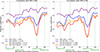 |
Fig. 16. Correlation plots showing the Pearson correlation coefficients between the various binarised AIA-based images and the IRIS-based images (left: IRIS 1400 Å; right: IRIS 2796 Å). The average Pearson correlation coefficient is shown in the bottom left of each graph. |
The plots shown in Figure 16 back up the qualitative results shown in Section 5.4 in so much as both hot-component removal algorithms show an improvement in the correlation with both IRIS channels compared to the original AIA 304 Å images, implying that both are effective at reducing the impact of the hot component. Overall, RFit produces a greater correlation, particularly in the timestamps of the event encapsulated by Snapshot Two shown in Figure 13 and Snapshot Three shown in Figure 14.
In Figure 17 the total number of pixels associated with cool plasma at coronal heights is calculated based on the aforesaid thresholds. In the trends seen in the figure, RFit appears to follow the trends of the IRIS data more closely than DeepFilter, with the latter appearing to follow more closely the distribution found in the original images. Looking at the normalised counts on the right panel of the figure, there is a more obvious difference in the pixels being counted by each image type. The RFit images seem to match the overall trend in the cool material over the event seen in IRIS to a greater extent than DeepFilter, with clear minima at approximately 20 min and 80 min into the event, and local maxima seen at approximately 50 min into the event similar to the trend seen in the IRIS image sets.
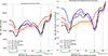 |
Fig. 17. Counts of rain-like pixels in each image of the evaluation event, where each has an intensity value within the expected threshold (see text for details). Left: Un-normalised distribution. Right: Normalised distribution over time. |
These Figures give a partial view on how the hot-component removal algorithms perform. Another key information is whether the algorithm is over- or under-removing material, as both false-positives and false-negatives have the same effect on the overall score. To more thoroughly see the effects of each algorithm on the material in the AIA images, we show in Figure 18 a count over the event for pixels only belonging to the AIA or to the IRIS images. The left panel of the figure corresponds to the red pixels seen in the difference images of Figures 12–15, namely appearing only in IRIS 1400 Å, whilst the right panel corresponds to the blue pixels in these snapshots, namely appearing only in AIA 304 Å.
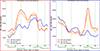 |
Fig. 18. Counts of rain-like pixels in each image of the evaluation event that either exclusively belong to the IRIS 1400 Å image and are absent in the AIA images (i.e. false negatives, left), or exclusively belong to the AIA 304 Å image type and are absent in IRIS 1400 Å (i.e. false positives, right). |
A few aspects of these plots show how the different algorithms perform. First, we can see that both algorithms’ performances vary over the course of the event. For the first approximately 80 minutes of the event, both algorithms outperform the original images in false negatives observed, with both having less than the original images. The RFit algorithm performs particularly well in this regard over the time frame. This is likely due to the amount of fine substructures that the RFit algorithm does a great job at preserving, which have been reduced in the binarised DeepFiltered images and completely removed in the binarised original images (see Figure 13). In the same panel, after 80 minutes of the event, both algorithms show an overall increase in false negatives relative to unprocessed images, with the DeepFiltering algorithm appearing to outperform RFit by not over-removing during this period. This period of the event is no longer dominated by smaller structures. Rather, the rain is mostly confined to larger loops. It is in these loops that the over-removal of both the algorithms is seen with both reducing the observed width of the loops, particularly closer to the limb (see Figure 15). Moving on to the right panel of the figure, which depicts the false positives for the first 60 minutes of the event, both algorithms appear to show more false positives than the original images. However, the difference here is not large and is more likely a result of the slight mismatch in observed structure between AIA 304 Å and IRIS 1400 Å. The more dramatic difference between the algorithms can be seen after this 60 minute mark where the number of false positive pixels increases dramatically in both the original images and the DeepFiltered images, though the original images see a greater rise than the DeepFilter images. This is stark against the RFit images, which have a mostly declining false positive rate in this period. This divergence in the algorithms is a result of the morphological change in the evaluation dataset, specifically between 60 − 90 min into the event where the DeepFilter AIA 304 Å images show a complete coronal loop either absent from or incomplete in the IRIS or RFit images.
The final aspect to analyse in the methodology is how DeepFilter changes the intensity values in the overall coronal structures. To investigate this, we calculated the mean pixel intensities corresponding to only the pixels shared by all image types and show the time evolution in Figure 19. The trends in these mean pixel intensities can then be compared against one another. In this figure, it can be seen that RFit and DeepFilter produce similar results with clear reductions in the mean pixel intensities when compared to the unprocessed AIA 304 Å images. This implies that both remove material present in the original images. Both the original and RFit AIA 304 Å images show the same trend in mean pixel intensities and are only shifted by a roughly equal amount over time. The same cannot be said for the trend in intensities for DeepFilter. In fact the mean intensity trend observed in this method appears to be an amalgamation in the trends observed in AIA 304 Å and those observed in IRIS. This highlights that the DeepFilter algorithm goes beyond its remit of removing the hot component and modifies the relative intensities of the cooler structure to match those seen in IRIS.
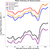 |
Fig. 19. Temporal evolution of the mean intensity for rain-like pixels shared by all image types. |
6. Discussion
From both a quantitative and qualitative stand-point, both the RFit and the DeepFilter algorithms produce improved results compared to the unprocessed AIA 304 Å images. Both methodologies efficiently remove the hot component seen in the AIA 304 Å channel, obtaining correlations with IRIS higher than those achieved by the original AIA 304 Å images. Despite the apparent similarity in the qualitative results of both methods, there are a number of significant differences between the images produced that act as advantages or disadvantages for each algorithm.
6.1. RFit
The RFit method produces very high average correlation scores with IRIS for both channels tested over the evaluation event, with average correlations of 0.755 and 0.747 with IRIS 1400 Å and 2796 Å, respectively. This approach has broadly three major disadvantages – all related to the fact that it depends on the availability of the other EUV channels (and at least three, namely, AIA 94 Å, 211 Å, and 335 Å; Antolin et al. 2024). First, it requires correctly weighing the various other EUV channels to approximate the hot-component temperature response of AIA 304 Å. This approximation is never entirely accurate and does lead to the under- or over-removal of material. Additionally, the temperature responses of the various EUV channels are not static and will change significantly over the course of AIA’s observational lifetime due to degradation. This means that the weights will vary with similar timescales as that of degradation (of a year or less). Finally, besides the original AIA 304 Å image, the other EUV images are also needed (particularly AIA 94 Å, 211 Å, and 335 Å). Adding to the overall data size needed to produce the RFit image, the efficiency of RFit will suffer from potential misalignments between the AIA EUV images. Conversely, this approach has a number of significant advantages. Apart from exhibiting the largest improvement in the correlations with IRIS, it is also morphologically blind in its approach by only basing its result in the temperature response functions. This enables its use in full-disk AIA 304 Å images without being mislead by morphologies indistinct in the original AIA 304 Å images from other cool structures, such as the compact hot emission from flare loops observed in Figure 14.
6.2. DeepFilter
The DeepFilter method also produces high average correlation scores with both IRIS channels of 0.717 and 0.692 for IRIS 1400 Å and 2796 Å, respectively. Although lower on average than the RFit method, this is still a marked improvement in the cool material identification compared to the unprocessed AIA 304 Å images. This algorithm has a few significant disadvantages, the first of which is that it relies entirely on the morphology of the structures in the image to identify whether or not it is cool material (which is the reason for the lower correlation with the IRIS images). In this sense, it can be easily fooled by hot compact emission such as that seen in Figure 14, leading to an under-removal of this material. Another failing of the model is that it is poor at identifying faint cool material particularly far away from the limb. This can be seen in Figure 13, whereby faint material away from the limb is either narrowed or removed entirely, leading to an over-removal of this material. The way that this model has been trained also limits the versatility of the technique, as it can only be used on limb snapshots and not on full-disk images. This is due to the training set relying on IRIS images, which only provide a small FOV, making DeepFilter only applicable to equivalent snapshots. This disadvantage can be circumvented somewhat by first splitting a full-disk image into a mosaic of snapshots, then processing with a DeepFilter, and finally reassembling; however, this requires more time and is a computationally consuming workaround. The primary advantage of this methodology over RFit is that, once trained, DeepFilter does not require any additional data other than the original AIA 304 Å image for processing. This significantly reduces the data size and pre-processing required to produce cool AIA 304 Å images.
As the DeepFilter method relies heavily on the training data used, many of the disadvantages discussed prior can be mitigated by improvements in the training model. Due to the relatively low-powered GPU used for training the machine (Nvidia RTX 3080, 32GB RAM), the input training data were constrained to 2000 images of each image type (AIA 304 Å and IRIS 1400 Å), while only being able to run 200 epochs. Although this has shown to be mostly sufficient in producing images that show a clear reduction in hot-component material, this has limited the sensitivity of the model particularly when faint cool material is present. The computational constraints have also forced the training images to be of size 512 × 512 pixels. Although this does not translate into a huge change in resolution for the AIA 304 Å training images used, it does mean that some of the finer structures may be missed. It is worth reiterating that although the training images must be this size, the model can be used on any size of AIA image once the style translation has been learned. A full comparative ablation study is reserved for a future publication to pinpoint which component (e.g. disk occlusion, architecture changes, and stability bar) was the main driver of improvement to the underlying model. Finally, as discussed in Section 3, a relatively limited diversity of IRIS coronal rain images, with available data constrained to a few large high-cadence events, currently exists. Only 20 separate events were used to make the 2000-image training set; ideally this number would be closer to 100. In practice, this limits how general DeepFilter can be as it can easily be over-fit to particular morphologies seen in the current IRIS image datasets. Although data augmentation procedures have been carried out in this paper they can only go so far in avoiding over-fitting on this data.
6.3. The use of IRIS
For both quantitative and qualitative results and interpretation, IRIS 1400 Å and 2796 Å have been assumed to reliably represent the ground truth for the real, cool material that should be present. However, this assumption has some important caveats. The first point that both IRIS channels share is that both channels do not entirely capture the same temperature range as AIA 304 Å. IRIS 1400 Å and 2796 Å form at ≈104.8 K and ≈104 K, respectively, and are much sharper peaked in temperature than AIA 304 Å, which forms at 105 K. Therefore, some discrepancy in the material observed is to be expected. It is also important to note that the IRIS 1400 Å channel has a hot component from Fe XXI emission at ≈107 as seen in Figure 2. The effect of this hot component can be seen in Figure 13 of the evaluation dataset, which captures the flaring stage. The flare loop appears as a diffuse structure near the top of the IRIS 1400 Å image and corresponding binarised image, and is absent from the IRIS 2796 Å. The presence of this hot emission in the DeepFilter image means that RFit does a better job than DeepFilter at removing hot-component material at this time-step. However, the impact of this IRIS 1400 Å hot component is not significant. Another important difference between the channels is the large difference in opacity in the dominant spectral lines. The He II 304 Å spectral line is significantly more opaque and is often optically thick (Golding et al. 2017) than the optically thin Si IV 1393 Å and 1402 Å lines. This makes the coronal rain appear more prominent in AIA 304 Å than in IRIS 1400 Å, which naturally leads to a reduction in the correlation.
7. Conclusion
In this paper a novel approach was proposed to remove the diffuse material associated with the hot component of the AIA 304 Å channel, whose main contribution peaks at T ≈ 106.2 K. The aim of this method is to produce images with emission solely belonging to the channel’s cool component (T ≈ 105 K). The approach proposed within this paper makes use of the fact that another instrument, namely IRIS, provides a more disambiguated picture of the temperature of the plasma and better captures the cool coronal emission from material such as coronal rain. Accordingly, IRIS 1400 Å produces images with far greater contrast between the cool plasma, constituting the rain, and the background. A machine-learning algorithm based on a CycleGAN was developed that learns how to translate between the cool and hot components based on their morphological difference, with the express aim of improving rain contrast in the AIA 304 Å images and thereby eliminating hot-component impact. The resulting images were then compared to the recent RFit method (Antolin et al. 2024), which is temperature-based and utilises the temperature response functions of the other EUV channels to recreate and remove the hot AIA 304 Å component.
In general, the proposed methodology is successful at removing the hot-component emission from the AIA 304 Å images, enabling better identification and quantification of off-limb cool material, such as coronal rain, prominences, and spicules. When compared to RFit, we show that it produces comparable but slightly inferior results, particularly by over-removing faint cool emission, and being unable to differentiate the hot compact emission from, for example, flare loops. Despite this, it has still been shown to produce comparable results without requiring any additional data or calculations as for RFit. Many of the shortcomings in the model can likely be addressed by utilising a larger, more diverse training dataset that better tests degradation impacts and model adjustments to account for these image types. However, due to computational limitations, this could not be tested in this study. Future applications of this model are diverse and include large-scale statistical analyses into the causes and effects of the cool material in the corona. This will be the subject of future work.
Acknowledgments
The data used is courtesy of SDO and IRIS. SDO is a mission for NASA’s Living With a Star (LWS) program. IRIS is a NASA small explorer mission developed and operated by LMSAL with mission operations executed at NASA Ames Research Center and major contributions to downlink communications funded by ESA and the Norwegian Space Centre. This research was supported by the International Space Science Institute (ISSI) in Bern, through ISSI International Team project #545 (‘Observe Local Think Global: What Solar Observations can Teach us about Multiphase Plasmas across Physical Scales’). This research used version 7.0.3 (Mumford et al. 2025) of the SunPy open source software package (The SunPy Community 2020). LM acknowledges the UK Research and Innovation (UKRI) Science and Technology Facilities Council (STFC) for support from grant No. ST/W006790/1 and for IDL support. This study has been supported by the STFC Centre for Doctoral Training in Data Intensive Science (NUdata), as a collaboration between Northumbria and Newcastle Universities. All data used in this paper is available upon reasonable request. The research was sponsored by the DynaSun project and has thus received funding under the Horizon Europe programme of the European Union under grant agreement (no. 101131534). Views and opinions expressed are however those of the author(s) only and do not necessarily reflect those of the European Union and therefore the European Union cannot be held responsible for them. This work was also supported by the Engineering and Physical Sciences Research Council (EP/Y037464/1) under the Horizon Europe Guarantee. We also kindly thank the referee of this paper for providing excellent feedback.
References
- Antiochos, S., DeVore, C., & Klimchuk, J. 1999, ApJ, 510, 485 [Google Scholar]
- Antolin, P. 2019, Plasma Phys. Controlled Fusion, 62, 014016 [Google Scholar]
- Antolin, P., & Froment, C. 2022, Front. Astron. Space Sci., 9, 820116 [NASA ADS] [CrossRef] [Google Scholar]
- Antolin, P., Shibata, K., & Vissers, G. 2010, ApJ, 716, 154 [NASA ADS] [CrossRef] [Google Scholar]
- Antolin, P., Vissers, G., & Rouppe van der Voort, L. 2012, Sol. Phys., 280, 457 [NASA ADS] [CrossRef] [Google Scholar]
- Antolin, P., Vissers, G., Pereira, T., van der Voort, L. R., & Scullion, E. 2015, ApJ, 806, 81 [NASA ADS] [CrossRef] [Google Scholar]
- Antolin, P., Martínez-Sykora, J., & Şahin, S. 2022, ApJ, 926, L29 [NASA ADS] [CrossRef] [Google Scholar]
- Antolin, P., Auchère, F., Winch, E., Soubrié, E., & Oliver, R. 2024, Sol. Phys., 299, 94 [NASA ADS] [CrossRef] [Google Scholar]
- Asperti, A., & Tonelli, V. 2023, Neural Comput. Appl., 35, 3155 [Google Scholar]
- Claes, N., & Keppens, R. 2019, A&A, 624, A96 [NASA ADS] [CrossRef] [EDP Sciences] [Google Scholar]
- De Pontieu, B., Title, A., Lemen, J., et al. 2014, Sol. Phys., 289, 2733 [NASA ADS] [CrossRef] [Google Scholar]
- Del Zanna, G., Dere, K., Young, P., & Landi, E. 2021, ApJ, 909, 38 [NASA ADS] [CrossRef] [Google Scholar]
- Dufresne, R., Del Zanna, G., Young, P., et al. 2024, ApJ, 974, 71 [Google Scholar]
- Fan, C., Lin, H., & Qiu, Y. 2023, J. Digit. Imaging, 36, 339 [Google Scholar]
- Fontenla, J., Landi, E., Snow, M., & Woods, T. 2014, Sol. Phys., 289, 515 [Google Scholar]
- Froment, C., Auchère, F., Aulanier, G., et al. 2017, ApJ, 835, 272 [Google Scholar]
- Golding, T. P., Leenaarts, J., & Carlsson, M. 2017, A&A, 597, A102 [NASA ADS] [CrossRef] [EDP Sciences] [Google Scholar]
- Goodfellow, I., Pouget-Abadie, J., Mirza, M., et al. 2014, Adv. Neural Inf. Process. Syst., 27 [Google Scholar]
- Isola, P., Zhu, J. Y., Zhou, T., & Efros, A. A. 2017, Proceedings of the IEEE Computer Society Conference on Computer Vision and Pattern Recognition, 1125 [Google Scholar]
- Karpen, J., Antiochos, S., Hohensee, M., Klimchuk, J., & MacNeice, P. 2001, ApJ, 553, L85 [Google Scholar]
- Keppens, R., De Jonghe, J., Kelly, A., Brughmans, N., & Goedbloed, H. 2025, ApJ, 989, 51 [Google Scholar]
- Kinoshita, Y., & Kiya, H. 2020, Proc. – ICASSP IEEE International Conference on Acoustics, Speech, and Signal Processing (IEEE), 3712 [Google Scholar]
- Kleint, L., Antolin, P., Tian, H., et al. 2014, ApJ, 789, L42 [NASA ADS] [CrossRef] [Google Scholar]
- Klimchuk, J. A. 2006, Sol. Phys., 234, 41 [Google Scholar]
- Klimchuk, J. A., & Luna, M. 2019, ApJ, 884, 68 [Google Scholar]
- Kohutova, P., Antolin, P., Popovas, A., Szydlarski, M., & Hansteen, V. 2020, A&A, 639, A20 [NASA ADS] [CrossRef] [EDP Sciences] [Google Scholar]
- Lemen, J. R., Title, A. M., Akin, D. J., et al. 2012, Sol. Phys., 275, 17 [Google Scholar]
- Lim, B., Son, S., Kim, H., Nah, S., & Mu Lee, K. 2017, Proceedings of the IEEE Conference on Computer Vision and Pattern Recognition (CVPR), 136 [Google Scholar]
- Lionello, R., Winebarger, A. R., Mok, Y., Linker, J. A., & Mikić, Z. 2013, ApJ, 773, 134 [NASA ADS] [CrossRef] [Google Scholar]
- Liu, S. 2022, J. Phys. Conf. Ser., 2400, 012030 [Google Scholar]
- Liu, Y., Jun, E., Li, Q., & Heer, J. 2019, Comput. Graph. Forum., 38, 67 [Google Scholar]
- Mumford, S. J., Freij, N., Stansby, D., et al. 2025, https://doi.org/10.5281/zenodo.591887 [Google Scholar]
- O’Dwyer, B., Del Zanna, G., Mason, H., Weber, M., & Tripathi, D. 2010, A&A, 521, A21 [Google Scholar]
- Osakabe, T., Tanaka, M., Kinoshita, Y., & Kiya, H. 2021, International Workshop on Advanced Imaging Technology (IWAIT) 2021, 11766, 51 [Google Scholar]
- Şahin, S., Antolin, P., Froment, C., & Schad, T. A. 2023, ApJ, 950, 171 [CrossRef] [Google Scholar]
- Tai, Y., Yang, J., & Liu, X. 2017, IEEE Conference on Computer Vision and Pattern Recognition (CVPR), 3147 [Google Scholar]
- Taigman, Y., Polyak, A., & Wolf, L. 2017, 5th International Conference on Learning Representations, ICLR 2017 – Conference Track Proceedings [Google Scholar]
- The SunPy Community (Barnes, W. T., et al.) 2020, ApJ, 890, 68 [Google Scholar]
- Thompson, W. T., & Brekke, P. 2000, Sol. Phys., 195, 45 [NASA ADS] [CrossRef] [Google Scholar]
- Tousey, R., Austin, W. E., Purcell, J. D., & Widing, K. G. 1965, Ann. Astrophys., 28, 755 [NASA ADS] [Google Scholar]
- Wang, T., & Lin, Y. 2024, ArXiv e-prints [arXiv:2408.15374] [Google Scholar]
- Wang, X., Yu, K., Wu, S., et al. 2018, Proceedings of the IEEE International Conference on Computer Vision [Google Scholar]
- Waters, T., & Stricklan, A. 2025, Sol. Phys., 300, 5 [Google Scholar]
- Xia, C., Chen, P., Keppens, R., & van Marle, A. J. 2011, ApJ, 737, 27 [NASA ADS] [CrossRef] [Google Scholar]
- Xia, C., Keppens, R., Antolin, P., & Porth, O. 2014, ApJ, 792, L38 [Google Scholar]
- Xu, M., Yoon, S., Fuentes, A., & Park, D. S. 2023, Pattern Recognit., 137, 109347 [NASA ADS] [CrossRef] [Google Scholar]
- Yang, Y., Jin, R., & Xu, C. 2020, Proceedings of the 2020 4th International Conference on Computer Science and Artificial Intelligence, 57 [Google Scholar]
- Yoshihisa, T., Yokoyama, T., & Kaneko, T. 2024, ApJ, 978, 94 [Google Scholar]
- Zhao, J., Mathieu, M., & LeCun, Y. 2017, 5th International Conference on Learning Representations, ICLR 2017 – Conference Track Proceedings [Google Scholar]
- Zhu, J. Y., Park, T., Isola, P., & Efros, A. A. 2017, Proceedings of the IEEE International Conference on Computer Vision, 2223 [Google Scholar]
All Figures
|
Fig. 1. Examples of AIA (left) and IRIS (right) co-aligned images of the same coronal rain event. As can be seen, the AIA contains a much greater amount of diffuse material due to the contribution of the hot component of its temperature response. In contrast, the coronal rain structures in the IRIS image are much more easily differentiated from the surroundings. |
| In the text | |
|
Fig. 2. Temperature response functions for the AIA 304 Å and IRIS 1400 Å channels. It is worth noting that the response function was calculated based on the CHIANTI database, which has been known to fail at reproducing the He II intensity peak between 104.8–104.9 K, where the resulting peak is an order of magnitude lower. This is likely due to the effects of non-equilibrium ionisation in tandem with optically thick radiative transfer in the He II line causing these large intensities (Golding et al. 2017). To account for this, the AIA 304 Å response function has been multiplied by an empirical factor of 5 (O’Dwyer et al. 2010). |
| In the text | |
|
Fig. 3. Simplified diagram of a typical training iteration of the DeepFilter algorithm. The diagram is colour-coded to show where each loss function is calculated. Red denotes adversarial loss, purple denotes cycle consistency loss, and green denotes identity loss. The equation where these losses are then used to calculate the total loss during the training is Eq. (5). |
| In the text | |
|
Fig. 4. Simplified visual representation of the basic architecture of the CycleGAN Generator. |
| In the text | |
|
Fig. 5. Simplified visual representation of the basic architecture of the base CycleGAN Discriminator. |
| In the text | |
|
Fig. 6. Simplified visual representation of the ResNet Feature extractor. |
| In the text | |
|
Fig. 7. Simplified visual representation of the improved DeepFilter Generator feature extractor, utilising RRDBs. The β functions represent the residual scaling parameter applied at each stage of learning. Each dense block in the figure is made up of dense layers as seen in Figure 8. |
| In the text | |
|
Fig. 8. Close-up of an individual dense block in the RRDB feature extractor as seen in Figure 7. Each layer can learn information from all previous layers, not just the previous one. |
| In the text | |
|
Fig. 9. Simplified visual representation of the improved DeepFilter Generator with added single-strided convolutional layers to avoid cross-hatch artefacts. |
| In the text | |
|
Fig. 10. Example image including the stability bar, taken from the evaluation dataset after the pre-processing steps were applied prior to being DeepFiltered. |
| In the text | |
|
Fig. 11. Figure showing how the optimal threshold for each image type was found. Each image type (IRIS 1400, Original AIA 304 Å RFit AIA 304 Å Deep Filter AIA 304 Å) is binarised at a range of intensity thresholds between 0.1 and 30 DN s−1. For each 0.1 DN s−1 step in this range, the binarised images are correlated with the pre-binarised IRIS 2796 images for the entirety of the evaluation dataset. The resulting correlation coefficients are calculated and then plotted. The threshold for each image type can then be found and are indicated by the dotted lines in the figure. |
| In the text | |
|
Fig. 12. Snapshot of how the various algorithms perform in the evaluation dataset. Top, from left to right: Original, RFit, and DeepFilter AIA 304 Å as well as the IRIS 1400 Å and 2796 Å images produced at a time with quiescent coronal rain. The AIA images use 0.5 power scaling, while the IRIS images use 0.3 power scaling. Middle: Same images binarised by the optimal threshold found in Section 5.3. Bottom: Differences and similarities between the AIA 304 Å and IRIS 1400 Å binarised images (see legend for colour scheme used). |
| In the text | |
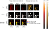 |
Fig. 13. Same as in Figure 12 at the time of the flare. |
| In the text | |
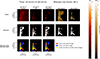 |
Fig. 14. Same as in Figure 12 at the beginning of the flare-driven rain. |
| In the text | |
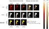 |
Fig. 15. Same as in Figure 12 during the flare-driven rain. |
| In the text | |
|
Fig. 16. Correlation plots showing the Pearson correlation coefficients between the various binarised AIA-based images and the IRIS-based images (left: IRIS 1400 Å; right: IRIS 2796 Å). The average Pearson correlation coefficient is shown in the bottom left of each graph. |
| In the text | |
|
Fig. 17. Counts of rain-like pixels in each image of the evaluation event, where each has an intensity value within the expected threshold (see text for details). Left: Un-normalised distribution. Right: Normalised distribution over time. |
| In the text | |
|
Fig. 18. Counts of rain-like pixels in each image of the evaluation event that either exclusively belong to the IRIS 1400 Å image and are absent in the AIA images (i.e. false negatives, left), or exclusively belong to the AIA 304 Å image type and are absent in IRIS 1400 Å (i.e. false positives, right). |
| In the text | |
|
Fig. 19. Temporal evolution of the mean intensity for rain-like pixels shared by all image types. |
| In the text | |
Current usage metrics show cumulative count of Article Views (full-text article views including HTML views, PDF and ePub downloads, according to the available data) and Abstracts Views on Vision4Press platform.
Data correspond to usage on the plateform after 2015. The current usage metrics is available 48-96 hours after online publication and is updated daily on week days.
Initial download of the metrics may take a while.