| Issue |
A&A
Volume 707, March 2026
|
|
|---|---|---|
| Article Number | A1 | |
| Number of page(s) | 17 | |
| Section | Stellar structure and evolution | |
| DOI | https://doi.org/10.1051/0004-6361/202558057 | |
| Published online | 25 February 2026 | |
Local simulations of common-envelope dynamical inspiral
Impact of rotation, accretion, and stratification
1
Zentrum für Astronomie der Universität Heidelberg, Astronomisches Rechen-Institut Mönchhofstr. 12-14 D-69120 Heidelberg, Germany
2
Heidelberger Institut für Theoretische Studien Schloss-Wolfsbrunnenweg 35 69118 Heidelberg, Germany
3
Zentrum für Astronomie der Universität Heidelberg, Institut für Theoretische Astrophysik Philosophenweg 12 69120 Heidelberg, Germany
★ Corresponding author: This email address is being protected from spambots. You need JavaScript enabled to view it.
Received:
11
November
2025
Accepted:
4
January
2026
Abstract
Common envelope evolution is a crucial phase in binary stellar evolution. Current global three-dimensional simulations lack the resolution to capture the small-scale dynamics around the embedded companion, while local wind-tunnel simulations always approximate the companion’s orbital motion as linear rather than as rotation around the center of mass. We investigated how rotation, accretion, and stratification influence small-scale gas dynamics, gravitational drag and lift forces, and the spin-up rate of the companion. We performed three-dimensional local hydrodynamic simulations of a 0.2 M⊙ compact companion plunging into the envelope of a 2 M⊙ red giant in a reference frame rotating at the companion’s orbital angular velocity, using the Athena++ code. The presence of stratification generates an inward directed force, which is partially opposed by a rotation-induced outward lift force. Both the resulting inward directed force and the drag force, strongly influenced by stratification, would affect the evolution of the binary separation. We propose revised semi-analytical prescriptions for both drag and lift forces. Without accretion and for sufficiently small gravitational softening radii, a quasi-hydrostatic bubble forms around the companion, while accretion prevents its formation and converts kinetic energy into heat that could contribute to the envelope ejection. Drag and lift forces are only marginally affected by accretion. The companion spin-up rate varies non-monotonically in time, first increasing and then decreasing as it plunges deeper into the envelope. These results motivate future magnetohydrodynamic simulations to investigate how accretion, rotation, and stratification affect magnetic amplification and how magnetic fields, in turn, influence mass and angular momentum accretion rates, as well as the drag and lift force exerted on the companion.
Key words: hydrodynamics / methods: numerical / binaries: close / stars: kinematics and dynamics
© The Authors 2026
 Open Access article, published by EDP Sciences, under the terms of the Creative Commons Attribution License (https://creativecommons.org/licenses/by/4.0), which permits unrestricted use, distribution, and reproduction in any medium, provided the original work is properly cited.
This article is published in open access under the Subscribe to Open model. This email address is being protected from spambots. You need JavaScript enabled to view it. to support open access publication.
1. Introduction
Common envelope evolution (CEE) is a key phase in the life of many binary star systems. During CEE, a companion star becomes engulfed by the extended envelope of a giant star, which initiates a rapid inspiral that ultimately determines whether the system merges or emerges as a close binary (see, e.g., Ivanova et al. 2020; Röpke & De Marco 2023, for recent reviews). This process is central to the formation of compact binaries that later produce gravitational waves (e.g., Li & Chen 2024; Wei et al. 2024), type Ia supernovae (e.g., Belczynski et al. 2005; Ablimit et al. 2016; Liu et al. 2023), and other transients. Despite its importance, CEE remains poorly understood, and its simple parameterizations (van den Heuvel 1976; Tutukov & Yungelson 1979; Iben & Tutukov 1984; Webbink 1984; Livio & Soker 1988; Nelemans et al. 2000; Hirai & Mandel 2022; Di Stefano et al. 2023) oversimplify the physics and appear inadequate for predicting outcomes from first principles (e.g., Zorotovic et al. 2010; De Marco et al. 2011; Ge et al. 2022; Scherbak & Fuller 2023; Torres et al. 2025).
One of the keys to understanding CEE lies in studying the interaction between a star and the envelope into which it plunges. Current global three-dimensional simulations adequately capture the large-scale evolution of the envelope and the overall interaction between the companion and its surroundings, but they generally lack the resolution to resolve the small-scale flow structure around the embedded object. Local wind-tunnel simulations have been developed to address this limitation (e.g., MacLeod & Ramirez-Ruiz 2015; MacLeod et al. 2017; De et al. 2020; Prust & Bildsten 2024). By focusing on a small physical region surrounding the companion and imposing an upstream flow, they can achieve much higher spatial resolution. Such models have been used to measure gravitational drag and accretion rates (e.g., MacLeod & Ramirez-Ruiz 2015; MacLeod et al. 2017; De et al. 2020; Prust & Bildsten 2024), informing semi-analytic prescriptions that complement standard CEE parameterizations in stellar evolution codes (e.g., Fragos et al. 2019; Everson et al. 2020; Trani et al. 2022).
Wind-tunnel simulations nevertheless rely on strong simplifying assumptions. They typically neglect rotational and magnetic effects, which may be unavoidable during the dynamical plunge-in phase given the companion’s supersonic orbital velocity and the strong amplification of magnetic fields in its vicinity (Ohlmann et al. 2016; Ondratschek et al. 2022; Gagnier & Pejcha 2024; Vetter et al. 2024, 2025). The embedded object is commonly represented as an absorbing boundary with a radius orders of magnitude larger than its physical size. Such a choice of boundary conditions artificially removes gas before it can form pressure- or rotation-supported structures near the companion and neglects the local dynamics, both of which can affect the flow on larger scales. Wind-tunnel setups also ignore the interaction between the companion and the wake of the primary’s core and are thus limited to the dynamical inspiral phase and to relatively low binary mass ratios.
In addition to global and local simulations, efforts have been made to develop analytic and semi-analytic models of the gravitational interaction of one or two massive objects moving through a gaseous medium (e.g., Ostriker 1999; Kim & Kim 2007; Kim et al. 2008; Kim & Kim 2009; Kim 2010; Desjacques et al. 2022; Bhattacharyya et al. 2026). These models provide useful reference points, though they are formulated under idealized conditions. In reality, the primary’s envelope is stratified, turbulence develops in the wake, magnetic fields can be amplified, and the gas dynamics near the object depend sensitively both on how the gravitational potential’s singularity is handled and on the sub-grid model for accretion.
In this paper we investigate the gas dynamics in the immediate vicinity of a plunging companion star, with particular emphasis on the roles of rotation, stratification of the primary star’s envelope, and accretion. To this end, we solve the equations of hydrodynamics in a reference frame centered on the primary’s core and rotating at the companion’s orbital angular velocity. We thereby include the Coriolis and centrifugal forces, as well as sink terms for mass, momentum, and energy density.
This paper is organized as follows. In Sect. 2 we present our physical model and describe the numerical setup. In Sect. 3 we show our simulation results and the analysis of the effects of including accretion, rotation, and stratification. In Sect. 4 we summarize our findings and discuss their implications.
2. Physical model and numerical setup
2.1. Equations of hydrodynamics and the numerical scheme
We used the Athena++ code (Stone et al. 2020) to solve the equations of inviscid hydrodynamics in the reference frame centered on the primary’s core and rotating at the companion’s orbital angular velocity: Ω = Ωez
 (1a)
(1a)
 (1b)
(1b)
 (1c)
(1c)
where u is the velocity of a fluid parcel in the rotating frame, E = e + ρu2/2 with e the volumetric internal energy density, Φ is the gravitational potential, and we assumed a perfect gas, P = (Γ − 1)e, with adiabatic index Γ = 5/3. For simplicity, we fixed the primary’s core at r1 = 0 and approximated the center of mass as coinciding with this point, thereby neglecting the linear acceleration of the frame. In this frame, the companion follows a circular orbit in the equatorial plane, and is initially located at (r, θ, φ) = {r2, π/2, 0}, with (r, θ, φ) corresponding to the conventional spherical coordinates. The density, momentum, and energy density sink terms, respectively Sρ, Sp, and SE, are defined as follows:
 (2)
(2)
Because the companion is unresolved, these terms do not provide realistic accretion rates but do allow us to study the qualitative impact of accretion on the flow. Here, d = ∥r − r2∥ is the distance to the companion, τacc = (γΩ)−1, where γ is a dimensionless sink rate.
 (3)
(3)
is a smoothing kernel (Monaghan & Lattanzio 1985), where v = d/rs, and rs is the sink radius. The velocity (u*) and specific energy (ϵ*) in the frame centered on the companion are given by
 (4)
(4)
where
 (5)
(5)
are the spherical unit vectors in the companion’s reference frame. Setting δ to 1 implies u* = u, which reduces the momentum sink to a standard sink prescription, while δ = 0 corresponds to a “torque-free” sink (Dempsey et al. 2020; Dittmann & Ryan 2021) where the accretion torque associated with the spin of the sink particle is zero. Choosing δ = 0 is justified because the accreting object is much smaller than the sink radius (see Sect. 3.5). Standard mass removal algorithms, in which the particles accrete a fixed fraction (if not all) of the material entering the sink radius (e.g., MacLeod & Ramirez-Ruiz 2015; MacLeod et al. 2017; Muñoz et al. 2019; Antoni et al. 2019; De et al. 2020; Tiede et al. 2020; Duffell et al. 2020; Kaaz et al. 2023; Rosselli-Calderon et al. 2024), dramatically overestimate such a spin torque. This can generate artificial large-scale angular momentum fluxes, which in turn can significantly affect the flow dynamics on scales much larger than rs (see Dempsey et al. 2020; Dittmann & Ryan 2021, for more details). We mitigated this issue by employing a spline-weighted sink, which progressively reduces the torque contribution from material at increasing distances from the sink. Finally, we note that, because of angular momentum conservation, removing mass without removing the corresponding angular momentum (i.e., setting δ = 0) effectively spins up the gas within the sink radius and in the companion’s reference frame. In regimes of strong accretion, this can lead to an artificial increase in the local specific angular momentum, potentially altering the flow dynamics and even resulting in numerical instability. Φ(r, t) is the gravitational potential of the binary,
 (6)
(6)
where σ(t) prevents violent initial transients and ensures numerical stability. It is defined as
 (7)
(7)
Here,  (see Eq. 11), f(d, h) is the shape of the softened potential derived from the smoothing kernel of Eq. (3) (Hernquist & Katz 1989):
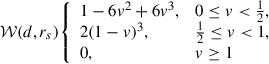
![Mathematical equation: $$ \begin{aligned}&f(d,h_s) \nonumber \\&\frac{1}{h_s}{\left\{ \begin{array}{ll} \left(-\frac{16}{3}v^{{\prime }2} + \frac{48}{5}v^{{\prime }4} -\frac{32}{5}v^{{\prime }5} + \frac{14}{5}\right),&\mathrm{if}\; 0 \le v^{\prime } < \frac{1}{2}.\\ [2mm] \left(\frac{-1}{15v^{\prime }} - \frac{32}{3}v^{{\prime }2} +16v^{{\prime }3} - \frac{48}{5}v^{{\prime }4} + \frac{32}{15}v^{{\prime }5} + \frac{16}{5}\right),&\mathrm{if}\; \frac{1}{2} \le v^{\prime } < 1.\\ [2mm] \frac{1}{v^{\prime }},&\mathrm{if}\; v^{\prime } \ge 1. \end{array}\right.} \end{aligned} $$](/articles/aa/full_html/2026/03/aa58057-25/aa58057-25-eq11.gif) (8)
(8)
Here, v′≔d/hs and hs is the gravitational softening radius. In this work, we set rs = hs.
Our simulations are susceptible to numerical shock instabilities when multidimensional shocks align with the grid, often triggering the carbuncle phenomenon, where odd-even perturbations grow unphysically (Quirk 1994). To mitigate this, we employed the low-dissipation Harten-Lax-van Leer Riemann solver (LHLLC; Minoshima & Miyoshi 2021)1, which introduces targeted tangential dissipation to suppress such perturbations. Spatial reconstruction of the primitive variables is performed using the piecewise parabolic method (Colella & Sekora 2008). We disabled the extremum-preserving limiters to improve numerical stability, particularly near the gravitational potential minimum. Time integration uses a strong-stability-preserving third-order Runge-Kutta method (Shu & Osher 1988; Gottlieb et al. 2009).
2.2. Initial conditions
2.2.1. Stratified case
As in Gagnier & Pejcha (2023, 2024, 2025), we initialized the envelope of the primary star in hydrostatic equilibrium with purely radial density and pressure profiles following a polytropic relation with polytropic index n = 1/(Γ − 1). The gas obeys an ideal-gas equation of state, and gas self-gravity is neglected. Doing so, the local stellar structure around r = r2, for a binary with a mass ratio q = M2/M1, can be characterized with two parameters: the density at r = r2 and the ratio between the Hoyle–Lyttleton radius and density scale-height at the same location:
 (9)
(9)
with
 (10)
(10)
and where u∞ = r2Ω is the companion’s orbital velocity. We further express the Bondi–Hoyle–Lyttleton radius as
 (11)
(11)
where cs, ∞ = cs(r2, t = 0) is the sound speed of the unperturbed envelope at the companion’s location. Using the hydrostatic equilibrium equation, one can derive the density and pressure profiles:
![Mathematical equation: $$ \begin{aligned} \rho (r)&= \left[\frac{(1-\Gamma )GM_1}{K\Gamma } \left(\frac{2q}{(1+q)R_a} \left(1+\frac{2q}{\epsilon _\rho (1+q)(1-\Gamma )}\right) - \frac{1}{r}\right)\right]^n, \end{aligned} $$](/articles/aa/full_html/2026/03/aa58057-25/aa58057-25-eq15.gif) (12)
(12)
 (13)
(13)
where
 (14)
(14)
Equations (1a), (1b), and (1c) are homogeneous in density. Varying ρ(r2) therefore does not change the flow structure or the normalized drag, lift, and accretion coefficients (Sect. 2.4), but only their absolute values. The 2 M⊙ red giant MESA model shown in Fig. 1 illustrates how the stratification parameter (ϵρ) varies across a realistic envelope and provides a reference for assessing the accuracy of our local polytropic reconstruction. The simulation results presented in this paper are expressed in terms of dimensionless parameters and are therefore not tied to this particular stellar model.
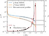 |
Fig. 1. Density and pressure profiles from the 2 M⊙ red giant MESA model of Ohlmann et al. (2016), shown as a function of the radius. Dashed lines indicate the polytropic reconstruction used as initial conditions, computed around the location where ϵρ = 3, which is marked by red crosses. The vertical line marks the radius where ϵρ = 10 in the reconstructed stellar structure. The red curve shows the stratification parameter (ϵρ) as a function of radius for the MESA model, while black dots indicate the ϵρ values employed in our simulations. |
In order to minimize the effects of the non-exact numerical hydrostatic equilibrium resulting from the finite grid resolution, we used Gauss-Legendre quadrature of order 12 to map the initial profiles onto the mesh as volume-averaged variables at the barycenter of each cell, which is different from geometric center in polar-spherical coordinates. The initial velocity of the gas in the companion’s orbiting frame is set to U = r sin θΩeφ at t = 0, so that the envelope is initially nonrotating in the inertial frame. Crucially, unlike in wind-tunnel simulations, the primary’s envelope in our setup is in hydrostatic equilibrium in the absence of the companion.
In our stratified simulations, the domain size is such that it accommodates a sphere of radius  , so that the radial extent of the domain is
  , and its angular extent is
 (15)
(15)
where we have set φ2 = 0 and θ2 = π/2. We chose a mass ratio q = 0.1 so that  and the domain does not include the primary’s core. In regimes of strong stratification (ϵρ ≳ 1), the outer radial boundary of the computational domain can extend beyond the stellar surface, requiring the modeling of an outer vacuum-like atmosphere (e.g., MacLeod et al. 2018; Gagnier & Pejcha 2023). To handle this, we defined a critical radius (rc) at which the transition from the stellar envelope to the atmosphere occurs. In this work, we set rc to be the radius at which the local stratification parameter of the reconstructed profile reaches a value of 10, coinciding approximately with both the maximum of ϵρ and the location of the stellar surface in the one-dimensional MESA model (see Fig. 1). The atmosphere is assumed to be isothermal and in hydrostatic equilibrium, and it is smoothly matched to the envelope by ensuring continuity of the density, pressure, and pressure gradient at r = rc. The resulting atmospheric density and pressure profiles are given by
![Mathematical equation: $$ \begin{aligned} \rho (r \ge r_c)&= \rho (r_c) \exp \left[\frac{\Gamma GM_1}{(c^a_s)^2} \left(\frac{1}{r} - \frac{1}{r_c}\right)\right], \end{aligned} $$](/articles/aa/full_html/2026/03/aa58057-25/aa58057-25-eq22.gif) (16)
(16)
 (17)
(17)
where the atmosphere’s sound speed is defined as  .
.
2.2.2. Non-stratified case
For the non-stratified simulations presented in Sects. 3.1, 3.2, and 3.3, we set M2 = 1, Φ1 = 0, Ra = 1, ρ(t = 0) = 1, and thus  . The initial gas pressure is set by choosing the Mach number, P(t = 0) = u∞2/(ℳ∞2Γ). The companion’s position with respect to the center of rotation is r2 = Ro Ra where the Rossby number Ro is prescribed, and the orbital angular velocity therefore reads Ω = u∞/r2. In the nonrotating wind-tunnel simulations, we set the wind velocity U = u∞.
2.3. Mesh structure and boundary conditions
Our root-level grid resolution is 2563, on top of which we added four levels of adaptive mesh refinement. We adopted a mesh refinement criterion based on the second derivative error norm of a function σ (Lohner et al. 1987). A mesh block is tagged for refinement whenever the following condition is met for a given number of successive cycles (e.g., Mignone et al. 2012; Gagnier & Pejcha 2023):
 (18)
(18)
where, for instance, Δr, ±1/2σ = ±(σi ± 1 − σi) and σr, ref = |σi + 1|+2|σi|+|σi − 1|. The parameter ϵ is introduced as a filter to prevent refinement in regions with small-scale fluctuations or noise, and we typically set ϵ = 0.01. In our simulations, we used σ = ℳ = |u|/cs and χr′=χr + b(1 − χr), where χr = 0.95. Here, b is defined as the minimum of 1 and the ratio of the total number of 163-cell mesh blocks to a user-specified maximum, which we set to 105. In quasi-steady state, each simulation contains approximately 4.1 × 10⁸ cells. A mesh block is tagged for de-refinement whenever χ < χd − b(1 − χd), with χd = 0.8, for 20 successive cycles. We imposed no-inflow boundary conditions at both radial boundaries and at the minimum-φ boundary, and outflow boundary conditions at both θ boundaries. Pressure and density in the ghost cells at the inner radial boundary and at the maximum-φ boundary follow Eqs. (12) and (13), with the azimuthal velocity in the ghost cells at the maximum-φ boundary set to U. Quantities in the ghost cells at the maximum-φ boundary are evaluated using Gauss-Legendre quadrature.
2.4. Diagnostics
In this section we summarize the diagnostics computed at runtime in our simulations.
2.4.1. Accreted quantities
The total mass accretion rate onto the sink particle is
 (19)
(19)
The spin torque, associated with the change in the sink’s internal angular momentum, is
 (20)
(20)
Here, δ = 0 corresponds to neglecting the spin torque. The linear momentum transfer rate in the direction i due to accretion is
 (21)
(21)
2.4.2. Drag and lift forces
The drag force, integrated within a sphere of radius Ri of volume Vi around the companion, is
 (22)
(22)
Similarly, the radial (lift) force, integrated within the same volume, is
 (23)
(23)
In this work, we neglected the hydrodynamic drag and lift forces, as they are expected to be orders of magnitude weaker than their gravitational counterparts (e.g., Ricker & Taam 2012), with Fhydro/Fdrag ∼ (R2/Ra)2 ≪ 1, where R2 is the radius of the companion.
3. Results
3.1. Nonrotating, non-stratified, and non-accreting case
As a fiducial model, we considered wind-tunnel simulations in which a uniform supersonic flow impinges on a non-accreting point mass, similar to the setups of Thun et al. (2016) and Prust & Bildsten (2024). In our case, however, the companion is neither a solid sphere nor an absorbing boundary, but instead is represented by a softened gravitational potential. This is the same treatment used for the companion and the primary’s core in global common-envelope simulations. Our local, high-resolution models allow us to resolve the small-scale flow around the companion. For a companion star of radius R2, the degree of flow nonlinearity can be quantified by the parameter (Kim & Kim 2009)
 (24)
(24)
where ℳ∞ = ℳ(r2, t = 0) is the Mach number of the companion in the unperturbed envelope. Prust & Bildsten (2024) show that when η ≫ 1, a hydrostatic halo forms around the companion. In our setup, R2 → 0 and thus η → ∞. We therefore expect the formation of a hydrostatic bubble, analogous to the halos reported in Thun et al. (2016) and Prust & Bildsten (2024). Assuming such a bubble exists and extends up to the shock front, its density and pressure profiles follow directly from hydrostatic equilibrium:
![Mathematical equation: $$ \begin{aligned} \rho (d)&= \rho (d_s) \left[1 - \frac{\Gamma - 1}{c_{s,\mathrm{ps}}^2} \left(\Phi _2 - \Phi _2(d_s)\right)\right]^n, \end{aligned} $$](/articles/aa/full_html/2026/03/aa58057-25/aa58057-25-eq33.gif) (25)
(25)
 (26)
(26)
Here
 (27)
(27)
is the shock stand-off distance, with κ a factor of order unity (Thun et al. 2016), which we set to 1, and
![Mathematical equation: $$ \begin{aligned} K_2 = \frac{P_{\infty }}{\rho _{\infty }^{\Gamma }} \frac{\left[(\Gamma - 1)(3 {\mathcal{M} }_{\infty }^{2} - 2) + 2 \right]^{\Gamma } \left[(\Gamma + 1) + 6 \Gamma ({\mathcal{M} }_{\infty }^{2} - 1)\right]}{\left[(\Gamma + 1)(3 {\mathcal{M} }_{\infty }^{2} - 2)\right]^{\Gamma }}, \end{aligned} $$](/articles/aa/full_html/2026/03/aa58057-25/aa58057-25-eq36.gif) (28)
(28)
where ρ∞ and P∞ are respectively the density and pressure of the unperturbed envelope at the companion’s location. Using the Rankine–Hugoniot conditions together with pre-shock energy conservation, u∞2/2 = ups2/2 − GM/ds, the post-shock sound speed is cs, ps2 = cs, ∞2 ξ(ℳ∞, Γ), where
 (29)
(29)
Figure 2 compares these analytical density and pressure profiles with results from a nonrotating, non-stratified, and non-accreting wind-tunnel simulation with ℳ∞ ≔ u∞/cs, ∞ = 4, and hs = 0.05 Ra. Profiles are shown along the six Cartesian radial directions centered on the companion (±x, ±y, ±z), within the xy and xz planes. The comparison shows excellent agreement: both the analytical profiles and the predicted shock location from Eq. (27) reproduce the simulation results with high accuracy. This indicates that a quasi-hydrostatic bubble indeed forms around the point mass and extends out to the shock front. To assess whether this bubble is energetically bound or unbound, we evaluated the Bernoulli parameter:
 (30)
(30)
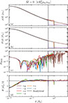 |
Fig. 2. Density (panel a), pressure (panel b), normalized hydrostatic balance residual RHSE = ∥∇P+ρ ∇Φ2∥/max(∥∇P∥, ∥ρ ∇Φ2∥) (panel c), and Bernoulli parameter (panel d) profiles along radial rays from the companion for a nonrotating, non-stratified, and non-accreting simulation with ℳ∞ = 4. Gray lines indicate the analytical solutions for density and pressure (Eqs. 25, 26) and the hydrostatic Bernoulli parameter ℬHSE (Eq. 31). The vertical dashed line marks the predicted shock radius, ds (Eq. 27). All quantities are averaged over a duration of Δt = Ra/u∞ once a quasi-steady state has been reached. |
where h = (P + e)/ρ is the specific enthalpy. By definition, within the quasi-hydrostatic bubble, ∥u∥≃0 and ∂dℬ ≃ 0, so
 (31)
(31)
Thus, the condition for the gas bubble to be formally gravitationally bound (ℬHSE ≤ 0) reduces to a simple inequality involving only Γ and ℳ∞:
 (32)
(32)
For adiabatic indices relevant to stellar interiors(1 < Γ < 5/3), condition (32) is never satisfied for supersonic flows (ℳ∞ ≥ 1). In other words, no formally gravitationally bound hydrostatic bubble can form around a point mass in the standard wind-tunnel setup. The gas is energetically unbound, so local perturbations at the bubble’s surface, such as turbulence or small density fluctuations, could in principle trigger expansion and allow some material to escape. In practice, however, the shock upstream and the continuous inflow downstream act to confine the gas, maintaining a quasi-stable hydrostatic bubble around the point mass. We verified the theoretical Bernoulli parameter in the post-shock region (31) as well as the hydrostatic balance residual in Fig. 2. Good agreement is found except very close to the point mass, where h + Φ2 ≪ |h|∼|Φ2|. In this region, even small errors δh arising from finite resolution or the non-spherically symmetric grid around the companion lead to large fractional deviations in the Bernoulli parameter, δℬ/|ℬ|=δh/|ℬ|≫1.
In a uniform gaseous medium, the gravitational drag exerted on a supersonically moving point mass is expected to grow logarithmically with the integration radius (Ruderman & Spiegel 1971),
 (33)
(33)
where bmax is the radius of integration, and bmin is the effective inner cutoff for which the linear theory underlying the Coulomb-logarithm scaling Eq. (33) remains valid. What sets this cutoff has been discussed extensively in the literature. Often, either the physical radius (R) of the object or (for a compact and massive body) bmin ≃ max(R, Ra) is chosen. Thun et al. (2016) identify bmin with the shock standoff distance ds (Eq. 27), effectively treating it as the minimum spatial scale of interaction below which gas exerts no drag. This interpretation is misleading as bmin is not the scale at which the drag vanishes, but rather the smallest radius where the linear Coulomb-logarithm scaling applies. Gas inside bmin still exerts force, but its contribution does not follow the logarithmic scaling. In Fig. A.1 we show the time evolution of the gravitational drag measured within different logarithmically spaced integration radii, scaled by the Coulomb logarithm. In a quasi-steady state, the curves are consistent with the Coulomb-logarithm scaling for an effective inner cutoff of bmin ≃ 0.78 Ra, about 50% larger than the shock standoff distance ds. In an infinite uniform medium, the drag force would formally diverge, but in practice bmax is limited by the causal extent of the wake, u∞t. At t = 200 Ra/u∞, this corresponds to bmax ≃ 200 Ra, implying that the gravitational drag enclosed within our numerical domain represents only ∼24% of the total drag force at that time. This may become a significant limitation for local simulations or global simulations with a limited numerical domain size. Indeed, including stratification, magnetic fields, or accretion may cause the drag force to deviate from a simple Coulomb-logarithm scaling. In such cases, the limited domain may prevent the development of reliable drag force prescriptions (see also Sect. 3.4.2).
3.2. Accretion effects
While jet-like outflows are observed in hydrodynamical simulations of CEE (Gagnier & Pejcha 2025; Lau et al. 2025), the high-momentum outflows observed in protoplanetary nebulae and planetary nebulae likely require additional energy transfer such as magnetic energy conversion via Lorentz force (Ondratschek et al. 2022; Gagnier & Pejcha 2024; Vetter et al. 2024, 2025) or accretion onto the companion (Ricker & Taam 2012; Blackman & Lucchini 2014; Chamandy et al. 2018). To investigate the latter, we used the simplified wind-tunnel setup described above but allowed the companion to accrete mass, momentum, and energy.
In Fig. A.2 we show density, pressure, normalized hydrostatic balance residual, and Bernoulli parameter profiles along radial rays from the companion for a simulation run with hs = 0.05 Ra, ℳ∞ = 4, δ = 0, and γ = 100. In a quasi-steady state, this corresponds to an accretion rate Ṁ ≃ 0.02 ṀHL, where  is the Hoyle–Lyttleton accretion rate (Hoyle & Lyttleton 1939). Although such an accretion rate is far below the Hoyle–Lyttleton prediction, its associated inflow is sufficient to destabilize the gas near the companion. Instead of accumulating into a quasi-hydrostatic, pressure-supported bubble, material is continuously drained and funneled through the asymmetric wake. This sustained inflow creates strong velocity shear near the companion, driving turbulence and inducing collisions between converging streams. Accretion contributes to local vorticity through the sink term
  , which vanishes only when
  . Additional vorticity is generated by departures from hydrostatic equilibrium and accretion anisotropies (mostly resulting from rotation and/or stratification; see Sects. 3.3 and 3.4), via the baroclinic torque, (∇ρ × ∇P)/ρ2. Collisions between converging streams then produce weak shocks and small-scale viscous dissipation that locally increase the entropy2. The higher-entropy gas is advected downstream, where it expands and forms bubble-like structures in the wake, while simultaneously perturbing the upstream flow and distorting the bow shock, causing the standoff distance to fluctuate. This is illustrated in Fig. 3, where we show density, pseudo-entropy, and Mach number snapshots taken at t = 100 Ra/u∞, for the two aforementioned simulations.
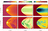 |
Fig. 3. Zoomed-in snapshots in the xy plane of the density, pseudo-entropy, and Mach number at t = 100 Ra/u∞ for non-stratified simulations with hs = 0.05 Ra and ℳ∞ = 4. First row: Non-accreting case. Second row: Accreting case with γ = 100 and δ = 0. |
Such turbulent, anisotropic accretion-driven flows may efficiently amplify magnetic fields through stretching, twisting, and folding of field lines, potentially producing much faster magnetic energy growth near the companion than in the non-accreting regime. Even without accretion, magnetic fields can significantly influence the binary separation evolution, drive jet-like outflows (Ondratschek et al. 2022; Vetter et al. 2024, 2025), and contribute to angular momentum transport during the post-dynamical phase (Gagnier & Pejcha 2024). Accretion may therefore further strengthen the magnetic feedback on the system. These effects will be explored in detail in a forthcoming work (Gagnier et al., in prep.). Figure 4 shows the time evolution of the drag and radial forces acting on the companion, for a non-accreting simulation as well as accreting simulations with γ = 100 and δ = 0 and 1. We find that, while accretion induces strong temporal variability in both drag and radial forces, the resulting change in the mean drag force is likely not significant in view of the system’s intrinsic stochastic fluctuations (see Appendix B). These force fluctuations translate directly into variations in the companion’s instantaneous orbital decay rate, while the variable balance between drag and radial forces can excite eccentricity during the dynamical inspiral. The impact of both effects on the orbital evolution remains to be quantified. For clarity, the linear momentum accretion rate is omitted from the figure. It acts like a small “negative” drag force (or thrust), contributing only ∼0.27% of the drag for δ = 0 and ∼0.55% for δ = 1.
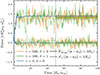 |
Fig. 4. Time evolution of the radial and drag forces exerted by the gas on the companion in non-stratified simulations with Ro = 5.5 and ℳ∞ = 4, with and without accretion. Forces are integrated within a sphere of radius 3 Ra. The shaded regions indicate the 3σ range (see Appendix B). |
3.3. Rotational effects
The Rossby number,
 (34)
(34)
quantifies the dynamical importance of rotation in the flow. For typical common-envelope parameters, with a binary mass ratio q = 0.1 and a stratification parameter ϵρ = 𝒪(1), Ro = 𝒪(1). This implies that rotational effects associated with the orbital motion cannot be neglected. Still, standard wind-tunnel simulations (e.g., MacLeod & Ramirez-Ruiz 2015; Thun et al. 2016; MacLeod et al. 2017; De et al. 2020; Prust & Bildsten 2024) ignore rotation entirely.
Rotation breaks the mirror symmetry of the flow, both dynamically via the Coriolis force and statically through the asymmetry of the effective gravito-centrifugal potential, Φgc = Φ1 + Φ2 − (Ωez × r)2/2. In the orbiting frame with angular velocity Ω, the azimuthal velocity of the inflowing gas increases linearly with distance from the rotation axis, further enhancing the symmetry breaking. As a result of this broken symmetry, inflowing material is deflected around the companion, generating z-directed angular momentum in the companion frame and producing a net positive lift force. This effect is illustrated in Fig. 5, where we compare density snapshots from a Cartesian wind-tunnel and a rotating simulation on a spherical grid with Ro = 5.5, at quasi-steady state. Both simulations are non-stratified, non-accreting, and have ℳ∞ = 2 and hs = 0.1, Ra. Figure 6 shows the time evolution of the drag and lift forces. While rotation only slightly increases the drag force (by ∼14% in this example), the lift force may significantly influence orbital contraction and excite eccentricity during the plunge-in phase (see also Sect. 3.4.2). The flow also develops a secondary shock and strong, large-scale shear, which triggers shear instabilities that drive turbulent eddies. Numerical dissipation of these eddies generates entropy, heating the gas and driving the expansion of hot bubbles.
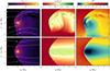 |
Fig. 5. Zoomed-in density, pseudo-entropy, and Mach number snapshots at t = 100 Ra/u∞ in the xy plane for non-stratified simulations with Ro = 5.5 and ℳ∞ = 2. The top panel includes rotation; the bottom does not. White lines indicate streamlines. |
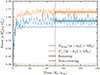 |
Fig. 6. Time evolution of the radial and drag forces exerted by the gas on the companion in non-stratified simulations with Ro = 5.5 and ℳ∞ = 2, with and without rotation. Forces are integrated within a sphere of radius 3Ra. The shaded regions indicate the 3σ range (see Appendix B). |
3.4. Stratification effects
We performed hydrodynamical simulations with a fixed softening radius of  . Unlike the previous sections, which focus on unstratified envelopes, we now explore the effects of stratification by varying the parameter ϵρ, thereby probing different depths within the primary’s envelope (see Fig. 1). In these stratified runs, the Mach number of the flow is directly determined by the value of ϵρ:
 (35)
(35)
3.4.1. Flow morphology
Figure 7 shows zoomed-in snapshots of density at  , in the xy orbital plane and projected on a spherical shell at radius r2, for different values of the stratification parameter (ϵρ), including rotation but without accretion. Here, ϵρ = 0.2 corresponds to the innermost part of the 2 M⊙ red giant envelope, while ϵρ = 10 corresponds to the outermost parts (see Fig. 1). In these simulations, the upstream flow is vertically stratified in density and pressure, and the local Mach number varies vertically due to the combined effects of the radial sound-speed gradient from stratification and the azimuthal velocity profile with constant angular velocity Ω. The companion gravitationally deflects the surrounding gas, and the density stratification produces asymmetric gravitational focusing, with denser layers contributing more inertia, resulting in a vertically offset wake. Coriolis and centrifugal forces in the rotating frame further influence the vertical asymmetry of the wake (see Sect. 3.3). The magnitude of the mirror asymmetry increases with the stratification parameter (ϵρ). The post-shock radial stratification is shaped by the upstream density and pressure structure and the radial variation of the upstream velocity. This results in a corresponding radial variation in post-shock azimuthal momentum, which causes the gas to be differentially deflected by the companion and generates z-directed angular momentum in the companion’s orbiting frame (
 ). For ϵρ ≳ 3, strong shear flows develop around the companion in the orbital plane and in the wake above and below it, leading to Kelvin-Helmholtz instabilities.
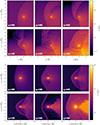 |
Fig. 7. Zoomed-in snapshots of the density at |

3.4.2. Drag and lift forces
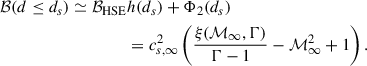
Figure 8 shows the time-averaged drag and radial forces exerted by the gas on the companion, averaged over ![Mathematical equation: $ t \in [50,\,100]\,\widetilde{R_a}/u_{\infty} $](/articles/aa/full_html/2026/03/aa58057-25/aa58057-25-eq51.gif) as functions of the stratification parameter (ϵρ) and of the radius of the integration volume. Similar to MacLeod et al. (2017) and De et al. (2020), we find that the drag force increases with increasing stratification strength. The fitting formula for the drag force proposed by De et al. (2020) provides an excellent match to our results in strongly stratified parts of the envelope (ϵρ > 0.7), but significantly overestimates the drag in more weakly stratified regions. This difference arises because our simulations neglect accretion, so the measured drag reflects only the gravitational interaction with the stratified gas. In contrast, MacLeod et al. (2017) and De et al. (2020) remove mass over a large region around the companion, transferring momentum from the gas to the object. While this mass removal generally reduces the net drag force (e.g., MacLeod et al. 2017, and Sect. 3.5), it also alters the large-scale density distribution, which can increase the total measured drag force. In strongly stratified flows, the accretion rate is lower (see Fig. A.3 and Sect. 3.5), and the steep density gradients dominate the wake structure, reducing the discrepancy between the two approaches. By neglecting accretion, we isolate the drag arising solely from the gravitational interaction with the stratified gas, without relying on sub-grid accretion prescriptions. Accretion effects are discussed separately in Sects. 3.2 and 3.5. For q = 0.1, we provide an alternative fitting formula for the gravitational drag force in Eq. (36).
as functions of the stratification parameter (ϵρ) and of the radius of the integration volume. Similar to MacLeod et al. (2017) and De et al. (2020), we find that the drag force increases with increasing stratification strength. The fitting formula for the drag force proposed by De et al. (2020) provides an excellent match to our results in strongly stratified parts of the envelope (ϵρ > 0.7), but significantly overestimates the drag in more weakly stratified regions. This difference arises because our simulations neglect accretion, so the measured drag reflects only the gravitational interaction with the stratified gas. In contrast, MacLeod et al. (2017) and De et al. (2020) remove mass over a large region around the companion, transferring momentum from the gas to the object. While this mass removal generally reduces the net drag force (e.g., MacLeod et al. 2017, and Sect. 3.5), it also alters the large-scale density distribution, which can increase the total measured drag force. In strongly stratified flows, the accretion rate is lower (see Fig. A.3 and Sect. 3.5), and the steep density gradients dominate the wake structure, reducing the discrepancy between the two approaches. By neglecting accretion, we isolate the drag arising solely from the gravitational interaction with the stratified gas, without relying on sub-grid accretion prescriptions. Accretion effects are discussed separately in Sects. 3.2 and 3.5. For q = 0.1, we provide an alternative fitting formula for the gravitational drag force in Eq. (36).
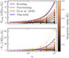 |
Fig. 8. Time-averaged drag (top) and lift (bottom) forces on the companion as functions of the stratification parameter (ϵρ) and integration radius, averaged over |
![Mathematical equation: $ t \in [50,\,100]\,\widetilde{R_a}/u_{\infty} $](/articles/aa/full_html/2026/03/aa58057-25/aa58057-25-eq52.gif)
Stratification also generates a lift force perpendicular to the companion’s orbital motion. For steep density gradients, this force is directed inward, toward higher-density regions, and its magnitude increases with both ϵρ and the size of the integration volume. However, for weak stratification (ϵρ ≲ 0.5), the lift force reverses direction, producing a net outward contribution that remains too small to significantly affect the orbital evolution. As discussed in Sect. 3.3, rotation has the opposite effect: it generates an outward force, directed toward lower-density regions. Including rotation therefore reduces the net inward force, especially in outer layers with high ϵρ and thus low Ro. This is illustrated in the bottom panel of Fig. 8. For a binary mass ratio q = 0.1, we propose a simple fitting formula for this lift force in Eq. (36b).
 (36)
(36)
 (36b)
(36b)
where  . Fitting coefficients am and bm are given in Table A.1. Convergence tests for ϵρ = 3 (Fig. A.4) show that both drag and lift forces converge for softening radii below roughly
  . The value used in this section,
  , falls well within the converged regime. We expect this behavior to hold for other values of ϵρ. We show the solution to a two-body problem that includes drag and lift forces acting on the secondary in Fig. A.5. For that, we used the ϵρ radial profile of the 2 M⊙ red giant MESA profile (Fig. 1), and we assumed a mass ratio q = 0.1. The secondary star is subject to the gravity force from the enclosed primary mass and experiences additional drag and lift forces. We compared four models: (1) our full prescription with drag and lift forces (Eqs. 36 and 36b); (2) the same, but with F⊥ = 0; (3) the drag force prescription from De et al. (2020); and (4) a standard Hoyle–Lyttleton drag force πRa2ρ∞u∞2. We find that our model (Eqs. 36 and 36b) results in an initial inspiral that is faster than both the standard Hoyle–Lyttleton drag and the drag force prescription from De et al. (2020). In the outer layers, where ϵρ > 0.7, the difference with De et al. (2020) arises from the inclusion of the (inward) lift force F⊥. In the innermost layers, where stratification is weaker (ϵρ < 0.7), further differences stem from the stronger drag force in our model.
As in the non-stratified simulations, we find that the drag force follows the Coulomb-logarithm scaling (33), but with  , and only for integration radii
  . Consequently, the fitting formula for the drag force (36) can be rescaled for larger radii
  by
by
 (37)
(37)
keeping in mind that bmax is bound by the causal extent of the wake. Conversely, the lift force does not follow a Coulomb-logarithm scaling, and its dependence on bmax varies with the stratification parameter, precluding a simple rescaling. Consequently, Eq. (36b) should be regarded as a lower bound for the actual lift force acting on the companion. This limitation complicates the ability of local simulations to accurately capture its role in orbital evolution and eccentricity excitation, and poses a challenge for devising reliable prescriptions for one-dimensional evolutionary codes.
3.5. Combined effects of stratification, rotation, and accretion
Here, we investigate the combined effects of stratification, rotation, and accretion. We consider three stratification parameters, ϵρ = 0.3, 0.5, and 3, which correspond approximately to r2/R* ≃ 0.35, 0.5, and 0.9, respectively. In this section, unless stated otherwise, we adopt γ = 1000 and δ = 1, yielding mass accretion rates (in terms of ṀHL) comparable to those of the non-stratified simulations with γ = 100 presented in Sect. 3.2. The parameters and diagnostics of these simulations are summarized in Table A.2.
Figure 9 shows the normalized hydrostatic-centrifugal balance residual profiles along radial rays from the companion for a non-accreting and an accreting simulation with ϵρ = 3, averaged over ![Mathematical equation: $ t \in [99, 100]\,\widetilde{R_a}/u_{\infty} $](/articles/aa/full_html/2026/03/aa58057-25/aa58057-25-eq62.gif) . As also found in Sect. 3.2, accretion prevents the formation of a quasi-hydrostatic bubble around the companion (see also Figs. A.6 and A.7). In the absence of accretion, such a bubble forms, with the centrifugal contribution to the force balance being less than 10% of the gravitational force (not shown). Unlike the non-stratified, nonrotating case, the bubble does not extend to the shock front and instead has a radius of
. As also found in Sect. 3.2, accretion prevents the formation of a quasi-hydrostatic bubble around the companion (see also Figs. A.6 and A.7). In the absence of accretion, such a bubble forms, with the centrifugal contribution to the force balance being less than 10% of the gravitational force (not shown). Unlike the non-stratified, nonrotating case, the bubble does not extend to the shock front and instead has a radius of  . Quasi-hydrostatic equilibrium implies barotropicity and thus an absence of vorticity generation from baroclinic torque within the bubble.
 |
Fig. 9. Normalized hydrostatic-centrifugal balance residual |

![Mathematical equation: $ t \in [99, 100]\,\widetilde{R_a}/u_{\infty} $](/articles/aa/full_html/2026/03/aa58057-25/aa58057-25-eq65.gif)
We verified that the radius of the quasi-hydrostatic bubble does not depend on the softening radius in the non-accreting simulation by repeating it with hs = 0.1, 0.2, and  . The bubble size remains unchanged for
  , but it does not form for
  . Increasing the softening radius weakens the hydrostatic support of the gas surrounding the companion, making it more susceptible to perturbations from the strong surrounding flow (Gagnier & Pejcha 2025). This same strong rotational flow also limits the extent of the hydrostatic bubble to a fraction of the shock stand-off distance. By contrast, in the accreting case, the gas near the companion is baroclinic (see Fig. A.8), leading to vorticity generation that may enhance local magnetic field amplification, compared to non-accreting simulations. The same behavior is observed for both ϵρ = 0.3 and 0.5. In these cases, however, the stratification-induced asymmetry is much smaller than for ϵρ = 3, resulting in weaker z-directed angular momentum in the companion frame. This results in reduced shear and turbulence, leading to a more stable flow in the companion’s vicinity. In the absence of accretion, the quasi-hydrostatic bubble is therefore significantly larger for weaker envelope stratification. In particular, for both ϵρ = 0.3 and 0.5, the bubble extends all the way to the shock front, similarly to the non-stratified and nonrotating simulations discussed in Sect. 3.2. We did not investigate the dependence of the bubble size on the softening radius for the stratification parameters considered here.
Despite accretion’s impact on turbulence, the drag and lift forces remain essentially unchanged (see Table A.2). Still, accretion plays a crucial thermodynamic role. The inflow generates entropy through shocks and small-scale dissipation near the companion (e.g., Figs. A.6 and A.7), converting a fraction of the orbital energy into thermal energy. This heating is then advected downstream, contributing to the gravitational unbinding of the envelope.
We further find that the contribution of linear momentum accretion to the total drag force increases as the stratification parameter (ϵρ) decreases and appears to saturate in the weak-stratification regime (see Table A.2). Additional simulations are required to confirm this trend. The main reason for this increase toward lower ϵρ is that regions with smaller stratification parameters correspond to denser parts of the envelope, where accretion rates are higher. A similar trend is observed for the radial force; however, it does not saturate in the asymptotic limit of weak stratification, since both the radial momentum accretion and the lift force should vanish as ϵρ → 0. Indeed, in this limit, the Rossby number diverges and the combined effects of stratification and rotation on wake asymmetry disappear, yielding  and F⊥ → 0. For finite ϵρ, linear momentum accretion remains finite, producing a net thrust and lift force.
We finally briefly investigated the effect of allowing angular momentum accretion onto the companion’s spin by choosing δ = 1. To this end, we assumed the companion to be a 0.2 M⊙ white dwarf (WD) with a radius R2 ∼ 0.02 R⊙3. The specific angular momentum of the accreted material along the companion’s z-axis reads
 (38)
(38)
We report this quantity normalized by the Keplerian value at the WD surface  in Table A.2. As expected from the increasing wake asymmetry with stronger stratification, ℓz increases with increasing ϵρ. For ϵρ = 3, ℓz is ∼80% of the Keplerian value at the WD surface. Because ℓz is computed from the total angular momentum and mass accretion rates integrated over the sink region, it represents a weighted average over the accreted material. Hence, for ϵρ = 3, individual parcels of accreted gas can already carry specific angular momentum above the Keplerian value. At larger ϵρ, i.e., closer to the stellar surface, the global ℓz itself is expected to exceed the Keplerian limit. These results indicate that, even though the corresponding accretion rate is only about 1% of the Hoyle–Lyttleton rate, the combination of parameters γ = 1000 and δ = 1 likely overestimates the spin torque on the WD. Assuming uniform rotation of the WD, as well as a radius of gyration k = 0.2 (Andronov & Yavorskij 1990), we can measure the corresponding spin-up timescale,
 (39)
(39)
The values of τspin − up are also reported in Table A.2. We find that for all three accreting simulations, even in the ϵρ = 3 case where part of the accreted material is likely rotating super-critically, the spin-up timescale of the WD remains much longer than the dynamical inspiral timescale, which is of order 1 Porb. This suggests that the WD’s spin is unlikely to change significantly during the dynamical inspiral phase. Moreover, we find that the dependence of τspin − up on ϵρ is non-monotonic. This behavior arises because τspin−up ∝ (ℓz M⊙)−1, with ℓz increasing with ϵρ while Ṁ decreases with increasing ϵρ. This suggests the existence of a critical stratification parameter 0.5 ≲ ϵρc ≲ 3 at which the spin-up timescale reaches a minimum for our specific simulations parameters. We finally note that magnetic torques could modify the spin-up timescale by transferring angular momentum between the WD and the surrounding material.
4. Conclusion
We studied the effects of rotation, accretion, and stratification on the dynamical inspiral phase of CEE. To this end, we performed three-dimensional local simulations of a 0.2 M⊙ compact companion plunging into the envelope of a 2 M⊙ red giant in the companion’s orbiting frame, using the Athena++ code. Accretion onto the companion was modeled with either a standard sink, which allows angular momentum accretion onto the companion’s spin, or a torque-free sink, which prevents it. The main results are as follows:
-
The rotation associated with the orbital motion has a weak impact on the gravitational drag force. Measured drag forces are consistent with De et al. (2020) in the strong stratification regime. Asymmetries from the Coriolis force and the effective gravito-centrifugal potential generate a lift force, which partially counteracts the inward radial force from density stratification. The total radial force significantly affects the orbital evolution and cannot be neglected. We propose a new prescription for both drag and lift forces. Unlike the drag, the lift force does not follow a Coulomb-logarithm scaling, and the proposed lift force prescription should therefore be regarded as a lower limit.
-
In the absence of accretion, a quasi-hydrostatic bubble forms around the companion. In the weak stratification regime, the bubble extends up to the shock front, while in the strong stratification regime, strong rotational flows in the companion’s frame limit its radius. Such bubbles contribute negligibly to the net drag and lift forces and suppress vorticity growth. In the non-stratified and nonrotating regime, the bubble is never formally gravitationally bound and can be disrupted by small perturbations.
-
Accretion prevents the formation of a quasi-hydrostatic bubble, producing weak shocks and strong turbulence near the companion. These processes generate entropy that is advected downstream and may aid envelope ejection and enhance magnetic energy amplification. Within the considered parameter space, accretion marginally affects drag and lift forces, remaining within the intrinsic stochastic variability of the flow. Using a standard sink, angular momentum accretion onto the companion’s spin can be overestimated because the companion’s physical size is much smaller than the sink radius. The companion’s spin-up timescale remains much longer than the dynamical inspiral timescale. The spin-up rate varies non-monotonically with depth, peaking at intermediate radii where the product of accreted specific angular momentum, ℓz, and accretion rate, Ṁ, is largest.
Magnetic fields influence CEE by affecting gas dynamics and orbital separation and contributing to the launching of bipolar outflows (Ohlmann et al. 2016; Ondratschek et al. 2022; Gagnier & Pejcha 2024; Vetter et al. 2024, 2025). Global magnetohydrodynamic simulations show that magnetic energy is predominantly amplified near the companion, but limited resolution near the companion restricts detailed study. Local simulations, such as those presented here, provide an ideal framework for examining magnetic amplification and its feedback on flow dynamics. Studies of massive objects in magnetized gas are sparse (Dokuchaev 1964; Sánchez-Salcedo 2012; Cunningham et al. 2012; Shadmehri & Khajenabi 2012; Lee et al. 2014; Kaaz et al. 2023), and none have included the combined effects of rotation, stratification, and accretion. Addressing these effects is the focus of forthcoming work.
Acknowledgments
D.G., G.L., M.V., R.A., and F.K.R. acknowledge support by the Klaus-Tschira Foundation. D.G., M.V., R.A., and F.K.R. acknowledge funding by the European Union (ERC, ExCEED, project number 101096243). Views and opinions expressed are, however, those of the authors only and do not necessarily reflect those of the European Union or the European Research Council Executive Agency. Neither the European Union nor the granting authority can be held responsible for them. This work has received funding from the European Research Council (ERC) under the European Union’s Horizon 2020 research and innovation program (Grant agreement No. 945806).
References
- Ablimit, I., Maeda, K., & Li, X.-D. 2016, ApJ, 826, 53 [NASA ADS] [CrossRef] [Google Scholar]
- Andrassy, R., Higl, J., Mao, H., et al. 2022, A&A, 659, A193 [NASA ADS] [CrossRef] [EDP Sciences] [Google Scholar]
- Andronov, I. L., & Yavorskij, Y. B. 1990, Contrib. Astron. Obs. Skaln. Pleso, 20, 155 [Google Scholar]
- Antoni, A., MacLeod, M., & Ramirez-Ruiz, E. 2019, ApJ, 884, 22 [NASA ADS] [CrossRef] [Google Scholar]
- Belczynski, K., Bulik, T., & Ruiter, A. J. 2005, ApJ, 629, 915 [Google Scholar]
- Bhattacharyya, S., Chamandy, L., Blackman, E. G., Frank, A., & Liu, B. 2026, Understanding the drag torque in common envelope evolution, PASA, 2026, 43:e002 [Google Scholar]
- Blackman, E. G., & Lucchini, S. 2014, MNRAS, 440, L16 [Google Scholar]
- Chamandy, L., Frank, A., Blackman, E. G., et al. 2018, MNRAS, 480, 1898 [NASA ADS] [CrossRef] [Google Scholar]
- Colella, P., & Sekora, M. D. 2008, J. Comput. Phys., 227, 7069 [NASA ADS] [CrossRef] [Google Scholar]
- Cunningham, A. J., McKee, C. F., Klein, R. I., Krumholz, M. R., & Teyssier, R. 2012, ApJ, 744, 185 [NASA ADS] [CrossRef] [Google Scholar]
- De Marco, O., Passy, J.-C., Moe, M., et al. 2011, MNRAS, 411, 2277 [CrossRef] [Google Scholar]
- De, S., MacLeod, M., Everson, R. W., et al. 2020, ApJ, 897, 130 [Google Scholar]
- Dempsey, A. M., Muñoz, D., & Lithwick, Y. 2020, ApJ, 892, L29 [NASA ADS] [CrossRef] [Google Scholar]
- Desjacques, V., Nusser, A., & Bühler, R. 2022, ApJ, 928, 64 [NASA ADS] [CrossRef] [Google Scholar]
- Di Stefano, R., Kruckow, M. U., Gao, Y., Neunteufel, P. G., & Kobayashi, C. 2023, ApJ, 944, 87 [NASA ADS] [CrossRef] [Google Scholar]
- Dittmann, A. J., & Ryan, G. 2021, ApJ, 921, 71 [NASA ADS] [CrossRef] [Google Scholar]
- Dokuchaev, V. P. 1964, Soviet Astron., 8, 23 [NASA ADS] [Google Scholar]
- Duffell, P. C., D’Orazio, D., Derdzinski, A., et al. 2020, ApJ, 901, 25 [NASA ADS] [CrossRef] [Google Scholar]
- Everson, R. W., MacLeod, M., De, S., Macias, P., & Ramirez-Ruiz, E. 2020, ApJ, 899, 77 [Google Scholar]
- Fragos, T., Andrews, J. J., Ramirez-Ruiz, E., et al. 2019, ApJ, 883, L45 [Google Scholar]
- Gagnier, D., & Pejcha, O. 2023, A&A, 674, A121 [NASA ADS] [CrossRef] [EDP Sciences] [Google Scholar]
- Gagnier, D., & Pejcha, O. 2024, A&A, 683, A4 [NASA ADS] [CrossRef] [EDP Sciences] [Google Scholar]
- Gagnier, D., & Pejcha, O. 2025, A&A, 697, A68 [NASA ADS] [CrossRef] [EDP Sciences] [Google Scholar]
- Ge, H., Tout, C. A., Chen, X., et al. 2022, ApJ, 933, 137 [NASA ADS] [CrossRef] [Google Scholar]
- Gottlieb, S., Ketcheson, D. I., & Shu, C.-W. 2009, J. Sci. Comput., 38, 251 [Google Scholar]
- Hernquist, L., & Katz, N. 1989, ApJS, 70, 419 [NASA ADS] [CrossRef] [Google Scholar]
- Hirai, R., & Mandel, I. 2022, ApJ, 937, L42 [NASA ADS] [CrossRef] [Google Scholar]
- Hoyle, F., & Lyttleton, R. A. 1939, Proc. Camb. Philos. Soc., 35, 405 [CrossRef] [Google Scholar]
- Iben, I., & Tutukov, A. V. 1984, ApJS, 54, 335 [NASA ADS] [CrossRef] [Google Scholar]
- Ivanova, N., Justham, S., & Ricker, P. 2020, Common Envelope Evolution (IOP Publishing) [Google Scholar]
- Kaaz, N., Schrøder, S. L., Andrews, J. J., Antoni, A., & Ramirez-Ruiz, E. 2023, ApJ, 944, 44 [NASA ADS] [CrossRef] [Google Scholar]
- Kim, W.-T. 2010, ApJ, 725, 1069 [NASA ADS] [CrossRef] [Google Scholar]
- Kim, H., & Kim, W.-T. 2007, ApJ, 665, 432 [NASA ADS] [CrossRef] [Google Scholar]
- Kim, H., & Kim, W.-T. 2009, ApJ, 703, 1278 [Google Scholar]
- Kim, H., Kim, W.-T., & Sánchez-Salcedo, F. J. 2008, ApJ, 679, L33 [NASA ADS] [CrossRef] [Google Scholar]
- Lau, M. Y. M., Hirai, R., Price, D. J., Mandel, I., & Bate, M. R. 2025, A&A, 699, A274 [NASA ADS] [CrossRef] [EDP Sciences] [Google Scholar]
- Lee, A. T., Cunningham, A. J., McKee, C. F., & Klein, R. I. 2014, ApJ, 783, 50 [Google Scholar]
- Li, Z., & Chen, X. 2024, Results Phys., 59, 107568 [NASA ADS] [CrossRef] [Google Scholar]
- Liu, Z.-W., Röpke, F. K., & Han, Z. 2023, RAA, 23, 082001 [NASA ADS] [Google Scholar]
- Livio, M., & Soker, N. 1988, ApJ, 329, 764 [Google Scholar]
- Lohner, R., Morgan, K., Peraire, J., & Vahdati, M. 1987, Int. J. Numer. Meth. Fluids, 7, 1093 [NASA ADS] [CrossRef] [Google Scholar]
- MacLeod, M., & Ramirez-Ruiz, E. 2015, ApJ, 803, 41 [Google Scholar]
- MacLeod, M., Antoni, A., Murguia-Berthier, A., Macias, P., & Ramirez-Ruiz, E. 2017, ApJ, 838, 56 [Google Scholar]
- MacLeod, M., Ostriker, E. C., & Stone, J. M. 2018, ApJ, 863, 5 [NASA ADS] [CrossRef] [Google Scholar]
- Mignone, A., Zanni, C., Tzeferacos, P., et al. 2012, ApJS, 198, 7 [Google Scholar]
- Minoshima, T., & Miyoshi, T. 2021, J. Comput. Phys., 446, 110639 [CrossRef] [Google Scholar]
- Monaghan, J. J., & Lattanzio, J. C. 1985, A&A, 149, 135 [NASA ADS] [Google Scholar]
- Muñoz, D. J., Miranda, R., & Lai, D. 2019, ApJ, 871, 84 [CrossRef] [Google Scholar]
- Nelemans, G., Verbunt, F., Yungelson, L. R., & Portegies Zwart, S. F. 2000, A&A, 360, 1011 [NASA ADS] [Google Scholar]
- Ohlmann, S. T., Röpke, F. K., Pakmor, R., Springel, V., & Müller, E. 2016, MNRAS, 462, L121 [NASA ADS] [CrossRef] [Google Scholar]
- Ondratschek, P. A., Röpke, F. K., Schneider, F. R. N., et al. 2022, A&A, 660, L8 [NASA ADS] [CrossRef] [EDP Sciences] [Google Scholar]
- Ostriker, E. C. 1999, ApJ, 513, 252 [Google Scholar]
- Prust, L. J., & Bildsten, L. 2024, MNRAS, 527, 2869 [Google Scholar]
- Quirk, J. J. 1994, Int. J. Numer. Meth. Fluids, 18, 555 [NASA ADS] [CrossRef] [Google Scholar]
- Ricker, P. M., & Taam, R. E. 2012, ApJ, 746, 74 [Google Scholar]
- Röpke, F. K., & De Marco, O. 2023, Liv. Rev. Comput. Astrophys., 9, 2 [CrossRef] [Google Scholar]
- Rosselli-Calderon, A., Yarza, R., Murguia-Berthier, A., et al. 2024, ApJ, 977, 16 [Google Scholar]
- Ruderman, M. A., & Spiegel, E. A. 1971, ApJ, 165, 1 [NASA ADS] [CrossRef] [Google Scholar]
- Sánchez-Salcedo, F. J. 2012, ApJ, 745, 135 [Google Scholar]
- Scherbak, P., & Fuller, J. 2023, MNRAS, 518, 3966 [Google Scholar]
- Shadmehri, M., & Khajenabi, F. 2012, MNRAS, 424, 919 [Google Scholar]
- Shu, C.-W., & Osher, S. 1988, J. Comput. Phys., 77, 439 [NASA ADS] [CrossRef] [Google Scholar]
- Stone, J. M., Tomida, K., White, C. J., & Felker, K. G. 2020, ApJS, 249, 4 [NASA ADS] [CrossRef] [Google Scholar]
- Thun, D., Kuiper, R., Schmidt, F., & Kley, W. 2016, A&A, 589, A10 [EDP Sciences] [Google Scholar]
- Tiede, C., Zrake, J., MacFadyen, A., & Haiman, Z. 2020, ApJ, 900, 43 [NASA ADS] [CrossRef] [Google Scholar]
- Torres, S., Gili, M., Rebassa-Mansergas, A., et al. 2025, A&A, 698, A173 [NASA ADS] [CrossRef] [EDP Sciences] [Google Scholar]
- Trani, A. A., Rieder, S., Tanikawa, A., et al. 2022, Phys. Rev. D, 106, 043014 [NASA ADS] [CrossRef] [Google Scholar]
- Tutukov, A., & Yungelson, L. 1979, IAU Symp., 83, 401 [Google Scholar]
- van den Heuvel, E. P. J. 1976, IAU Symp., 73, 35 [Google Scholar]
- Vetter, M., Röpke, F. K., Schneider, F. R. N., et al. 2024, A&A, 691, A244 [NASA ADS] [CrossRef] [EDP Sciences] [Google Scholar]
- Vetter, M., Röpke, F. K., Schneider, F. R. N., et al. 2025, A&A, 698, A133 [NASA ADS] [CrossRef] [EDP Sciences] [Google Scholar]
- Webbink, R. F. 1984, ApJ, 277, 355 [NASA ADS] [CrossRef] [Google Scholar]
- Wei, D., Schneider, F. R. N., Podsiadlowski, P., et al. 2024, A&A, 688, A87 [NASA ADS] [CrossRef] [EDP Sciences] [Google Scholar]
- Zorotovic, M., Schreiber, M. R., Gänsicke, B. T., & Nebot Gómez-Morán, A. 2010, A&A, 520, A86 [NASA ADS] [CrossRef] [EDP Sciences] [Google Scholar]
The low-dissipation approach of Minoshima & Miyoshi (2021) for LHLLD is applied here to HLLC.
With our sink prescription, the entropy equation takes the form ρTDs/Dt = Sρ(2 − Γ)P/((Γ − 1)ρ)≤0, implying that the sink acts as an explicit entropy sink. The entropy generation is therefore not caused by the sink itself, but arises from shocks and from the conversion of turbulent kinetic energy into heat via numerical dissipation.
The sink radius in our simulations is ![Mathematical equation: $ r_s = 0.05\,\widetilde{R_a} \in [0.05,0.42]\,R_\odot $](/articles/aa/full_html/2026/03/aa58057-25/aa58057-25-eq73.gif) , i.e., much larger than the assumed WD radius.
, i.e., much larger than the assumed WD radius.
Appendix A: Extra figures and tables
Polynomial coefficients am and bm.
Section 3.4’s simulation parameters and results.
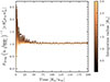 |
Fig. A.1. Time evolution of the gravitational drag measured within different logarithmically spaced integration radii, scaled by the Coulomb logarithm. We find the gravitational drag to follow the Coulomb-logarithm scaling in a quasi-steady state, provided bmin ≃ 0.78. |
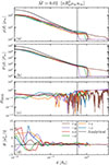 |
Fig. A.2. Same as Fig. 2 but for accretion parameters δ = 0 and γ = 100, corresponding to a mass accretion Ṁ ≃ 0.02 ṀHL in a quasi-steady state. |
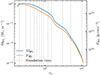 |
Fig. A.3. Hoyle–Lyttleton accretion rate and drag force as a function of the stratification parameter (ϵρ) for the 2 M⊙ red giant MESA model (see Fig. 1). Vertical dashed lines indicate the ϵρ values employed in the stratified simulations of this work. |
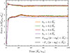 |
Fig. A.4. Time evolution of the radial and drag forces exerted by the gas on the companion in stratified simulations with ϵρ = 3, with different softening radii (hs). Forces are integrated within a sphere of radius |

 |
Fig. A.5. Inspiral of a 0.2 M⊙ companion through the envelope of a 2 M⊙ red giant, using four drag force prescriptions: our fitted drag and lift prescriptions (Eqs. 36–36b; solid blue); the prescription from De et al. (2020, orange); the Hoyle–Lyttleton formula, Fdrag = πRa2ρ∞u∞2 (green); and our fitted drag prescription but with F⊥ set to zero (dashed blue). For clarity, trajectories are shown only for r ≥ 0.25. Below this radius, trajectories start intersecting with themselves, corresponding to interaction with the companion’s own wake, which is not included in our model. At such small orbital separations, interactions with the primary’s wake would also play a major role in the orbital evolution. |
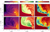 |
Fig. A.6. Zoomed-in snapshots in the xy plane of the density, pseudo-entropy, and Mach number at |


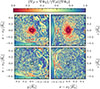 |
Fig. A.8. Close-up view of the normalized deviation from hydrostatic equilibrium in xy (left column) and xz (right column) planes at |


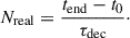
Appendix B: Simulation stochasticity
We performed 15 separate simulations, each initialized with a random perturbation δϵρ ∈ 0.5 × [ − 10−3, 10−3] to the background stratification parameter ϵρ = 0.5, in order to capture the system’s intrinsic stochastic behavior. This ensemble allows us to assess how much of the observed variability arises from inherent randomness, as opposed to variations in global parameters or added physical mechanisms such as magnetic fields, rotation, or accretion.
To quantify this stochasticity, we computed the autocorrelation function of the detrended drag force in each simulation run. We began with the raw drag force,  , and subtracted its best-fit linear trend to suppress spurious long-term correlations. To further reduce edge effects in the autocorrelation calculation, we mirrored the detrended signal by appending its time-reversed copy, following the method of Andrassy et al. (2022). The resulting time series,
  , was then used to compute the autocorrelation function over the interval
 ![Mathematical equation: $ t \in [t_0,\,t_{\mathrm{end}}]\,\widetilde{R_a}/u_{\infty} $](/articles/aa/full_html/2026/03/aa58057-25/aa58057-25-eq82.gif) :
:
 (B.1)
(B.1)
where t0 = 50 and tend = 100. The de-correlation time τdec is defined as the lag τ at which the normalized autocorrelation function R*(τ) first crosses zero. This provides a characteristic timescale over which fluctuations in the time series become approximately independent. For each realization, we estimated the number of independent fluctuations as
 (B.2)
(B.2)
For each realization, we computed the standard deviation σ0 of the original (not detrended) drag force Fdrag and estimate the standard error as
 (B.3)
(B.3)
Figure B.1 shows the time evolution of the drag force for all 15 simulations, including their individual time-averaged values over the interval ![Mathematical equation: $ t \in [t_0,\,t_{\mathrm{end}}], \widetilde{R_a}/u_{\infty} $](/articles/aa/full_html/2026/03/aa58057-25/aa58057-25-eq86.gif) , the standard error averaged across the realizations, and the autocorrelation function R(τ). We find that, for a softening radius
, the standard error averaged across the realizations, and the autocorrelation function R(τ). We find that, for a softening radius  , a stratification parameter ϵρ = 0.5 = δϵρ, and in the absence of accretion, the drag force exhibits significant time variability within each realization. However, the time-averaged drag forces differ by at most ∼4% across the 15 runs, with a 3σ range corresponding to a maximum relative variation of ∼17%. This range quantifies the baseline stochastic variability arising from small random perturbations in the stratification. The 3σ range observed here provides an illustration of the typical amplitude of fluctuations due to intrinsic stochasticity; their behavior under other physical conditions remains uncertain, however.
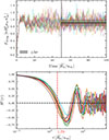 |
Fig. B.1. Top: Time evolution of the drag force exerted by the gas on the companion in 15 stratified simulations with ϵρ = 0.5 + δϵρ. Forces are integrated within a sphere of radius |

All Tables
All Figures
|
Fig. 1. Density and pressure profiles from the 2 M⊙ red giant MESA model of Ohlmann et al. (2016), shown as a function of the radius. Dashed lines indicate the polytropic reconstruction used as initial conditions, computed around the location where ϵρ = 3, which is marked by red crosses. The vertical line marks the radius where ϵρ = 10 in the reconstructed stellar structure. The red curve shows the stratification parameter (ϵρ) as a function of radius for the MESA model, while black dots indicate the ϵρ values employed in our simulations. |
| In the text | |
|
Fig. 2. Density (panel a), pressure (panel b), normalized hydrostatic balance residual RHSE = ∥∇P+ρ ∇Φ2∥/max(∥∇P∥, ∥ρ ∇Φ2∥) (panel c), and Bernoulli parameter (panel d) profiles along radial rays from the companion for a nonrotating, non-stratified, and non-accreting simulation with ℳ∞ = 4. Gray lines indicate the analytical solutions for density and pressure (Eqs. 25, 26) and the hydrostatic Bernoulli parameter ℬHSE (Eq. 31). The vertical dashed line marks the predicted shock radius, ds (Eq. 27). All quantities are averaged over a duration of Δt = Ra/u∞ once a quasi-steady state has been reached. |
| In the text | |
|
Fig. 3. Zoomed-in snapshots in the xy plane of the density, pseudo-entropy, and Mach number at t = 100 Ra/u∞ for non-stratified simulations with hs = 0.05 Ra and ℳ∞ = 4. First row: Non-accreting case. Second row: Accreting case with γ = 100 and δ = 0. |
| In the text | |
|
Fig. 4. Time evolution of the radial and drag forces exerted by the gas on the companion in non-stratified simulations with Ro = 5.5 and ℳ∞ = 4, with and without accretion. Forces are integrated within a sphere of radius 3 Ra. The shaded regions indicate the 3σ range (see Appendix B). |
| In the text | |
|
Fig. 5. Zoomed-in density, pseudo-entropy, and Mach number snapshots at t = 100 Ra/u∞ in the xy plane for non-stratified simulations with Ro = 5.5 and ℳ∞ = 2. The top panel includes rotation; the bottom does not. White lines indicate streamlines. |
| In the text | |
|
Fig. 6. Time evolution of the radial and drag forces exerted by the gas on the companion in non-stratified simulations with Ro = 5.5 and ℳ∞ = 2, with and without rotation. Forces are integrated within a sphere of radius 3Ra. The shaded regions indicate the 3σ range (see Appendix B). |
| In the text | |
|
Fig. 7. Zoomed-in snapshots of the density at |
| In the text | |
|
Fig. 8. Time-averaged drag (top) and lift (bottom) forces on the companion as functions of the stratification parameter (ϵρ) and integration radius, averaged over |
| In the text | |
|
Fig. 9. Normalized hydrostatic-centrifugal balance residual |
| In the text | |
|
Fig. A.1. Time evolution of the gravitational drag measured within different logarithmically spaced integration radii, scaled by the Coulomb logarithm. We find the gravitational drag to follow the Coulomb-logarithm scaling in a quasi-steady state, provided bmin ≃ 0.78. |
| In the text | |
|
Fig. A.2. Same as Fig. 2 but for accretion parameters δ = 0 and γ = 100, corresponding to a mass accretion Ṁ ≃ 0.02 ṀHL in a quasi-steady state. |
| In the text | |
|
Fig. A.3. Hoyle–Lyttleton accretion rate and drag force as a function of the stratification parameter (ϵρ) for the 2 M⊙ red giant MESA model (see Fig. 1). Vertical dashed lines indicate the ϵρ values employed in the stratified simulations of this work. |
| In the text | |
|
Fig. A.4. Time evolution of the radial and drag forces exerted by the gas on the companion in stratified simulations with ϵρ = 3, with different softening radii (hs). Forces are integrated within a sphere of radius |
| In the text | |
|
Fig. A.5. Inspiral of a 0.2 M⊙ companion through the envelope of a 2 M⊙ red giant, using four drag force prescriptions: our fitted drag and lift prescriptions (Eqs. 36–36b; solid blue); the prescription from De et al. (2020, orange); the Hoyle–Lyttleton formula, Fdrag = πRa2ρ∞u∞2 (green); and our fitted drag prescription but with F⊥ set to zero (dashed blue). For clarity, trajectories are shown only for r ≥ 0.25. Below this radius, trajectories start intersecting with themselves, corresponding to interaction with the companion’s own wake, which is not included in our model. At such small orbital separations, interactions with the primary’s wake would also play a major role in the orbital evolution. |
| In the text | |
|
Fig. A.6. Zoomed-in snapshots in the xy plane of the density, pseudo-entropy, and Mach number at |
| In the text | |
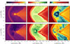 |
Fig. A.7. Same as Fig. A.6 but on a spherical shell at radius r2. |
| In the text | |
|
Fig. A.8. Close-up view of the normalized deviation from hydrostatic equilibrium in xy (left column) and xz (right column) planes at |
| In the text | |
|
Fig. B.1. Top: Time evolution of the drag force exerted by the gas on the companion in 15 stratified simulations with ϵρ = 0.5 + δϵρ. Forces are integrated within a sphere of radius |
| In the text | |
Current usage metrics show cumulative count of Article Views (full-text article views including HTML views, PDF and ePub downloads, according to the available data) and Abstracts Views on Vision4Press platform.
Data correspond to usage on the plateform after 2015. The current usage metrics is available 48-96 hours after online publication and is updated daily on week days.
Initial download of the metrics may take a while.