| Issue |
A&A
Volume 707, March 2026
|
|
|---|---|---|
| Article Number | A135 | |
| Number of page(s) | 8 | |
| Section | Planets, planetary systems, and small bodies | |
| DOI | https://doi.org/10.1051/0004-6361/202558167 | |
| Published online | 11 March 2026 | |
Exploring rotational properties and the YORP effect in asteroid families
1
Department of Physics and Astronomy, University of Padova,
Padova,
Italy
2
JSPS International Research Fellow, Department of Earth and Planetary Science, University of Tokyo,
Tokyo,
Japan
3
Université Côte d’Azur, Observatoire de la Côte d’Azur, CNRS, Laboratoire Lagrange,
Bd de l’Observatoire, CS 34229,
06304
Nice Cedex 4,
France
★ Corresponding authors: This email address is being protected from spambots. You need JavaScript enabled to view it.
; This email address is being protected from spambots. You need JavaScript enabled to view it.
Received:
18
November
2025
Accepted:
26
January
2026
Abstract
Context. The long-term dynamical evolution of asteroid families is governed by the interplay between orbital and rotational evolution driven by thermal forces and collision.
Aims. We aim to observationally trace the rotational evolution of main-belt asteroid families over gigayear timescales.
Methods. We analyzed rotational properties of 8739 asteroids with spin period measurements and 3794 asteroids with obliquity determinations across 28 asteroid families spanning ages from 14 Myr to 3 Gyr. We introduced a dimensionless timescale that normalizes each asteroid’s family age by its classical YORP timescale, enabling a direct comparison of the rotational states across different evolutionary stages. We examined two key observables: the fraction of slow rotators (periods greater than or equal to 30 hours) and the polarization fraction (the degree to which asteroid spin poles align correctly with their position in the family’s V-shape distribution according to the Yarkovsky theory). Evolution of both quantities were fit to identify characteristic transition timescales.
Results. We discovered that the slow-rotator fraction increases steeply with t and saturates at fslow ≃ 0.25 around a break point of tbp ≃ 20. This implies a stochastic YORP timescale of τYORP,stoc ≃ 10 τYORP in comparison with the rotational evolution models that include tumbling and weakened YORP torques. The polarization fraction reaches a maximum of ≃0.8 at t ≃ 16 and then decays toward the random limit fpol → 0.5 for t ≳ 20, indicating an increasing dominance of collisional spin reorientation over time.
Conclusions. The rotation properties within different asteroid families offer crucial clues to rotation evolution and can serve as a new dimension for the age estimation of asteroid families, particularly as more data will become available in the era of the Vera C. Rubin Observatory’s Legacy Survey of Space and Time (LSST).
Key words: methods: data analysis / catalogs / minor planets, asteroids: general
© The Authors 2026
 Open Access article, published by EDP Sciences, under the terms of the Creative Commons Attribution License (https://creativecommons.org/licenses/by/4.0), which permits unrestricted use, distribution, and reproduction in any medium, provided the original work is properly cited.
This article is published in open access under the Subscribe to Open model. This email address is being protected from spambots. You need JavaScript enabled to view it. to support open access publication.
1 Introduction
The modern asteroid belt is primarily composed of collisional fragments of planetesimals. Groups of fragments that share a common parent body are known as asteroid families (Hirayama 1918). The long-term dynamical evolution of asteroid families in the Solar System is significantly influenced by non-gravitational forces, such as the Yarkovsky effect, which arises from the anisotropic emission of thermal photons from the surface of a rotating body and results in an acceleration that secularly modifies the body’s semi-major axis.
The Yarkovsky-induced orbital drift of asteroids in the main belt is ~ 10−5−10−4 au Myr−1 for 1 km objects and scales as D−1, with D being the asteroid diameter (Bottke Jr et al. 2006; Spoto et al. 2015), and it leads to the orbital dispersion of the asteroid family. The predictable nature of the Yarkovsky effect has made it an invaluable tool for estimating the ages of asteroid families. Over time, this size-dependent dispersion creates a characteristic V-shape in a plot of a family’s semi-major axis versus the inverse diameter of its members. The analysis of this V-shape, combined with an independent evaluation of the Yarkovsky drift rate, enables estimation of the time elapsed since the formation of the family (e.g., Vokrouhlickỳ et al. 2006; Walsh et al. 2013; Milani et al. 2014; Delbo’ et al. 2017).
However, the evolution is complicated by the dependence of the Yarkovsky effect on several parameters that are difficult to determine, including thermal inertia and bulk density. Assuming a similar composition and surface properties across a given family, the remaining dependencies are spin rate and obliquity. The rotation of asteroids is mainly affected by collisions and a thermal torque known as YORP (Yarkovsky–O’Keefe–Radzievskii– Paddack) that is induced by the scattering and reemission of solar radiation from an asteroid’s irregular surface (Paddack 1969; Rubincam 2000). The YORP effect applies a torque that, over long timescales, can significantly modify its spin vector, altering both the spin period and the spin-axis obliquity. Collisions dominate large and slowly rotating asteroids, whereas YORP is more effective for small and fast rotators (Pravec et al. 2008).
In recent years, data from the Gaia mission (Gaia Collaboration 2023) have led to the computation ofa vast number of new asteroid spin vectors (Durech & Hanus 2023; Cellino et al. 2024). This wealth of data has revealed new and unexpected trends. For example, Durech & Hanus (2023); Cellino et al. (2024); Vavilov & Carry (2025) analyzed the spin period distribution and confirmed an excess of slow rotators that are separated by a “valley” from the population of fast rotators in the period-diameter diagram. This excess of slow rotators is explained by Zhou et al. (2025) as being the result of the gathering of the slowly tumbling asteroids (i.e., asteroids in non-principal axis rotation) that suffer from a weaker YORP torque.
The aim of this work is to investigate the rotational evolution of asteroids among asteroid families from the perspective of observation. We introduce a new parameterization built on general features of the Yarkovsky drift that are common to different families. As described in Sect. 2, by exploiting the estimated family ages, we introduce a normalized timescale that allows us to build a common framework of interpretation. In Sect. 3, we discuss our results, which show that the current dataset of rotational properties for the members of 28 families provides useful new constraints on the evolution timescales of the asteroid rotations. In Sect. 4 we summarize our findings.
2 Methods
We selected 28 asteroid families with ages ranging from 14.34 Myr (Nele) to 3024.13 Myr (Themis) (Spoto et al. 2015). The families and their properties are listed in Table A.1. The membership of each asteroid to a family and the proper elements were retrieved from the Asteroids Dynamic Site (Milani et al. 2014). We are aware that the estimation of family ages could be affected by methodological limitations and uncertainties in the Yarkovsky calibration. These problems are addressed in Sect. 2.3, which also contains an assessment of the impact of errors, when estimating the diameter, on the final result.
The diameter, D, and albedo, pV, were extracted from the WISE/NEOWISE survey (Masiero et al. 2011). For objects observed multiple times by the survey, we took the weighted average of their measurements using as weights the errors on D and pV. Since the absolute magnitude, H, does not have an error associated with the measure, we just calculated the mean.
To increase the statistics for objects that do not have a measurement for the diameter, we calculated D using
![Mathematical equation: $D = {{1329} \over {\sqrt {{{\hat p}_V}} }} \cdot {10^{ - 0.2H}}[{\rm{km}}],$](/articles/aa/full_html/2026/03/aa58167-25/aa58167-25-eq1.png) (1)
where
(1)
where  is the weighted average albedo of the family. Before the calculation of
  , possible outliers were discarded using the interquantile range. The absolute magnitude, H, was retrieved from the Asteroid Family Portal (Novaković et al. 2022). To calculate the error associated with
  , we performed a Monte Carlo bootstrap sampling of the errors associated with pV and took the median of this set. We repeated the operation 5000 times. In the end, we calculated the standard deviation of the set of the medians calculated above.
Spin vectors were retrieved from Cellino et al. (2024) and Durech & Hanus (2023). In addition, we also included data from the Asteroid Lightcurve Database (LCDB). From this last source, we selected only observations with a quality flag of Q ≥ 3−. For objects with more than one suitable measurement, we selected the most recent one (Warner et al. 2009). In the end, we obtained 8739 objects with a spin period and 3794 objects with obliquity estimation. The complete dataset is reported in the Zenodo repository1.
The lower statistics regarding the obliquity can be attributed to the difficulty in reconstructing light curves. The perioddiameter distribution of our sample is presented in Fig. 1, which further shows that this “valley” feature is present not only in the general asteroid population but also within individual families. It is important to note that the dataset is affected by observational biases. For example, it is easier to determine the spin state of fast rotators with respect to slow rotators because the latter require a longer observation time to cover a full rotation. Detecting super-fast rotators (P < 2.2 h) can also be challenging, particularly in sky surveys, due to an insufficient observation cadence (Novaković & Gutiérrez 2025). However, in our dataset only two asteroids, namely 1999 RF226 and 2008 VN1, can be classified as a super-fast rotator. In addition, the dataset is biased toward brighter asteroids, which are easier to observe.
We defined a dimensionless time, t, for each asteroid:
 (2)
where τage is the age of the family. Spoto et al. (2015) estimated the ages for both sides of the V-shape because families can be non-symmetrical in the (a, 1/D) space (e.g., in young families due to differences in the ejection velocities or in old families due to different impacts). For simplicity, we adopted the weighted average of the two age estimations, using as weights the errors associated with the measurements. The differences were taken into account in the error bars and are be addressed in Sect. 2.3.
(2)
where τage is the age of the family. Spoto et al. (2015) estimated the ages for both sides of the V-shape because families can be non-symmetrical in the (a, 1/D) space (e.g., in young families due to differences in the ejection velocities or in old families due to different impacts). For simplicity, we adopted the weighted average of the two age estimations, using as weights the errors associated with the measurements. The differences were taken into account in the error bars and are be addressed in Sect. 2.3.
The normal YORP timescale, τYORP, can be expressed as follows (Rubincam 2000; Vokrouhlickỳ & Čapek 2002; Golubov & Scheeres 2019):
![Mathematical equation: ${\tau _{{\rm{YORP}}}} \sim 1{\left( {{D \over {1\,{\rm{km}}}}} \right)^2}{\left( {{{{a_p}} \over {2.5{\rm{AU}}}}} \right)^2}\quad [{\rm{Myr}}].$](/articles/aa/full_html/2026/03/aa58167-25/aa58167-25-eq6.png) (3)
(3)
Here, D is the diameter of the asteroid, and ap is the proper semi-major axis. The YORP timescale is defined as the time it would take for an asteroid to double its rotation rate under the YORP torque (Rubincam 2000). The distribution of calculated r is shown in Fig. 2
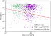 |
Fig. 1 Observational data from Gaia (in gray) showing the perioddiameter distribution for asteroids. As purple squares we show the distribution of the Hygeia family, and as green triangles we show the distribution of the Massalia family. The dashed red line is the fit line that identifies the gap (Zhou et al. 2025). Spin period values were calculated by Durech & Hanus (2023) and Cellino et al. (2024). The ages in the legend are the weighted average ages computed from Spoto et al. (2015). |
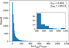 |
Fig. 2 Distribution of calculated t values for 8739 asteroids. The minimum t is tmin ≃ 0.003, while the maximum is tmax ≃ 1182.8. |
2.1 Fraction of slow rotators
The excess of slow rotators was discovered in the past century (e.g., Harris & Burns 1979; Pravec & Harris 2000; Durech & Hanus 2023). Zhou et al. (2025) shows that they could be in a tumbling state caused by YORP de-spin. As a result, this excess of slow rotators is expected to emerge on ~ 2 YORP timescales. To examine this condition, we investigated the fraction of slow rotators and its evolution among asteroid families, as their ages are known, and we assumed that the initial spin state was set immediately after the family forming event.
We binned the data with respect to t. For each time bin, ti, we calculated the fraction of slow rotators (i.e., asteroids with a rotation period P ≥ 30 hours):
 (4)
(4)
The error associated with the fraction is the 95% confidence interval of a binomial distribution. The error model used to compute the uncertainties on the bins is described in Appendix B. Based on a visual inspection of the data, it was clear that there is an increasing trend up to a certain value of t – a “break point.” After this point, the fraction of slow rotators remains roughly constant. For the analysis, we fixed the number of bins at 20: ten bins before and ten bins after the break point. This is a good compromise between the number of bins and the number of objects in each bin. The detailed fitting procedure is explained in Appendix B. The result for the best break point is  . The final fit of the data was done using an exponential-linear function described as
 (5)
(5)
The parameters for the best-fit result are presented in Table B.1. Figure 3 shows the fit function with the original asteroid data and synthetic data from Zhou et al. (2025) for comparison. The general trend of fslow increases and asymptotically converges to ~0.25, a result that we discuss in more detail in Sect. 3.
We note that the distribution of data points in t is not uniform. In particular, Fig. 2 shows an exponential decay of objects in the interval t ~ 200–450, which results in a visible gap in the binned trends shown in Fig. 3. This feature arises in the first place from the fact that we used a quantile function to bin the data (see Appendix B) and in the second place from the combined effect of the discrete age distribution of asteroid families, the strong dependence of t on the asteroid diameter (t ∝ D−2), and the observational incompleteness for small objects (≲ 6 km), especially in older families.
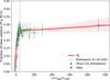 |
Fig. 3 Fraction of slow rotators as a function of the dimensionless time t. The green points are the binned-collected observational data in this work. Black triangles are simulation data from the Zhou et al. (2025) model, where the YORP timescale is manually increased by ten times compared to the normal YORP timescale. The red line is the fit function in Eq. (5). The shaded area is the 95% confidence interval of the fit. We do not show individual families because data are not sufficient for a statistical analysis. |
2.2 Polarization fraction
Another interesting feature to study is the distribution of spin poles inside a V-shape. It is known that the Yarkovsky effect also depends on the obliquity of the spin vector (Bottke Jr et al. 2006). The Yarkovsky effect is responsible for the V-shape distribution of an asteroid family in the (a − 1/D) space (Vokrouhlický et al. 2015). Prograde rotators drift outward in semi-major axis, while retrograde rotators drift inward. We therefore classified an asteroid as aligned when its spin sign, relative to the orbital plane, matches the position according to the expected drift direction. We also included spins with obliquities ε ~ 90°. We are aware that this may introduce some ambiguity due to the errors on the spin axis direction (several degrees) that may result in similar probabilities for both spin directions. However, this concerns a small number of cases, and they do not change the global statistics – the asteroids with 80° < ε < 100° correspond to 1.82% of the dataset.
The polarization fraction in each bin is then
 (6)
(6)
We again binned the data into ten bins before and ten bins after the break point.
The result for the best break point is  . The final values for the parameters were found fitting the following function to the data:
 (7)
(7)
The second half of the equation is an exponential decay function that approaches the value of 0.5, which is the expected value of the polarization fraction for a random distribution of spin vectors. The final result for the parameters is presented in Table B.1. The asteroid data and our fit are shown in Fig. 4, which shows that the function reaches the maximum value of ≃80% at t ≃ 15.07.
A similar gap in the t ~ 150–400 range is visible in the polarization fraction (Fig. 4) and has the same origin discussed in Sect. 2.1.
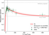 |
Fig. 4 Polarization fraction as a function of the dimensionless time t. The green points are the binned data; the red line is the fit function in Eq. (7). The black triangles are the distribution of the polarization fraction for the Eos family. The general trend is visible in single asteroid families. The shaded area is the 95% confidence interval of the fit. |
2.3 Assessing uncertainties
Each asteroid in the dataset is associated with uncertainties in its diameter, Di,err, and in the estimated age of its parent family, τage,err. Accounting for these sources of error may lead to variations in the inferred value of the optimal break point,  . In addition, the uncertainty on the family age reflects possible methodological limitations in the age determination and in the calibration of the Yarkovsky drift.
To assess the sensitivity of our results to these uncertainties, we performed a Monte Carlo resampling of the dataset. For each asteroid, we independently resampled the diameter and family age according to Di,ew ~ 𝒩(Di, Di,err) and τage,new ~ 𝒩(τage, τage,err), and we recomputed the corresponding dimensionless time, t. The resampled dataset was then analyzed using the same fitting procedure described in the previous sections and detailed in Appendix B, yielding anew estimate of the best break point. This procedure was repeated 500 times to build a distribution of break point values, from which we computed the median and the 95% confidence interval.
The resulting best estimations of the uncertainty-propagated break points are shown in Fig. 5, where they are compared with the original estimates. For the slow rotators fraction, we obtained  , while for the polarization fraction, we found
  .
.
To quantify the agreement between the original and uncertainty-propagated break point estimates, we employed a two-tailed probability-to-exceed (P.T.E.) test (Raveri & Hu 2019). We first computed the absolute difference between the median values,  , referred to as the “observed difference.” We then resampled with replacement both the original and the uncertainty-propagated break point distributions, and we computed the difference between their medians for each realization. The P.T.E. was finally obtained as the fraction of resampled differences exceeding the observed difference in absolute value.
The inclusion of uncertainties in diameter and family age produced only minor variations in the inferred break point locations. The uncertainty-propagated estimates show substantial overlap with the original determinations, with largely overlapping 95% confidence intervals and median values consistent within the corresponding uncertainty bands (Fig. 5). The resulting P.T.E. values are ≃48.4% for the slow-rotator fraction and ≃71.6% for the polarization fraction, indicating statistically compatible results and supporting the robustness of the original break point estimates.
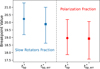 |
Fig. 5 Comparison between the best break point estimated from the original dataset, |


3 Implications
3.1 Excess of slow rotators
Our studies confirm the excess of slow rotators for the overall asteroid population. Significantly, for the first time, we have captured the process of its occurrence. We observed a rapid evolution in the fraction of slow rotators before the transition (t < 20.5), after which it converged to ~25%. This fraction is consistent with a previous study by Pravec et al. (2008). In their work, fslow ~ 20% was derived from 268 asteroids with diameters D=3–15 km. Of them, 79 are members of either the Hungaria or Phocaea family, and most of them are older than 4 Gyr.
In early studies, this excess was empirically modeled by artificially reducing spin acceleration by a factor of two Pravec et al. (2008) or by stopping rotational evolution Bottke et al. (2015) beyond a prescribed period. However, these approaches are not grounded in a self-consistent physical mechanism.
In the model of Zhou et al. (2025), tumbling was introduced for the first time, and the YORP torque acting on tumblers was reduced by a factor of ηtumbling = 10 due to isotropic radiation under a chaotic tumbling rotation. The free parameter ηtumbling was calibrated to reproduce the slow-rotator fraction measured by Pravec et al. (2008). Consequently, the tumblers spin up or down more slowly than spinners (i.e., those in principle-rotation), leading to an accumulation of asteroids in slow tumbling states and naturally producing an excess of slow rotators. Therefore, fslow is directly tied to the fraction of tumblers and increases with both η and the probability of a negative YORP torque. Figure 3 illustrates the evolution of fslow in the model of Zhou et al. (2025) for ηtumbling = 50.
3.2 The stochastic YORP timescale
We find that at t ~ 20.23, fslow starts to converge. In the models of Pravec et al. (2008) and Zhou et al. (2025), this corresponds to approximately two effective YORP timescales. The “static” YORP timescale, τYORP (Eq. (3)), refers to the time required for a body to evolve from its initial spin state to an end state under a fixed, unchanging YORP torque. In reality, however, YORP torques, and thus the evolution of the spin vector of an asteroid, often undergo a random walk (Bottke et al. 2015) because YORP is highly sensitive to small-scale surface features, such as craters and boulders, that may evolve (Statler 2009; Golubov & Krugly 2012; Cotto-Figueroa et al. 2015; Golubov & Lipatova 2022; Zhou et al. 2022; Zhou & Michel 2024).
To account for these stochastic processes, the effective YORP timescale is better represented by the “stochastic YORP timescale” rather than the “static” YORP timescale (Bottke et al. 2015), which can be estimated by
 (8)
where ηstoc describes the random-walk evolution of the YORP torque over the body’s collisional history. This modifies not only the rotation evolution rate but also the Yarkovsky-driven spreading and V-shape evolution of asteroid families. However, ηstoc remains largely uncertain due to the complexity of the models.
(8)
where ηstoc describes the random-walk evolution of the YORP torque over the body’s collisional history. This modifies not only the rotation evolution rate but also the Yarkovsky-driven spreading and V-shape evolution of asteroid families. However, ηstoc remains largely uncertain due to the complexity of the models.
This study provides the first direct observational validation of these theoretical predictions through our examination of the rotational evolution of asteroid families spanning a broad range of ages. The rotational model predicts that fslow converges at ~2τYORP,stoc (Pravec et al. 2008; Zhou et al. 2025). Figure 3 shows both the observational asteroid data collected in this study and the simulation data from the model of Zhou et al. (2025), where the YORP timescale was manually increased by a factor of ten. The agreement between the simulation data and observations supports the stochastic YORP timescale being roughly an order of magnitude longer than the classical YORP timescale (i.e., ηstoc 10).
Given such a long stochastic YORP timescale, in combination with the interplay of collisions, YORP self-limitation could be triggered. Significantly, this phenomenon could explain why small asteroids evade transformation into top shapes and/or binaries. This is achieved by their rotational rates being constrained, thereby regulating the amount of angular momentum that can be imparted to a deformable body (Cotto-Figueroa et al. 2015). With YORP evolution proceeding about 20 times slower than classically predicted, many asteroids simply do not experience sufficient YORP cycles within their dynamical lifetimes to undergo catastrophic reshaping.
3.3 Polarization fraction
The evolution of the polarization fraction provides insight into the interplay between YORP-driven spin evolution and collisional reorientation. At early evolutionary stages (t ≲ 18.96), the polarization fraction increases, reaching a maximum of ≃80% at t ≃ 15.07. This rise indicates that Yarkovsky initially dominates the orbital evolution in the semi-major axis space, systematically aligning the asteroid spin axes with their orbital drift direction. In this initial stage, the YORP effect could increase the efficiency of the Yarkovsky drift by driving asteroids toward extreme obliquities (0° or 180°), thereby enhancing the correlation between spin orientation and semi-major axis position within the V-shape. However, the fact that polarization reaches only 80% rather than complete alignment suggests a combination of stochastic reorientation due to collisions and errors in the currently determined spin directions, the precise proportions of which remain unknown.
The subsequent decay of polarization to 0.5 at a larger t indicates complete randomization of spin axes relative to the orbital position. This transition suggests that collisional reorientation becomes increasingly important relative to Yarkovsky- and YORP-driven evolution at extended timescales. The cumulative effect of non-catastrophic collisions progressively breaks the connection between the current spin state and the Yarkovsky drift history that determined the asteroid’s position in the V-shape. This interpretation is consistent with theoretical models suggesting that for smaller objects (i.e., more evolved family members), collisions occur more frequently and with greater strength, causing bodies to transition between different spin states more rapidly (Marzari et al. 2011).
The randomization of spin axes through collisions has implications for the interpretation of asteroid family ages derived from the V-shape. The fundamental hypothesis underlying V-shape age dating is that the direction and drift rate of the semi-major axis for family members located at the edges of the V-shape remain constant over time (Milani et al. 2014). However, collisional spin reorientation introduces a random-walk component to the Yarkovsky drift. Under these conditions, the inverse slopes of the V-shape borders are no longer proportional to the family age. Instead, they scale with the square root of the family age (Marzari et al. 2011). The decay of polarization toward a random state at large dimensionless times indicates that collisional spin reorientation becomes increasingly important for family members older than t ≈ 20, marking the limit beyond which V-shape age estimates become unreliable. For older families, partial erasure of the Yarkovsky signature may bias V-shape results. In such cases, the degree of polarization could serve as an independent diagnostic or correction factor. Further work is needed to quantify these effects.
4 Conclusions
In this work, we have utilized the rapidly expanding dataset of asteroid spin states to empirically investigate the long-term rotational evolution of main-belt asteroid families. By introducing a dimensionless evolutionary timescale (t = τage/τYORP), we directly compared 28 asteroid families with a wide range of ages and provided new observational constraints on the coupled YORP-Yarkovsky collision processes.
We showed that the fraction of slow rotators increases rapidly with t and saturates at 0.25 near t ≈ 20. This behavior matches theoretical predictions for the onset of stochastic YORP selflimitation and yields an effective stochastic YORP timescale ten times longer than the classical formulation (ηstoc 10). Our results therefore provide the first direct population-level confirmation that YORP evolution is significantly slowed by surface-morphology-driven torque variability.
We further showed that the polarization fraction – quantifying the spin–orbit correlation within V-shapes – initially rises to ~80% as YORP drives bodies toward extreme obliquities and efficient Yarkovsky drift. However, beyond t ≈ 20, the polarization decays toward the random limit of ~50%, indicating that collisional reorientation increasingly dominates the spin evolution of older families. This transition marks the approximate age boundary beyond which V-shape estimates become systematically biased and suggests that the degree of polarization may be used as a diagnostic or correction factor for advanced families.
The rotational evolution trends of fslow and fpol can be further tested with the forthcoming Vera C. Rubin Observatory’s Legacy Survey of Space and Time (LSST), which is expected to increase the available spin-state sample by at least an order of magnitude (Ivezić et al. 2019). With such datasets, these trends could provide an additional dimension for constraining asteroid family ages, for example, by fitting τage to the evolutionary tracks in Figs. 3 and 4 for individual families.
Acknowledgements
W.-H. Zhou acknowledges funding support from the Japan Society for the Promotion of Science (No. P25021). G. Bertinelli thanks G. Viterbo for helpful discussions on topics related to this work. The authors thank the anonymous referee for productive comments and suggestions.
References
- Bottke, W. F., Vokrouhlický, D., Walsh, K. J., et al. 2015, Icarus, 247, 191 [CrossRef] [Google Scholar]
- Bottke Jr, W. F., Vokrouhlický, D., Rubincam, D. P., & Nesvorný, D. 2006, Annu. Rev. Earth Planet. Sci., 34, 157 [CrossRef] [Google Scholar]
- Burnham, K. P., & Anderson, D. R., eds. 2004, Model Selection and Multimodel Inference (Springer New York) [Google Scholar]
- Cellino, A., Tanga, P., Muinonen, K., & Mignard, F. 2024, A&A, 687, A277 [NASA ADS] [CrossRef] [EDP Sciences] [Google Scholar]
- Cotto-Figueroa, D., Statler, T. S., Richardson, D. C., & Tanga, P. 2015, ApJ, 803, 25 [NASA ADS] [CrossRef] [Google Scholar]
- Delbo’, M., Walsh, K., Bolin, B., Avdellidou, C., & Morbidelli, A. 2017, Science, 357, 1026 [NASA ADS] [CrossRef] [Google Scholar]
- Durech, J., & Hanus, J. 2023, A&A, 675, A24 [NASA ADS] [CrossRef] [EDP Sciences] [Google Scholar]
- Gaia Collaboration (Galluccio, L., et al.) 2023, A&A, 674, A35 [NASA ADS] [CrossRef] [EDP Sciences] [Google Scholar]
- Golubov, O., & Krugly, Y. N. 2012, ApJ, 752, L11 [NASA ADS] [CrossRef] [Google Scholar]
- Golubov, O., & Lipatova, V. 2022, A&A, 666, A146 [NASA ADS] [CrossRef] [EDP Sciences] [Google Scholar]
- Golubov, O., & Scheeres, D. J. 2019, AJ, 157, 105 [NASA ADS] [CrossRef] [Google Scholar]
- Harris, A. W., & Burns, J. A. 1979, Icarus, 40, 115 [Google Scholar]
- Hirayama, K. 1918, AJ, 31, 185 [Google Scholar]
- Huber, P. J. 1964, Ann. Math. Statist., 35, 73 [Google Scholar]
- Ivezić, Ž., Kahn, S. M., Tyson, J. A., et al. 2019, ApJ, 873, 111 [Google Scholar]
- Marzari, F., Rossi, A., & Scheeres, D. 2011, Icarus, 214, 622 [NASA ADS] [CrossRef] [Google Scholar]
- Masiero, J. R., Mainzer, A. K., Grav, T., et al. 2011, ApJ, 741, 68 [Google Scholar]
- Milani, A., Cellino, A., Knežević, Z., et al. 2014, Icarus, 239, 46 [NASA ADS] [CrossRef] [Google Scholar]
- Newcombe, R. G. 1998, Statist. Med., 17, 857 [Google Scholar]
- Novaković, B., & Gutiérrez, P. J. 2025, AJ, 170, 248 [Google Scholar]
- Novaković, B., Vokrouhlický, D., Spoto, F., & Nesvorný, D. 2022, Celest. Mech. Dyn. Astron., 134, 34 [NASA ADS] [CrossRef] [Google Scholar]
- Paddack, S. J. 1969, J. Geophys. Res., 74, 4379 [NASA ADS] [CrossRef] [Google Scholar]
- Pravec, P., & Harris, A. W. 2000, Icarus, 148, 12 [NASA ADS] [CrossRef] [Google Scholar]
- Pravec, P., Harris, A. W., Vokrouhlický, D., et al. 2008, Icarus, 197, 497 [NASA ADS] [CrossRef] [Google Scholar]
- Raveri, M., & Hu, W. 2019, Phys. Rev. D, 99 [Google Scholar]
- Rubincam, D. P. 2000, Icarus, 148, 2 [Google Scholar]
- Spoto, F., Milani, A., & Knežević, Z. 2015, Icarus, 257, 275 [NASA ADS] [CrossRef] [Google Scholar]
- Statler, T. S. 2009, Icarus, 202, 502 [NASA ADS] [CrossRef] [Google Scholar]
- Vavilov, D., & Carry, B. 2025, A&A, 693, A66 [NASA ADS] [CrossRef] [EDP Sciences] [Google Scholar]
- Vokrouhlickỳ, D., & Čapek, D. 2002, Icarus, 159, 449 [CrossRef] [Google Scholar]
- Vokrouhlickỳ, D., Brož, M., Morbidelli, A., et al. 2006, Icarus, 182, 92 [CrossRef] [Google Scholar]
- Vokrouhlický, D., Bottke, W. F., Chesley, S. R., Scheeres, D. J., & Statler, T. S. 2015, in Asteroids IV, eds. P. Michel, F. E. DeMeo, & W. F. Bottke (University of Arizona Press) [Google Scholar]
- Walsh, K. J., Delbo, M., Bottke, W. F., Vokrouhlický, D., & Lauretta, D. S. 2013, Icarus, 225, 283 [NASA ADS] [CrossRef] [Google Scholar]
- Warner, B., Harris, A., & Pravec, P. 2009, Asteroid Lightcurve Database (LCDB), updated: 2023 October 1 [Google Scholar]
- Zhou, W.-H., & Michel, P. 2024, A&A, 682, A130 [NASA ADS] [CrossRef] [EDP Sciences] [Google Scholar]
- Zhou, W.-H., Zhang, Y., Yan, X., & Michel, P. 2022, A&A, 668, A70 [NASA ADS] [CrossRef] [EDP Sciences] [Google Scholar]
- Zhou, W.-H., Michel, P., Delbo, M., et al. 2025, Nat. Astron., 9, 493 [Google Scholar]
pandas.qcut
Appendix A Asteroid families
List of the 28 families used in the analysis.
Appendix B Fitting procedure
Since the distribution of t (Eq. 2) is not uniform (see Fig. 2), we used the quantile-based discretization function2 to roughly have the same number of asteroids in each bin. The value of t at which each bin is centered is associated with an error, given by the standard deviation of the dimensionless times inside the bin. The fraction of slow rotators in each bin is calculated as the number of slow rotators divided by the total number of asteroids in the bin. The error associated with the fraction is the 95% confidence interval of a binomial distribution. In particular, we used the Wilson score interval with continuity correction (Newcombe 1998).
We fit the data with respect to the slow rotators fraction (Sect. 2.1), with a piecewise function defined as
 (B.1)
where tbp is the break point and a, j, k, m, and b are the parameters to be fit.
(B.1)
where tbp is the break point and a, j, k, m, and b are the parameters to be fit.
Parameter estimation We employed a weighted Huber loss function to ensure robustness against outliers:
 (B.2)
where δ = 1.345 (Huber 1964). The weighted residual r accounts for error propagation through
(B.2)
where δ = 1.345 (Huber 1964). The weighted residual r accounts for error propagation through  , where yerr and terr are the errors associated with the fraction of slow rotators (polarization) and with t, respectively. Since the error on the fraction of slow rotators (polarization) is asymmetric (from the Wilson confidence interval), we adopted the following scheme:
 otherwise.
The total loss was calculated as ℒHuber = Σi L(ri). The Huber loss provides robust parameter estimates that are less sensitive to outliers compared to ordinary least squares, and does not require errors to be normally distributed (Huber 1964).
Break point selection We implemented an iterative scan over candidate tbp values to identify the optimal model complexity· At each candidate break point, we fit the model parameters using the Huber loss, then evaluated model quality using the Akaike information criterion (AIC):
 (B.3)
where k is the effective number of free parameters, n is the number of data points, and RSS is the weighted residual sum of squares:
(B.3)
where k is the effective number of free parameters, n is the number of data points, and RSS is the weighted residual sum of squares:
 (B.4)
(B.4)
Note that while parameter estimation used the Huber loss, model selection employed RSS for AIC calculation to maintain consistency with standard information-theoretic model comparison (Burnham & Anderson 2004)· The AIC penalizes model complexity and prevents overfitting, with lower values indicating better models· The break point that minimized AIC was selected as optimal·
The parameters were fit using the Sequential Least Squares Programming (SLSQP) algorithm from the SciPy package in Python, with an equality constraint enforcing the continuity of f(t) at tbp.
The scan was initialized with a wide range of tbp values and then refined by manually reducing, in an iterative fashion, the interval around the values that provided the lowest AIC value· To have a statistical estimate of the parameters, we performed a Monte Carlo bootstrap sampling of the data, i.e., we randomly sampled the data with replacement and fit the piecewise function to each set· We repeated the process 500 times· The values of the final parameters are the median of the distribution obtained from the procedure, while the errors are given by the 95% confidence interval of the distributions.
The fitting procedure for the polarization fraction (Sect. 2.2) is the same as explained above, and the best break point  was found by fitting the following function:
 (B.5)
(B.5)
The second part of the piecewise function is an exponential decay function that approaches the value of 0.5, which is the expected value of the polarization fraction for a random distribution of spin vectors.
In the end, for both the slow rotators fraction and the polarization fraction, we fit the data with a unique function (Eq. 5 and Eq. 7, respectively), fixing the break point at  . The final parameters were again obtained from a Monte Carlo bootstrap sampling after 1000 simulations.
All Tables
All Figures
|
Fig. 1 Observational data from Gaia (in gray) showing the perioddiameter distribution for asteroids. As purple squares we show the distribution of the Hygeia family, and as green triangles we show the distribution of the Massalia family. The dashed red line is the fit line that identifies the gap (Zhou et al. 2025). Spin period values were calculated by Durech & Hanus (2023) and Cellino et al. (2024). The ages in the legend are the weighted average ages computed from Spoto et al. (2015). |
| In the text | |
|
Fig. 2 Distribution of calculated t values for 8739 asteroids. The minimum t is tmin ≃ 0.003, while the maximum is tmax ≃ 1182.8. |
| In the text | |
|
Fig. 3 Fraction of slow rotators as a function of the dimensionless time t. The green points are the binned-collected observational data in this work. Black triangles are simulation data from the Zhou et al. (2025) model, where the YORP timescale is manually increased by ten times compared to the normal YORP timescale. The red line is the fit function in Eq. (5). The shaded area is the 95% confidence interval of the fit. We do not show individual families because data are not sufficient for a statistical analysis. |
| In the text | |
|
Fig. 4 Polarization fraction as a function of the dimensionless time t. The green points are the binned data; the red line is the fit function in Eq. (7). The black triangles are the distribution of the polarization fraction for the Eos family. The general trend is visible in single asteroid families. The shaded area is the 95% confidence interval of the fit. |
| In the text | |
|
Fig. 5 Comparison between the best break point estimated from the original dataset, |
| In the text | |
Current usage metrics show cumulative count of Article Views (full-text article views including HTML views, PDF and ePub downloads, according to the available data) and Abstracts Views on Vision4Press platform.
Data correspond to usage on the plateform after 2015. The current usage metrics is available 48-96 hours after online publication and is updated daily on week days.
Initial download of the metrics may take a while.