| Issue |
A&A
Volume 707, March 2026
|
|
|---|---|---|
| Article Number | A154 | |
| Number of page(s) | 14 | |
| Section | Extragalactic astronomy | |
| DOI | https://doi.org/10.1051/0004-6361/202558176 | |
| Published online | 03 March 2026 | |
IXPE and VLT/FORS2 polarimetry challenge the Seyfert-1.9 classification of MCG-05-23-16
1
Université de Strasbourg, CNRS, Observatoire Astronomique de Strasbourg, UMR 7550 11 rue de l’Université 67000 Strasbourg, France
2
Dipartimento di Matematica e Fisica, Università degli Studi Roma Tre via della Vasca Navale 84 00146 Roma, Italy
3
Institut d’Astrophysique et de Géophysique, Université de Liège, Allée du 6 Août 19c B5c 4000 Liège, Belgium
4
National Astronomical Observatory of Japan, National Institutes of Natural Sciences 2-21-1 Osawa Mitaka Tokyo 181-8588, Japan
5
NASA Marshall Space Flight Center Huntsville AL 35812, USA
6
Astronomical Institute of the Czech Academy of Sciences Boční II 1401/1 14100 Praha 4, Czech Republic
7
Department of Physics and Astronomy, Clemson University Kinard Lab of Physics Clemson SC 29634, USA
8
Department of Physics, Washington University St. Louis MO 63130, USA
9
McDonnell Center for the Space Sciences, Washington University St. Louis MO 63130, USA
10
Center for Quantum Leaps, Washington University St. Louis MO 63130, USA
11
ASI – Agenzia Spaziale Italiana Via del Politecnico snc 00133 Roma, Italy
12
MIT Kavli Institute for Astrophysics and Space Research, Massachusetts Institute of Technology 77 Massachusetts Avenue Cambridge MA 02139, USA
13
INAF Osservatorio Astronomico di Roma Via Frascati 33 00078 Monte Porzio Catone RM, Italy
14
Université Grenoble Alpes, CNRS, IPAG 38000 Grenoble, France
15
Space Science Data Center, Agenzia Spaziale Italiana Via del Politecnico snc 00133 Roma, Italy
16
Instituto de Estudios Astrofísicos, Facultad de Ingeniería y Ciencias, Universidad Diego Portales Avenida Ejército Libertador 441 Santiago, Chile
17
Dipartimento di Fisica, Universitá degli Studi di Roma “Tor Vergata”, Via della Ricerca Scientifica 1 00133 Roma, Italy
18
Istituto Nazionale di Fisica Nucleare, Sezione di Roma “Tor Vergata”, Via della Ricerca Scientifica 1 00133 Roma, Italy
★ Corresponding author: This email address is being protected from spambots. You need JavaScript enabled to view it.
Received:
19
November
2025
Accepted:
19
January
2026
Abstract
We report the third observation of the Seyfert-1.9 active galactic nucleus (AGN) MCG-05-23-16 with the Imaging X-ray Polarimetry Explorer (IXPE), together with optical spectropolarimetry obtained at the Very Large Telescope (VLT), and combined with archival near-ultraviolet, optical, and near-infrared polarimetric data. We detect no X-ray polarization in the 2–8 keV band, with a 99% confidence upper limit of ≤2.9%, which is further reduced to ≤2.5% when combined with the two previous IXPE observations of the same target. Monte Carlo simulations suggest that equatorial coronal models are disfavored if the AGN is indeed a type 1.9/2 AGN, while coronae coplanar to the accretion disk remain consistent if the source is less inclined than previously assumed. Data from VLT/FORS2 reveal a typical type 2 spectrum in total flux, a broad Hα line in polarized flux, and a polarization degree and angle that depend strongly on wavelength. The polarization angle rotates by nearly 70° across the optical band. Comparison with historical measurements confirms the long-term stability of the polarization spectrum and a ∼90° rotation in the near-ultraviolet. Interpreting the multiwavelength polarization relative to the AGN ionization axis indicates that the main obscurer is not a compact circumnuclear torus, but rather a distant kiloparsec-scale dust lane crossing the galaxy. This result implies that MCG-05-23-16 is, in fact, a type 1 AGN seen through foreground dust. The low X-ray column density becomes consistent with the absence of polarization, provided that the nuclear inclination is low.
Key words: polarization / galaxies: active / galaxies: individual: MCG-05-23-16 / galaxies: Seyfert / X-rays: general
© The Authors 2026
 Open Access article, published by EDP Sciences, under the terms of the Creative Commons Attribution License (https://creativecommons.org/licenses/by/4.0), which permits unrestricted use, distribution, and reproduction in any medium, provided the original work is properly cited.
This article is published in open access under the Subscribe to Open model. This email address is being protected from spambots. You need JavaScript enabled to view it. to support open access publication.
1. Introduction
X-ray polarimetry has proven to be a powerful tool for probing the energy generation mechanisms at the heart of spatially unresolved sources. High-energy polarimetric measurements obtained with the Imaging X-ray Polarimetry Explorer (IXPE; Weisskopf et al. 2022) demonstrate that the region responsible for X-ray emission (a hot electron plasma located near the accretion disk) is likely extended along the disk plane rather than being compact and aligned with the disk symmetry axis, as commonly assumed in the lamppost geometry (Miniutti & Fabian 2004). This result holds across a wide range of sources, from microquasars in the hard state (see, e.g., Krawczynski et al. 2022) to active galactic nuclei (AGNs) that are little or not obscured (Gianolli et al. 2023). Two arguments support this conclusion: a high degree of linear polarization (several percent) and a polarization angle parallel to the axis traced by the radio structure or jets, indicating that the polarization emerges from scattering in a nonspherical equatorial region. By contrast, a more symmetric geometry (e.g., spherical) would reduce the polarization degree, and any other location (for example, along the polar axis of the object) would lead to a different polarization angle (Ursini et al. 2022).
NGC 4151 was the first radio-quiet, pole-on object in which X-ray polarimetry demonstrated that the X-ray corona is likely extended along the equatorial plane (Gianolli et al. 2023, 2024). IC 4329A, another unobscured AGN, appears to corroborate these findings, but the results are less statistically significant (Ingram et al. 2023). However, X-ray polarimetric data obtained with IXPE remain inconclusive for NGC 2110 (Chakraborty et al. 2025) and for MCG-05-23-16. This latter AGN is particularly interesting because, despite two pointings (May and October 2022), totaling 1128 Ms – the largest exposure time for a radio-quiet, pole-on object – only an upper limit of 3.2% at 99% confidence level has been inferred (Marinucci et al. 2022; Tagliacozzo et al. 2023). The polarization angle remains unconstrained. This result is puzzling because MCG-05-23-16 is, among the unobscured AGNs observed by IXPE (NH ∼ 1022 cm−2, Mattson & Weaver 2004), the source with the greatest estimated inclination (from 33° to 65°, depending on the method; see Turner et al. 1998; Reeves et al. 2007; Fuller et al. 2016; Serafinelli et al. 2023), which should lead to high levels of X-ray polarization.
MCG-05-23-16 is a type 1.9 AGN, which means that its optical broad emission lines are not detected in total flux. Only broad infrared emission lines (such as Paβ emission) are detected, due to the decreasing impact of dust extinction in the infrared (Goodrich et al. 1994). Broad lines are present in the optical spectrum of MCG-05-23-16, but they appear only in polarized light, owing to scattering off the polar wind material (Lumsden et al. 2004). This indicates a large nuclear inclination and, consequently, a large scattering-induced polarization. Despite its brightness (F2−10 keV = 7–10 × 10−11 erg cm−2 s−1, Mattson & Weaver 2004), no X-ray polarization was detected from MCG-05-23-16. This either indicates that the source is much less inclined than previously estimated, or that its X-ray corona sustains an intrinsically lower polarization fraction, pointing to a geometrical and physical configuration different from all other unobscured AGNs and microquasars in the hard state observed by IXPE.
To address this issue, we conducted a third observation of MCG-05-23-16 with IXPE, combining the 2022 data with those obtained in 2025. We supplemented the latter with a new XMM-Newton observation to assess the spectral-shape stability and disentangle the polarization contributions from different spectral components.
2. X-ray observations and data reduction
The IXPE observed MCG-05-23-16 on two previous occasions: in May 2022 (Marinucci et al. 2022) and November 2022 (Tagliacozzo et al. 2023). The IXPE observation, performed simultaneously with XMM-Newton (for the first observation only) and NuSTAR (for both campaigns), had net exposure times of 486 ks and 642 ks, respectively. In this study, we used both datasets with updated response matrices. The third pointing, which constitutes the observation reported here, took place between April 24 and May 9, 2025. However, one of the three detector units (DUs) of IXPE – DU2 specifically – suffered from an anomaly, and we therefore excluded it from the present analysis. The remaining two DUs (DU1 and 3) combined a total exposure of 745 ks. We first processed the cleaned level 2 event files using the background rejection procedure described in Di Marco et al. (2023), then applied standard filtering criteria using the dedicated ftools tasks and the latest IXPE CALDB (20250225) calibration files. We followed the formalism described by Strohmayer (2017), applying the weighted analysis method detailed in Di Marco et al. (2022), with stokes=Neff set in xselect. We extracted the I, Q, and U Stokes background spectra from source-centered annular regions with an internal radius of 150 arcsec and an external radius of 300 arcsec. We optimized the source extraction regions to maximize the signal-to-noise ratio (S/N) in the 2–8 keV band, following the procedure described by Piconcelli et al. (2004), resulting in radii of 85 arcsec and 80 arcsec for the first and third DUs, respectively. We applied these same radii, centered on the source, to the I, Q, and U spectra. After processing, we obtained a net exposure time of 740 ks. We adopted a constant energy binning of 0.2 keV for the Q and U Stokes spectra, with a minimum S/N of three required in each bin of the intensity spectra. The background contribution during the 2025 observation amounted to 2.4% for each DU, comparable to the values of 2022.
XMM-Newton observed MCG-05-23-16 on May 8, 2025, with an elapsed time of 87.2 ks using the European Photon Imaging Camera (EPIC) charge-coupled device (CCD) cameras: the pn (Strüder et al. 2001) and the two Metal Oxide Semi-conductor (MOS) CCD arrays (Turner et al. 2001), operated in small window and medium filter mode. We excluded data from the MOS detectors from the analysis due to pile-up, while the pn camera data did not show a significant pile-up, as confirmed by the EPATPLOT output. We computed the extraction radii and optimal time cuts for background flares using SAS 22.1 (Gabriel et al. 2004), applying the same S/N maximization procedure as in previous observations. The resulting optimal extraction radii for the source and background spectra were 40 and 50 arcsec, respectively. The net exposure time for the pn time-averaged spectrum after filtering was 58.4 ks.
We present the background-subtracted light curves for all observations in the appendices.
3. Results and analysis
3.1. IXPE campaign
First, we performed a preliminary analysis of the IXPE data alone, using XSPEC v12.13.1e (Arnaud 1996) and a baseline model consisting of an absorbed power law convolved with a constant polarization kernel, as in Tagliacozzo et al. (2023): const × polconst × tbabs × ztbabs × powerlaw. We applied this model to the third IXPE observation of MCG-05-23-16 (April 2025; 740 ks), simultaneously fitting the I, Q, and U spectra from the two available DUs over the 2–8 keV energy range. When relying solely on IXPE data, more complex models are unnecessary, as evidenced by the reduced chi-square values, which are consistently close to one (χ2/d.o.f. = 415/405). The multiplicative constant accounts for cross-calibration uncertainties between DU1 and DU3. We modeled Galactic absorption along the line of sight with tbabs, assuming a column density of NH, Gal = 7.8 × 1020 cm−2 (HI4PI Collaboration 2016). Freezing the column density at the redshift of the source (z = 0.00849) to the value derived from a broadband data analysis (see Sect. 3.2: NH, z = 1.48 × 1022 cm−2), we obtain a primary continuum spectral index of Γ = 1.84 ± 0.01. The left panel of Fig. 1 presents the Q and U spectra used in this initial analysis (including the model and residuals), while the right panel shows the contour plot between the polarization degree P and the polarization angle θ for the third IXPE observation.
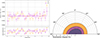 |
Fig. 1. Left panel: Stokes spectra Q (orange crosses) and U (magenta crosses) from the third IXPE pointing (April 2025) of MCG-05-23-16, shown with residuals and the corresponding best-fitting model. Right panel: Contour plot of the polarization degree P versus the polarization angle θ, summed over the 2 − 8 keV energy band of the third IXPE pointing. Purple, pink, and orange regions correspond to the 68%, 90%, and 99% confidence levels, respectively, for two parameters of interest. |
In contrast to the first and second observations of this source, the polarization degree is not constrained, even at the 68% confidence level. At the 99% confidence level, we find an upper limit of P = 3.0%. In addition, we do not find any significant variation in the polarization when evaluating smaller energy bins (i.e., we do not observe any polarization energy trend). Compared to the 2022 observations (for which we recomputed the numbers using the latest calibration files and the same baseline model), our 2025 campaign provides similar results (see Table 1). The polarization from the X-ray corona is consistent within 1σ across the three epochs.
X-ray polarimetry of MCG-05-23-16 using model-independent analyses.
Next, we performed a combined analysis of the IXPEI, Q, and U spectra collected in May and November 2022, and in April 2025, using the same model and leaving the spectral indices of the three pointings untied. As a result, we obtained the same value for the first two observations (Γ1 = Γ2 = 1.89 ± 0.01) and Γ3 = 1.81 ± 0.01 for the third. From this analysis, we obtain a polarization degree P = 1.0 ± 0.6% and a polarization angle θ = 53° ±18° at the 68% confidence level for one parameter of interest. This corresponds to an upper limit on the polarization degree upper of 2.5% at the 99% confidence level. This represents a significant improvement with respect to previously obtained results (see Table 1 for the best-fit values of the polarization degree and angle obtained using only the IXPE dataset). Fig. 2 shows the contour plots of the first observation, the first and the second combined, and for all three observations combined.
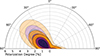 |
Fig. 2. Contour plots of the polarization degree P and angle θ for the May 2022 observation (dotted contours), May 2022 and November 2022 (dashed contours), and for the May 2022, November 2022, and April 2025 observations combined (solid contours). Contours colors are the same as in Fig. 1. |
3.2. Broadband spectral analysis
To obtain a comprehensive understanding of the system and derive parameters relevant for a useful spectropolarimetric analysis, we conducted a broadband X-ray spectral analysis by combining the full set of IXPEI Stokes parameter spectra (May and November 2022, and the 2025 campaign) with the 3–79 keV NuSTAR spectra (May and November 2022) and the 2–10 keV XMM-Newton spectra (May 2022 and April 2025).
Following the methodology of Serafinelli et al. (2023), we built the model const × tbabs × ztbabs [zcutoffpl + vashift(relxill + xillver)], where tbabs accounts for Galactic absorption (assuming a column density of NH, Gal = 7.8 × 1020 cm−2; HI4PI Collaboration 2016) and ztbabs accounts for column density at the source redshift. We also used zcutoffpl to model the primary continuum, while we used relxill and xillver for relativistic reflection from an ionized disk (emissivity profile ϵ(r)∝r−3) and distant neutral reflection (e.g., from the torus or the outer disk), respectively. These components share the same photon index and cutoff energy of the primary continuum. The constant multiplicative component accounts for cross-calibration uncertainties among the various instruments (IXPE DUs, NuSTAR FPMA and FPMB, and XMM-Newton EPIC-pn). As in previous studies (Marinucci et al. 2022; Tagliacozzo et al. 2023; Serafinelli et al. 2023), we included a vashift component, which provides an energy shift 6.4 keV in the host galaxy rest frame. This effect is observed in the 2022 XMM/pn (but not MOS) data and in the NuSTAR/FPMA and FPMB observations (with an increasing deviation between the first and the second pointings) and is likely due to calibration issues. Finally, to correct for known calibration issues in the May 2022 IXPE observation, we followed the procedure of Marinucci et al. (2022) and Tagliacozzo et al. (2023), adjusting the gain of the I spectrum using the gain fit command in XSPEC.
As an outcome, we note a hardening of the spectrum between the 2022 and 2025 campaigns: at the 68% confidence level, we find  and
and  . As reported by Tagliacozzo et al. (2023) and Serafinelli et al. (2023), this parameter did not change significantly between the first and second observations. For this reason, we tied their spectral indices together in this analysis. For the same reason and because the third campaign lacks a NuSTAR pointing, we allowed the primary continuum high-energy cutoff to vary but tied the values of all three observations together, obtaining
  keV. Initially tying all parameters across the three observations resulted in a suboptimal fit, so we allowed all absorption and reflection parameters to vary freely. The fit improved significantly, but θincl and Rin were not constrained simultaneously. This is likely due to the different instrument sensitivities and the elevated number of parameters that affect the high-energy curvature. Therefore, following Serafinelli et al. (2023), we fixed Rin to the value corresponding to the assumed spin innermost stable circular orbit (ISCO) to retrieve θincl, a fundamental parameter for determining useful polarization constraints. We obtain
  . The fit is acceptable, with χ2/d.o.f. = 2673/2396. Figure 3 shows the spectra used for this analysis, together with the model components for each instrument (shown only for the May 2022 campaign, when the source was observed simultaneously by all three instruments) and the residuals for the broadband (2–79 keV) spectral analysis. Finally, Table 2 lists the model parameters derived in this analysis.
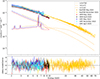 |
Fig. 3. Spectra from NuSTAR, XMM, and IXPE I, collected in May 2022, November 2022, and April 2025 for MCG-05-23-16, along with the best-fit model components for each instrument (shown only for the May 2022 campaign, when the source was observed simultaneous by all three instruments) and the residuals from the broadband (2–79 keV) spectral analysis in Sect. 3.2. Photon counting detector modules from NuSTAR (FPMA and FPMB) and IXPE DUs from the same campaign are grouped together for visual clarity. |
Best-fit parameters from the broadband spectral analysis of MCG-05-23-16 using NuSTAR (3–79 keV), XMM-Newton (2–10 keV), and IXPE I (2–8 keV) combined datasets.
In the final step of this broadband spectral analysis, we replaced zcutoffpl with the analytic Comptonization model compTT (Titarchuk 1994). We fixed the thermal photon temperature to 30 eV, which is appropriate for an AGN accretion disk and which only minimally affects the output spectrum (Schneider et al. 2013). We also fixed the reflection parameters to the values previously determined. Assuming a slab geometry for the corona, we obtain a coronal temperature kTe = 36 ± 2 keV and a coronal optical depth τ = 1.1 ± 0.1. In contrast, assuming a more spherical geometry, we retrieve kTe = 33 ± 2 keV and τ = 3.0 ± 0.2. These measurements are consistent (within 3σ) with previous inferences (Baloković et al. 2015; Marinucci et al. 2022; Serafinelli et al. 2023). Fig. 4 shows the spectra used for this final spectral analysis, together with the model components for each instrument (shown only for the May 2022 campaign, when the source was observed simultaneously by the three instruments) and the residuals.
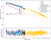 |
Fig. 4. Same as Fig. 3, but using compTT (assuming a slab coronal configuration) instead of cutoffpl. |
3.3. Broadband spectropolarimetric analysis
Next, we assigned a distinct polarization signature to each model component using the convolutive polarization kernel polconst in XSPEC. Because the Fe Kα line is expected to be intrinsically unpolarized (Goosmann & Matt 2011; Marin et al. 2018), and the Compton reflection component contributes only marginally to the IXPE energy band (Marin et al. 2018), we initially fixed the polarization degree of both relxill and xillver to zero. We allowed only the polarization properties of the primary continuum to vary.
The overall fit is acceptable, with χ2/d.o.f. = 3083/2879. Given the absence of significant residuals and the complexity of combining multiple instruments across different epochs, we attribute the residuals to cross-calibration systematics, as already discussed by Tagliacozzo et al. (2023). From this combined analysis, we obtained only an upper limit at the 99% confidence level on the primary continuum polarization, with P < 2.8%. As for the previous observations, although the polarization angle is unconstrained and we lack a definitive polarization detection, our analysis suggests a statistical tendency for the polarization angle to lie between 20° and 70° (see the left panel of Fig. 2).
Next, we performed a series of tests by assigning different polarization degrees and angles to the reflection components (i.e., relxill and xillver) relative to the primary continuum component (cutoffpl). To assess the contribution of the Fe Kα line (likely unpolarized) relative to the reflection continuum, we replaced the xillver component with pexriv (Magdziarz & Zdziarski 1995) plus a Gaussian line. The line has a small equivalent width of  eV and a flux less than 1% of the total reflection flux in the IXPE energy range (i.e., 2–8 keV), resulting in no significant impact on the polarization constraints. Among these tests, summarized in Table 3 and similar to those of Gianolli et al. (2023), we forced the polarization of the reflection components to be perpendicular to that of the primary continuum and assumed physically motivated values of P (Marin et al. 2018). In particular, we tested Pxillver = Prelxill = 10, 20, and 30%. Because the overall 2–8 keV polarization is notably low, as indicated by our model-independent analysis (see Sect. 3.1), assuming highly polarized reflected radiation naturally implies a correspondingly higher polarization of the primary continuum (assumed to be perpendicular to the reflection), consistent with expectations for this scenario.
X-ray polarimetry of MCG-05-23-16 from model-dependent analyses.
As a result, we obtained only an upper limit at the 99% confidence level on Ppl (< 4%) for Pxillver = Prelxill = 10%. When assuming a higher polarization for the reflected components, we measured Ppl = (2.2 ± 0.7)% at the 68% confidence level for Pxillver = Prelxill = 20%, and Ppl = (3.7 ± 0.7)% for Pxillver = Prelxill = 30%, indicating a consistent increase in inferred continuum polarization. These spectropolarimetric tests suggest that the observed signal can be reproduced either by weakly polarized X-ray reflection (≤10%), implying a low intrinsic polarization of the primary continuum (≤4%), or by a scenario in which a more strongly polarized reflection (≥20%) is oriented nearly orthogonally to a few-percent polarized continuum, leading to partial cancelation of the net signal. The latter scenario requires specific scattering geometries.
4. Comparison to simulations
To interpret our measurements, we explored the possible shape and location of the X-ray corona using Monte Carlo simulations. We used the MONK code, a Monte Carlo radiative transfer code designed to calculate Comptonized spectra in the Kerr spacetime (Zhang et al. 2019).
We simulated a series of X-ray coronae of different shapes and locations, following the approaches of Ursini et al. (2022), Gianolli et al. (2023), Tagliacozzo et al. (2023), Ingram et al. (2023), and Chakraborty et al. (2025). We focused on the four most common and probable coronal configurations:
-
Aspherical lamppost corona. This configuration consists of a spherical, compact, stationary source located along the disk axis. Its size depends on the spin of the supermassive black hole. It tends to produce reflection-dominated spectra in AGN (Matt et al. 1991; Martocchia & Matt 1996; Petrucci & Henri 1997; Wilkins & Fabian 2012; Ursini et al. 2020a, 2022);
-
Conical outflows. They consist of a conical mass located along the symmetry axis of the accretion disk and are commonly associated with an aborted jet. In this model, radio-quiet AGNs host a central supermassive black hole that powers outflows and jets, which propagate only over short distances if the velocity of the ejected material is subrelativistic and lower than the local escape velocity. Consequently, the material travels only up to a limited distance before falling back and colliding with subsequent blobs. This process results in the dissipation of kinetic energy and the production of high-energy emission in these objects (Petrucci & Henri 1997; Ghisellini et al. 2004; Ursini et al. 2022);
-
Aslab corona. In this scenario, the hot medium is assumed to be uniformly distributed above the disk. This geometry can result from magnetic loops rising high above the disk plane and dissipating energy through reconnection. Energy dissipation and electron heating occur throughout a large volume, and the corona is assumed to co-rotate with the Keplerian disk (Liang 1979; Haardt & Maraschi 1991; Beloborodov 2017);
-
A wedge corona. This configuration resembles the slab geometry, but has a height that increases with radius. In this scenario, the disk is thought to be truncated at a certain radius, while the corona represents a form of “hot accretion flow”, possibly extending to the ISCO (see Esin et al. (1997), Schnittman & Krolik (2010), Marcel et al. (2018), Poutanen et al. (2018), Ursini et al. (2020b), Tagliacozzo et al. (2025)).
We performed MONK simulations for a total of 24 parameter combinations. For the lamppost and slab cases, we simulated two spin configurations (null and maximum), for two disk radii: 25 RG and the ISCO, which corresponds to 6 RG for the null spin case and 1.24 RG for the maximum spin case. For the wedge case, we simulated four different coronal openings (15°, 30°, 45°, and 60°), for each spin and radius described above. For the conical case, we adopted the results from Ursini et al. (2022), who simulated three different configurations: maximum spin with a disk-plane height d = 3 RG and vertical thickness t = 10 RG, null spin with d = 5 RG and t = 15 RG, and null spin with d = 20 RG and t = 20 RG. Because the MONK simulations in Ursini et al. (2022) were performed with a coronal electron temperature of 25 keV, we adopted the same value, which is also consistent with our own values derived in Sect. 3.2 and with those reported by Baloković et al. (2015). However, given the degeneracy between kTe and τ for a fixed spectral slope, a slight increase in kTe does not cause a significant variation in the expected polarization properties of the source, as found, for example, by Tagliacozzo et al. (2025). For each geometric configuration, we determined the optical depth that best reproduces the observed spectrum in the IXPE bandpass (2–8 keV), by replacing the cutoff power-law component with spectra generated by MONK within the best-fit model from Sect. 3.2. We assumed a supermassive black hole mass of MBH = 2 × 10⁷ M⊙ and an Eddington ratio of 0.1 for all simulations (Ponti et al. 2012). Finally, we set the initial polarization, defined as the polarization of the optical and ultraviolet radiation emitted by the accretion disk, to values appropriate for a pure scattering, plane-parallel, semi-infinite atmosphere (Chandrasekhar 1960).
We found polarization angles parallel to the accretion disk axis in the slab and wedge cases, as expected. Conversely, for the lamppost and conical cases, we find angles perpendicular to the accretion disk axis. The polarization degree is highest for the slab geometry, lowest for the lamppost, and intermediate for the wedge and conical coronas. In the lamppost scenario, P remains below 1.5%. For the conical case, the configuration with null spin, d = 20 RG, and t = 20 RG yields the highest P (up to 6%). The slab corona cases with null spin produce lower P (up to 7%), whereas cases with maximum spin produce higher P (up to 13%). In the wedge scenario, previously investigated by Tagliacozzo et al. (2025), P is maximum for lower opening angles and higher black hole spins.
Figures 5 and 6 show the polarization degree P as a function of the cosine of the system inclination angle, cos(θdisk). Because all models are axisymmetric, P is lowest at cos(θdisk) = 1 (face-on view) and highest at cos(θdisk) = 0 (edge-on view). The green regions represent the allowed values of the polarization degree: pale green indicates the constraint on P derived from the broadband spectropolarimetric analysis in Sect. 3.3, while saturated green shows the combination of constraints on P and the system inclination (29° < θdisk < 66°) from a conservative combination of estimates across various wavebands (see Sect. 5.3). Comparison of our simulations with the data analysis results shows that the lamppost model is compatible with all tested scenarios, similar to the conical corona configuration, except for the case with d = 20 RG and t = 20 RG. Both models predict polarization angles perpendicular to the disk axis, with stringent upper limits (P ≤ 1.1%). The slab geometry yields polarization degrees compatible with the constraints, whereas the wedge model is compatible in most cases. Both models predict polarization angles parallel to the disk axis, with an effective polarization upper limit of 2.4%. In summary, the combination of the inclination estimates and the upper limits on the polarization fraction lead to the inability to distinguish between different coronal models.
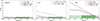 |
Fig. 5. Polarization degree from MONK simulations as a function of the cosine of the system inclination angle cos(θdisk) for a spherical lamppost model (left panel), a conical outflows model (middle panel), and a slab corona model (right panel). The cases cos(θdisk) = 0 and cos(θdisk) = 1 represent the edge-on and face-on views of the source, respectively. The green regions indicate the allowed values of the polarization degree: pale green represents the constraint on P from the broadband spectropolarimetric analysis in Sect. 3.3, while saturated green represents the combination of the constraints on P and the system inclination (Sect. 5.3). Because the lamppost and conical geometries yield θ perpendicular to the accretion disk axis, the resulting polarization constraint is set to P < 1.1% in the left and middle panels. Conversely, the slab geometry yields θ parallel to the disk, with P < 2.4%. |
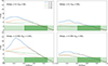 |
Fig. 6. Same as in Fig. 5, but shown only for the wedge corona model. This geometry, like the slab, yields θ parallel to the disk, leading to P < 2.4%. |
5. Interpretation of our X-ray results in the context of near-ultraviolet to near-infrared (spectro)polarimetry
Taken at face value, our X-ray polarimetric results either disfavor equatorial coronal geometries (slab or wedge) if the inclination of MCG–5–23–16 is large, as previously estimated, or indicate that the orientation of the AGN core is relatively low, in contradiction with its type 1.9 classification. To break this degeneracy, we used an unpublished optical spectropolarimetric observation of MCG–5–23–16 obtained with the FOcal Reducer/low dispersion Spectrograph 2 (FORS2) mounted on the Very Large Telescope (VLT).
5.1. Data reduction
The data were acquired on May 12, 2019 with the Unit 1 (Antu) telescope, during Program ID 0101.B-0530(A). A Wollaston prism splits the incoming light into two orthogonally polarized beams separated by 22″ on the CCD. To measure the normalized Stokes parameters q and u, we took four 200 s exposures with the half-wave plate rotated to 0°, 22.5°, 45°, and 67.5°, minimizing instrumental polarization. We recorded spectra with the 300V grism and GG435 filter, covering 4600–8650 Å. A 1″ slit provided a resolving power of R ≈ 440 at 5849 Å, sufficient to sample broad emission lines. The slit was oriented along the parallactic angle. We binned the CCD pixels 2 × 2 (0.25″ per pixel). The total exposure time was 800 s, the airmass remained constant during the observation (around 1.04) and the seeing was about 0.95″. We observed polarized and unpolarized standards (Fossati et al. 2007): Vela1-95 (April 1), Hiltner 652 (July 26 and August 28), HD 42078 (April 1), and WD 1620-391 (August 28). Instrumental polarization remained below 0.1%.
We cleaned waw frames of cosmic rays using the Python implementation of lacosmic (van Dokkum 2001; van Dokkum et al. 2012). We reduced the data using the European Southern Observatory (ESO) FORS2 pipeline (Izzo et al. 2019), which yielded flat-fielded, rectified, and wavelength-calibrated spectra. We extracted one-dimensional spectra with a 1.75″ (7-pixel) aperture, minimizing host contamination while retaining flux. We extracted sky spectra from adjacent MOS strips and subtracted them. We computed the Stokes parameters from the ordinary and extraordinary beams following the FORS2 manual1, correcting for the chromatic dependence of the half-wave plate. We corrected the fluxes for atmospheric extinction and calibrated them using a master response curve. We derived uncertainties by propagating photon and readout noise. We obtained the polarization degree P and angle θ following the same procedure as for the X-ray polarization measurements presented earlier in this paper.
5.2. Analysis
We present the results of this observation in Fig. 7. The total flux spectrum is shown at native spectral resolution; however, because the polarization is too noisy (see Fig. B.1 in the appendices for the unbinned version), we binned the polarized spectra so that each spectral bin has a polarization S/N of at least three. The total flux spectrum shows only narrow emission lines on top of a reddened continuum, a spectral shape long established in the literature (see, e.g. Lumsden et al. 2004). We fit the main Balmer lines and found a full width at half maximum (FWHM) of about 410 km s−1 for Hα and about 330 km s−1 for Hβ. However, the unbinned polarized flux shows a larger Hα line, with FWHM ∼ 2250 km s−1, and no detectable Hβ emission (see Fig. B.1). The Hα FWHM we find is comparable to the ∼2150 km s−1 quoted by Blanco et al. (1990) for Brγ, indicating that both emission lines share a common physical origin. The polarized continuum is significantly redder than the total flux, indicating that the polarized light is affected by substantial dust extinction, which preferentially suppresses the blue wavelengths. The polarization degree (Fig. 7, bottom-left panel) shows a similar trend, with P on the order of 0.25% around 5000 Å, a peak at the location of the Hα line, and a rise toward 9000 Å, reaching up to 1%. Remarkably, the chromaticity of P is closely coupled to a rotation of the polarization angle from about 100° in the blue band to ∼30° longward of Hα, where θ stabilizes toward the end of the red band. The combination of those two independent quantities points toward a change in the polarization mechanism between the two ends of the spectrum. To investigate this, we first checked whether our data are contaminated by interstellar polarization (ISP), that is, by the effect of Milky Way’s dust and magnetized interstellar medium. For this purpose, we used the compilation of optical starlight polarization catalogs presented by Panopoulou et al. (2025) and selected the closest star with available polarimetric measurements: GaiaDR2 3244105248118361984. This star lies 2.27° from MCG-5-23-16, with polarization P = 0.25% ± 0.1% at θ = 39.1° ± 12.8°. While the measured red-band polarization in MCG-5-23-16 exceeds the ISP value by 0.72% ± 0.12%, corresponding to a significance of about 5.8σ, the blue band shows a similar polarization level but with a different polarization angle. This suggests that ISP may contribute to the observed polarization in the blue band, with dichroic absorption dominating the production of polarization, overlaid with a second component that drives the rotation of θ.
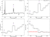 |
Fig. 7. Spectropolarimetry of MCG-5-23-16 obtained with VLT/FORS2. Top-left panel: Total flux spectrum, corrected for the instrumental response (in arbitrary units). Top-right panel: Polarized flux, obtained by multiplying the total flux by the polarization degree. Bottom-left panel: Linear polarization degree. Bottom-right panel: Polarization position angle. Except for the total flux panel, spectra were rebinned to 137 consecutive pixels (424.8 Å) to achieve a polarization S/N of at least three per bin. Observational errors are shown for each spectral bin. The newly estimated position angle of the extended [O III] and Hα emission line region from (Ferruit et al. 2000) is indicated with a dashed red line in the polarization angle panel. |
We then compared our data with previous polarimetric measurements to verify whether they agree and if the chromaticity in P and θ extends to shorter and longer wavelengths. Few polarimetric observations of this source exist in the literature: two papers report broadband polarimetry (Martin et al. 1983; Brindle et al. 1990) and one paper presents spectropolarimetry (Lumsden et al. 2004). The latter data were of lower S/N and added little new information; therefore, in Fig. 8, we superimposed only the broadband U, R, J, and H polarimetric points of Brindle et al. (1990) and the Coming 4-96 filter (3800–5600 Å) measurement of Martin et al. (1983) on our data, noting that these observations were obtained with larger apertures (between 4″ and 6″) and under different observing conditions than ours. Nevertheless, the results agree well with ours, both in terms of P and θ. The polarization of this source appears to have remained unchanged for decades. More importantly, the U-band polarimetric point of Brindle et al. (1990) confirms the rotation of the polarization angle at short wavelengths, with a value of 132° ± 17°, that is, orthogonal to the polarization angle in the red band. The J- and H-band polarization angles confirm that θ remains stable, at least up to 1.8 μm. The polarization degree in the infrared also appears to stabilize, at about 0.8%, which is consistent with our red band measurement within the uncertainties.
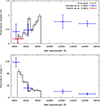 |
Fig. 8. Spectropolarimetric results compared to the broadband measurements of Martin et al. (1983) (red) and Brindle et al. (1990) (blue). The polarization angle is unconstrained in the single measurement of Martin et al. (1983). |
With all this information in hand, we next examine the alignment between the polarization position angle and the radio jet or AGN outflows axes to determine the wavelength-dependent polarization of MCG-5-23-16 in the optical and the nondetection of its X-ray polarized counterpart. This test was established for radio galaxies by Antonucci (1983), then for Seyfert galaxies, and finally extended to all nonblazing AGNs (Antonucci 1993). Comparing the two provides insight into the global AGN orientation and helps identify whether the regions responsible for the observed polarization are equatorial or polar. The position angle of the radio jet structure in MCG-5-23-16 remains uncertain because it is only marginally resolved in 1.4 GHz Karl G. Jansky Very Large Array (VLA) images obtained by Mundell et al. (2009) (see also Orienti & Prieto (2010)). The estimated position angle of the radio structure is approximately −11°, which is neither parallel nor perpendicular to the optical polarization angle in either the blue or red bands. In the absence of a clear radio structure, it is common to look at the position angle of the AGN ionization axes, highlighted in the optical and infrared bands by their emission line outflows. Previous observations revealed that the [O III] emission in MCG-5-23-16 is elongated on either side of the nucleus at a position angle of 40°, uncorrelated with the marginally extended radio emission (Ferruit et al. 2000). If we take this value as the reference angle for comparison with our polarization angle (26° ± 2° at 8424 Å), the two appear nearly aligned but differ by ∼14°, corresponding to a > 6σ discrepancy when accounting for the modulo-180° ambiguity.
To better understand the underlying situation, we carefully examined the extension and position angle of the outflows, as revealed by their line emission in Ferruit et al. (2000). Figure 9 shows a digitized reproduction of their color map of MCG-5-23-16, taken with the Wide Field and Planetary Camera 2 (WFPC2) onboard the Hubble Space Telescope (HST), with their [O III] λ5007 image superposed. We emphasize that we did not re-reduce the data, but simply extracted their published figure. For reference, we indicate the position angle of the radio jet axis originally estimated by Mundell et al. (2009) in pink. In yellow, we show the position angle of the [O III] region, measured by identifying the direction of maximum spatial extension of the forbidden emission above a given surface-brightness threshold. The position angle corresponds to the vector that joins the nucleus with the most distant pixel within the contiguous emission region in the south-west quadrant. Our measurement2 yields a position angle of 28° ± 4°, which differs from the value proposed by Ferruit et al. (2000). The value reported by the authors (40°) instead corresponds to a more marginal extension in the opposite quadrant – the north-east one – which could be distorted by the presence of an emission blob, as suggested by the shape of the isophotes. For this extension, we measured a position angle of 43° ± 6°. However, this value conflicts with the presence of an optically thick dust lane observed in projection crossing very close to the AGN center, at a position angle of about 46° (Prieto et al. 2014), shown in red in Fig. 9. This dust lane, which is part of a much larger kiloparsec-scale structure (Prieto et al. 2014), is either an isolated filament or the edge-on disk of the host galaxy itself (Esparza-Arredondo et al. 2025). In any case, the [O III] outflow in this quadrant is almost certainly partially obscured by dust, and its position angle must therefore be considered as highly uncertain. For this reason, we focus on the less dust-affected south-west quadrant.
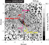 |
Fig. 9. Color map of MCG-5-23-16 from HST/WFPC2, extracted from Ferruit et al. (2000) (see their Fig. 8). North is up and east is to the left. The map was constructed by dividing the F547M continuum image by the F791W image and taking the logarithm. Darker regions (lower values of log (F547M/F791W)) correspond to redder areas. Selected isophotes (8, 16, 64, and 256 × 10−15 ergs s−1 cm−2 arcsec−2) of the [O III] λ5007 image are superposed on the image. The gray scales are linear and the pixel size is 0.0996 arcsec−2. The pink line indicates the position angle of the radio-jet axis, marginally measured by Mundell et al. (2009) and Orienti & Prieto (2010), traced on top of the image from Ferruit et al. (2000). The red line shows our measured position angle of the dust lane extracted from Prieto et al. (2014). The yellow line marks our new estimation of the position angle of the maximal extension of the [O III] λ5007 emission. |
Accounting for the dust lane, the observational pieces align. The position angle of the AGN ionization axis becomes parallel to the near-infrared and infrared polarization (shown in red in the bottom-right panel of Fig. 7) and perpendicular in the blue band. In the infrared, dust extinction from the filament is weaker, allowing us to directly observe the core emission of MCG-5-23-16, including the broad Paβ emission from the broad line region (BLR; see Goodrich et al. (1994)). Toward the optical band, dust extinction increases (as highlighted by the shape of the polarized flux; Fig. 7, top-right panel), so photons reach the observer only after scattering off the polar outflows. This explains why we observe Hα in polarized light only. Because optical core photons are scattered perpendicularly in the narrow line region (NLR), the polarization angle rotates, reaching an orthogonal value shortward of Hα. The decrease in P toward the blue part of our spectrum results from a combination of starlight and ISP, which cancels the small polarized flux from core AGN photons scattered off the NLR. This explains the nondetection of the broad Hβ line (further compounded by the lower S/N in the blue). The observed variety of detections and nondetections of broad lines across the blue, optical, and infrared bands arises because the true cause of the nucleus obscuration is not the usual optically thick, compact, circumnuclear reservoir of dust and gas (the torus), but the less-dense, distant dust lane bisecting the galaxy. This implies that MCG–5-23-16 is not intrinsically a type 1.9/2 AGN; it is a type 1 nucleus viewed through a foreground dust lane that is unrelated to the AGN itself. This also explains the low hydrogen column density toward MCG-5-23-16 (nH ≈ 1022 at cm−2; see Sect. 3.2), its lack of significant variation over decades (consistent with an obscurer on kiloparsec scales; Serafinelli et al. 2023), and why MCG-05-23-16 continues to elude X-ray polarimetric detection. Its accretion structure, hot corona, and BLR are seen almost face-on, yielding a very low expected X-ray polarization degree, even for equatorial models (see Fig. 6 and Tagliacozzo et al. 2025).
5.3. The true orientation of the nucleus of MCG-05-23-16
The idea that obscuration in some Seyfert galaxies arises primarily from a host-galaxy dust lane rather than from a compact torus has been discussed in the literature (e.g., Maiolino & Rieke 1995; Matt 2000; Bianchi et al. 2012). Our results provide compelling evidence that this is also the case for MCG-05-23-16 (Prieto et al. 2014). The Seyfert galaxy is, in fact, a type 1 AGN unintentionally disguised as a type 1.9/2 AGN. This also explains why it has been so difficult to estimate its core orientation.
Using Advanced Satellite for Cosmology and Astrophysics (ASCA) data, Turner et al. (1998) fit the iron Kα line on top of a single power-law continuum in a relativistic framework and estimated the inclination of the accretion disk in MCG-05-23-16 to be 33 . Weaver et al. (1997) found a larger inclination using the same methodology (about 65°), likely due to the assumptions made in the fit. Reeves et al. (2007) modeled the Suzaku X-ray spectrum of this source using a combination of reflection from both distant matter and the accretion disk, and determined that the most probable inclination of MCG-05-23-16 is ∼50°. Simultaneous deep XMM-Newton and Chandra observations of MCG-5-23-16 enabled Braito et al. (2007) to achieve a time-averaged spectral analysis of the iron K-shell complex, which is well described by an emission line originating from an accretion disk viewed with an inclination angle of about 40°. Taking advantage of the first contemporaneous X-ray observation of this AGN by XMM-Newton and NuSTAR, Serafinelli et al. (2023) analyzed the shape of the broad iron line and determined an inclination of 41
 . Using a different technique, Fuller et al. (2016) compiled infrared fluxes of MCG-05-23-16 and used numerical torus models together with a Bayesian approach to fit its infrared nuclear spectral energy distribution, constraining the torus inclination to 62
 . Even in our own broadband analysis (see Sect. 3.2), θincl is unbound unless constrained prior to the fit.
Depending on the waveband, model, and assumptions, the estimated inclination of MCG-05-23-16 ranges from 29° to 66°, according to the cited studies. Determining the orientation of an AGN core is extremely difficult, and no single method yields consistent results across a large test sample (Marin 2016). One possible explanation for this discrepancy is that MCG-05-23-16 was initially considered a type 1.9/2 AGN based solely on its optical and near-infrared spectra. This optical classification naturally led some authors to favor models with higher inclinations (e.g., Weaver et al. 1997). Now that MCG-05-23-16 is recognized as a type 1 AGN viewed through a foreground dust lane, future modeling can be performed without this assumption, enabling a more reliable reassessment of its inclination.
6. Conclusions
In this paper, we report the third IXPE pointing of MCG-05-23-16, together with new optical spectropolarimetry obtained with the VLT, combined with archival near-ultraviolet, optical, and near-infrared polarimetric data. No polarization was detected in the 2–8 keV energy range, with an upper limit of ≤2.9% (99% confidence level). Combining the new IXPE pointing with the previous two (May and November 2022) reduced the upper limit to ≤2.5% (99% confidence level). Monte Carlo simulations of the X-ray corona indicate that equatorial models (slab or wedge) are disfavored if the AGN is highly inclined, as suggested by its historical type 1.9/2 classification. However, a corona coplanar with the accretion disk remains a viable solution if the source is less inclined than usually assumed.
To determine which of the two scenarios is the correct one, we analyzed a 2019 VLT/FORS2 dataset to obtain optical and near-infrared spectropolarimetry of the source. The total flux spectrum displays only narrow emission lines superimposed on a reddened continuum, consistent with a Seyfert-2/1.9 classification. However, the polarized spectrum reveals a broad Hα in scattered light and a strong wavelength dependence of both the polarization degree and angle, with a rotation of nearly 70° between the blue and red bands. Comparison with historical near-ultraviolet, optical, and infrared measurements demonstrates (1) long-term stability of the polarization spectrum, pointing to a persistent mechanism, and (2) that the rotation of the polarization angle reaches 90° in the U-band.
After defining the proper reference for comparing our polarization data, namely the ionization axis of the AGN, we show that the observed polarization is best explained by a type 1 nucleus viewed through a large-scale, distant, and moderately obscuring dust lane rather than by an optically thick, compact, and circumnuclear torus. This reinterpretation explains why the source has such a moderate hydrogen column density for an AGN previously thought to be strongly inclined. This is consistent with the absence of an X-ray polarimetric detection by IXPE, since the source is effectively a face-on type 1 AGN whose hot corona yields intrinsically low X-ray polarization. Our results remove MCG-05-23-16 from the sample of bona fide Seyfert-1.9 galaxies and call for a reassessment of its orientation using models not biased by this long-standing misclassification.
Acknowledgments
The Imaging X ray Polarimetry Explorer (IXPE) is a joint US and Italian mission. The US contribution is supported by the National Aeronautics and Space Administration (NASA) and led and managed by its Marshall Space Flight Center (MSFC), with industry partner Ball Aerospace (contract NNM15AA18C). The Italian contribution is supported by the Italian Space Agency (Agenzia Spaziale Italiana, ASI) through contract ASI-OHBI-2022-13-I.0, agreements ASI-INAF-2022-19-HH.0 and ASI-INFN-2017.13-H0, and its Space Science Data Center (SSDC) with agreements ASI-INAF-2022-14-HH.0 and ASI-INFN 2021-43-HH.0, and by the Istituto Nazionale di Astrofisica (INAF) and the Istituto Nazionale di Fisica Nucleare (INFN) in Italy. This research used data products provided by the IXPE Team (MSFC, SSDC, INAF, and INFN) and distributed with additional software tools by the High-Energy Astrophysics Science Archive Research Center (HEASARC), at NASA Goddard Space Flight Center (GSFC). This work made use of data supplied by the UK Swift Science Data Centre at the University of Leicester. DH is research director at the F.R.S-FNRS, Belgium. V.E.G. acknowledges funding under NASA contract 80NSSC24K1403. POP acknowledges financial support from the french national space agency (CNES) and the CNRS ATPEM. R.S. acknowledges funding from the CAS-ANID grant number CAS220016. J.S. thanks GACR project 21-06825X for the support. D.H. is F.R.S-FNRS research director (Belgium).
References
- Antonucci, R. R. J. 1983, Nature, 303, 158 [NASA ADS] [CrossRef] [Google Scholar]
- Antonucci, R. 1993, ARA&A, 31, 473 [Google Scholar]
- Arnaud, K. A. 1996, in Astronomical Data Analysis Software and Systems V, eds. G. H. Jacoby, & J. Barnes, ASP Conf. Ser., 101, 17 [NASA ADS] [Google Scholar]
- Baloković, M., Matt, G., Harrison, F. A., et al. 2015, ApJ, 800, 62 [CrossRef] [Google Scholar]
- Beloborodov, A. M. 2017, ApJ, 850, 141 [NASA ADS] [CrossRef] [Google Scholar]
- Bianchi, S., Maiolino, R., & Risaliti, G. 2012, Adv. Astron., 2012, 782030 [CrossRef] [Google Scholar]
- Blanco, P. R., Ward, M. J., & Wright, G. S. 1990, MNRAS, 242, 4P [Google Scholar]
- Braito, V., Reeves, J. N., Dewangan, G. C., et al. 2007, ApJ, 670, 978 [NASA ADS] [CrossRef] [Google Scholar]
- Brindle, C., Hough, J. H., Bailey, J. A., et al. 1990, MNRAS, 244, 577 [NASA ADS] [Google Scholar]
- Chakraborty, S., Ratheesh, A., Tagliacozzo, D., et al. 2025, ApJ, 990, 89 [Google Scholar]
- Chandrasekhar, S. 1960, Radiative Transfer (New York: Dover) [Google Scholar]
- Di Marco, A., Costa, E., Muleri, F., et al. 2022, AJ, 163, 170 [NASA ADS] [CrossRef] [Google Scholar]
- Di Marco, A., Soffitta, P., Costa, E., et al. 2023, AJ, 165, 143 [CrossRef] [Google Scholar]
- Esin, A. A., McClintock, J. E., & Narayan, R. 1997, ApJ, 489, 865 [NASA ADS] [CrossRef] [Google Scholar]
- Esparza-Arredondo, D., Ramos Almeida, C., Audibert, A., et al. 2025, A&A, 693, A174 [NASA ADS] [CrossRef] [EDP Sciences] [Google Scholar]
- Ferruit, P., Wilson, A. S., & Mulchaey, J. 2000, ApJS, 128, 139 [Google Scholar]
- Fossati, L., Bagnulo, S., Mason, E., & Landi Degl’Innocenti, E. 2007, in The Future of Photometric, Spectrophotometric and Polarimetric Standardization, ed. C. Sterken, ASP Conf. Ser., 364, 503 [Google Scholar]
- Fuller, L., Lopez-Rodriguez, E., Packham, C., et al. 2016, MNRAS, 462, 2618 [NASA ADS] [CrossRef] [Google Scholar]
- Gabriel, C., Denby, M., Fyfe, D. J., et al. 2004, in Astronomical Data Analysis Software and Systems (ADASS) XIII, eds. F. Ochsenbein, M. G. Allen, & D. Egret, ASP Conf. Ser., 314, 759 [NASA ADS] [Google Scholar]
- Ghisellini, G., Haardt, F., & Matt, G. 2004, A&A, 413, 535 [NASA ADS] [CrossRef] [EDP Sciences] [Google Scholar]
- Gianolli, V. E., Kim, D. E., Bianchi, S., et al. 2023, MNRAS, 523, 4468 [NASA ADS] [CrossRef] [Google Scholar]
- Gianolli, V. E., Bianchi, S., Kammoun, E., et al. 2024, A&A, 691, A29 [NASA ADS] [CrossRef] [EDP Sciences] [Google Scholar]
- Goodrich, R. W., Veilleux, S., & Hill, G. J. 1994, ApJ, 422, 521 [NASA ADS] [CrossRef] [Google Scholar]
- Goosmann, R. W., & Matt, G. 2011, MNRAS, 415, 3119 [NASA ADS] [CrossRef] [Google Scholar]
- Haardt, F., & Maraschi, L. 1991, ApJ, 380, L51 [Google Scholar]
- HI4PI Collaboration (Ben Bekhti, N., et al.) 2016, A&A, 594, A116 [NASA ADS] [CrossRef] [EDP Sciences] [Google Scholar]
- Ingram, A., Ewing, M., Marinucci, A., et al. 2023, MNRAS, 525, 5437 [CrossRef] [Google Scholar]
- Izzo, C., de Bilbao, d. B., & Larsen, J. 2019, FORS Pipeline User Manual, VLT-MAN-ESO-19500-4106 [Google Scholar]
- Krawczynski, H., Muleri, F., Dovčiak, M., et al. 2022, Science, 378, 650 [NASA ADS] [CrossRef] [Google Scholar]
- Liang, E. P. T. 1979, ApJ, 231, L111 [Google Scholar]
- Lumsden, S. L., Alexander, D. M., & Hough, J. H. 2004, MNRAS, 348, 1451 [Google Scholar]
- Magdziarz, P., & Zdziarski, A. A. 1995, MNRAS, 273, 837 [Google Scholar]
- Maiolino, R., & Rieke, G. H. 1995, ApJ, 454, 95 [Google Scholar]
- Marcel, G., Ferreira, J., Petrucci, P.-O., et al. 2018, A&A, 617, A46 [NASA ADS] [CrossRef] [EDP Sciences] [Google Scholar]
- Marin, F. 2016, MNRAS, 460, 3679 [CrossRef] [Google Scholar]
- Marin, F., Dovčiak, M., & Kammoun, E. S. 2018, MNRAS, 478, 950 [NASA ADS] [CrossRef] [Google Scholar]
- Marinucci, A., Muleri, F., Dovciak, M., et al. 2022, MNRAS, 516, 5907 [NASA ADS] [CrossRef] [Google Scholar]
- Martin, P. G., Thompson, I. B., Maza, J., & Angel, J. R. P. 1983, ApJ, 266, 470 [CrossRef] [Google Scholar]
- Martocchia, A., & Matt, G. 1996, MNRAS, 282, L53 [NASA ADS] [CrossRef] [Google Scholar]
- Matt, G. 2000, A&A, 355, L31 [NASA ADS] [Google Scholar]
- Matt, G., Perola, G. C., & Piro, L. 1991, A&A, 247, 25 [NASA ADS] [Google Scholar]
- Mattson, B. J., & Weaver, K. A. 2004, ApJ, 601, 771 [Google Scholar]
- Miniutti, G., & Fabian, A. C. 2004, MNRAS, 349, 1435 [NASA ADS] [CrossRef] [Google Scholar]
- Mundell, C. G., Ferruit, P., Nagar, N., & Wilson, A. S. 2009, ApJ, 703, 802 [Google Scholar]
- Orienti, M., & Prieto, M. A. 2010, MNRAS, 401, 2599 [NASA ADS] [CrossRef] [Google Scholar]
- Panopoulou, G. V., Markopoulioti, L., Bouzelou, F., et al. 2025, ApJS, 276, 15 [NASA ADS] [CrossRef] [Google Scholar]
- Petrucci, P. O., & Henri, G. 1997, A&A, 326, 99 [NASA ADS] [Google Scholar]
- Piconcelli, E., Jimenez-Bailón, E., Guainazzi, M., et al. 2004, MNRAS, 351, 161 [Google Scholar]
- Ponti, G., Papadakis, I., Bianchi, S., et al. 2012, A&A, 542, A83 [NASA ADS] [CrossRef] [EDP Sciences] [Google Scholar]
- Poutanen, J., Veledina, A., & Zdziarski, A. A. 2018, A&A, 614, A79 [NASA ADS] [CrossRef] [EDP Sciences] [Google Scholar]
- Prieto, M. A., Mezcua, M., Fernández-Ontiveros, J. A., & Schartmann, M. 2014, MNRAS, 442, 2145 [Google Scholar]
- Reeves, J. N., Awaki, H., Dewangan, G. C., et al. 2007, PASJ, 59, 301 [NASA ADS] [Google Scholar]
- Schneider, E. E., Impey, C. D., Trump, J. R., & Salvato, M. 2013, ApJ, 766, 123 [Google Scholar]
- Schnittman, J. D., & Krolik, J. H. 2010, ApJ, 712, 908 [NASA ADS] [CrossRef] [Google Scholar]
- Serafinelli, R., Marinucci, A., De Rosa, A., et al. 2023, MNRAS, 526, 3540 [NASA ADS] [CrossRef] [Google Scholar]
- Strohmayer, T. E. 2017, ApJ, 838, 72 [NASA ADS] [CrossRef] [Google Scholar]
- Strüder, L., Briel, U., Dennerl, K., et al. 2001, A&A, 365, L18 [Google Scholar]
- Tagliacozzo, D., Marinucci, A., Ursini, F., et al. 2023, MNRAS, 525, 4735 [CrossRef] [Google Scholar]
- Tagliacozzo, D., Bianchi, S., Gianolli, V., et al. 2025, A&A, 701, A241 [NASA ADS] [CrossRef] [EDP Sciences] [Google Scholar]
- Titarchuk, L. 1994, ApJ, 434, 570 [NASA ADS] [CrossRef] [Google Scholar]
- Turner, T. J., George, I. M., Nandra, K., & Mushotzky, R. F. 1998, ApJ, 493, 91 [Google Scholar]
- Turner, M. J. L., Abbey, A., Arnaud, M., et al. 2001, A&A, 365, L27 [CrossRef] [EDP Sciences] [Google Scholar]
- Ursini, F., Dovčiak, M., Zhang, W., et al. 2020a, A&A, 644, A132 [NASA ADS] [CrossRef] [EDP Sciences] [Google Scholar]
- Ursini, F., Petrucci, P.-O., Bianchi, S., et al. 2020b, A&A, 634, A92 [NASA ADS] [CrossRef] [EDP Sciences] [Google Scholar]
- Ursini, F., Matt, G., Bianchi, S., et al. 2022, MNRAS, 510, 3674 [NASA ADS] [CrossRef] [Google Scholar]
- van Dokkum, P. G. 2001, PASP, 113, 1420 [Google Scholar]
- van Dokkum, P. G., Bloom, J., & Tewes, M. 2012, L.A.Cosmic: Laplacian Cosmic Ray Identification, Astrophysics Source Code Library [record ascl:1207.005] [Google Scholar]
- Weaver, K. A., Yaqoob, T., Mushotzky, R. F., et al. 1997, ApJ, 474, 675 [Google Scholar]
- Weisskopf, M. C., Soffitta, P., Baldini, L., et al. 2022, J. Astron. Telescopes Instrum. Syst., 8, 026002 [NASA ADS] [Google Scholar]
- Wilkins, D. R., & Fabian, A. C. 2012, MNRAS, 424, 1284 [NASA ADS] [CrossRef] [Google Scholar]
- Zhang, W., Dovciak, M., & Bursa, M. 2019, ApJ, 875, 148 [NASA ADS] [CrossRef] [Google Scholar]
Although the measurement depends on the adopted surface-brightness threshold, we verified that varying this threshold within a reasonable range does not significantly affect the derived position angle. The position angle remains stable within 4° for all tested thresholds, indicating that the result is robust against the specific choice of contour level.
Appendix A: X-ray observations
In Fig. A.1 we show the light curves of the three X-ray observing campaigns of MCG-05-23-16 used in this work.
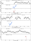 |
Fig. A.1. IXPE, NuSTAR and XMM-Newton light curves of the three observing campaigns of MCG-05-23-16 are shown. Except for the third IXPE observation, where we only had DU1 and DU3 available for the analysis, data counts from DU1, DU2 and DU3 on board of IXPE and from FPMA/A and FPMA/B on board of NuSTAR have been summed. The full energy bands of the three satellites have been used and we adopted a 3 ks time binning. |
Appendix B: Optical spectropolarimetry
In Fig. B.1, we present the unbinned total and polarized fluxes, the Q/I and U/I normalized Stokes parameters, and the polarization degree and angle of MCG-05-23-16 obtained with the grism 300V and the order-sorting filter GG435 with the VLT/FORS2. In contrast to Fig. 7, the polarized signal was not rebinned for the polarized counterpart. We thus observe the poor signal-to-noise ratio of the observation in polarization, that is particularly visible in the polarization angle panel. However, despite the statistical fluctuations, the broad Hα emission line is clearly visible in the Q/I, polarized flux, and polarization degree spectra. The width of the line is larger than in the optical, as already mentioned and measured by Lumsden et al. (2004). This observation confirms that the broad Hα line is indeed revealed in the polarized flux in MCG-05-23-16. No broad Hβ emission line is detected in the polarized flux spectrum, but it does not indicate that the line is absent. It could very well be hidden by bad statistics.
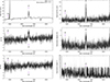 |
Fig. B.1. VLT/FORS2 spectropolarimetry of MCG-05-23-16. The top-left figure shows the total flux spectrum, corrected for the instrumental response (in arbitrary units). The middle- and bottom-left figures present the Q/I and U/I normalized Stokes parameters. The top-right panel shows the polarized flux, that is the multiplication of the total flux with the polarization degree. The middle-right panel presents the linear polarization degree while the bottom-right panel shows the polarization position angle. Spectra are shown at native spectral resolution. Observational errors are indicated in gray. |
For completeness, we also provide the polarization values of each of the spectral bins presented in Fig. 7 in Tab. B.1.
Optical polarization in the binned VLT/FORS2 spectrum.
All Tables
Best-fit parameters from the broadband spectral analysis of MCG-05-23-16 using NuSTAR (3–79 keV), XMM-Newton (2–10 keV), and IXPE I (2–8 keV) combined datasets.
All Figures
|
Fig. 1. Left panel: Stokes spectra Q (orange crosses) and U (magenta crosses) from the third IXPE pointing (April 2025) of MCG-05-23-16, shown with residuals and the corresponding best-fitting model. Right panel: Contour plot of the polarization degree P versus the polarization angle θ, summed over the 2 − 8 keV energy band of the third IXPE pointing. Purple, pink, and orange regions correspond to the 68%, 90%, and 99% confidence levels, respectively, for two parameters of interest. |
| In the text | |
|
Fig. 2. Contour plots of the polarization degree P and angle θ for the May 2022 observation (dotted contours), May 2022 and November 2022 (dashed contours), and for the May 2022, November 2022, and April 2025 observations combined (solid contours). Contours colors are the same as in Fig. 1. |
| In the text | |
|
Fig. 3. Spectra from NuSTAR, XMM, and IXPE I, collected in May 2022, November 2022, and April 2025 for MCG-05-23-16, along with the best-fit model components for each instrument (shown only for the May 2022 campaign, when the source was observed simultaneous by all three instruments) and the residuals from the broadband (2–79 keV) spectral analysis in Sect. 3.2. Photon counting detector modules from NuSTAR (FPMA and FPMB) and IXPE DUs from the same campaign are grouped together for visual clarity. |
| In the text | |
|
Fig. 4. Same as Fig. 3, but using compTT (assuming a slab coronal configuration) instead of cutoffpl. |
| In the text | |
|
Fig. 5. Polarization degree from MONK simulations as a function of the cosine of the system inclination angle cos(θdisk) for a spherical lamppost model (left panel), a conical outflows model (middle panel), and a slab corona model (right panel). The cases cos(θdisk) = 0 and cos(θdisk) = 1 represent the edge-on and face-on views of the source, respectively. The green regions indicate the allowed values of the polarization degree: pale green represents the constraint on P from the broadband spectropolarimetric analysis in Sect. 3.3, while saturated green represents the combination of the constraints on P and the system inclination (Sect. 5.3). Because the lamppost and conical geometries yield θ perpendicular to the accretion disk axis, the resulting polarization constraint is set to P < 1.1% in the left and middle panels. Conversely, the slab geometry yields θ parallel to the disk, with P < 2.4%. |
| In the text | |
|
Fig. 6. Same as in Fig. 5, but shown only for the wedge corona model. This geometry, like the slab, yields θ parallel to the disk, leading to P < 2.4%. |
| In the text | |
|
Fig. 7. Spectropolarimetry of MCG-5-23-16 obtained with VLT/FORS2. Top-left panel: Total flux spectrum, corrected for the instrumental response (in arbitrary units). Top-right panel: Polarized flux, obtained by multiplying the total flux by the polarization degree. Bottom-left panel: Linear polarization degree. Bottom-right panel: Polarization position angle. Except for the total flux panel, spectra were rebinned to 137 consecutive pixels (424.8 Å) to achieve a polarization S/N of at least three per bin. Observational errors are shown for each spectral bin. The newly estimated position angle of the extended [O III] and Hα emission line region from (Ferruit et al. 2000) is indicated with a dashed red line in the polarization angle panel. |
| In the text | |
|
Fig. 8. Spectropolarimetric results compared to the broadband measurements of Martin et al. (1983) (red) and Brindle et al. (1990) (blue). The polarization angle is unconstrained in the single measurement of Martin et al. (1983). |
| In the text | |
|
Fig. 9. Color map of MCG-5-23-16 from HST/WFPC2, extracted from Ferruit et al. (2000) (see their Fig. 8). North is up and east is to the left. The map was constructed by dividing the F547M continuum image by the F791W image and taking the logarithm. Darker regions (lower values of log (F547M/F791W)) correspond to redder areas. Selected isophotes (8, 16, 64, and 256 × 10−15 ergs s−1 cm−2 arcsec−2) of the [O III] λ5007 image are superposed on the image. The gray scales are linear and the pixel size is 0.0996 arcsec−2. The pink line indicates the position angle of the radio-jet axis, marginally measured by Mundell et al. (2009) and Orienti & Prieto (2010), traced on top of the image from Ferruit et al. (2000). The red line shows our measured position angle of the dust lane extracted from Prieto et al. (2014). The yellow line marks our new estimation of the position angle of the maximal extension of the [O III] λ5007 emission. |
| In the text | |
|
Fig. A.1. IXPE, NuSTAR and XMM-Newton light curves of the three observing campaigns of MCG-05-23-16 are shown. Except for the third IXPE observation, where we only had DU1 and DU3 available for the analysis, data counts from DU1, DU2 and DU3 on board of IXPE and from FPMA/A and FPMA/B on board of NuSTAR have been summed. The full energy bands of the three satellites have been used and we adopted a 3 ks time binning. |
| In the text | |
|
Fig. B.1. VLT/FORS2 spectropolarimetry of MCG-05-23-16. The top-left figure shows the total flux spectrum, corrected for the instrumental response (in arbitrary units). The middle- and bottom-left figures present the Q/I and U/I normalized Stokes parameters. The top-right panel shows the polarized flux, that is the multiplication of the total flux with the polarization degree. The middle-right panel presents the linear polarization degree while the bottom-right panel shows the polarization position angle. Spectra are shown at native spectral resolution. Observational errors are indicated in gray. |
| In the text | |
Current usage metrics show cumulative count of Article Views (full-text article views including HTML views, PDF and ePub downloads, according to the available data) and Abstracts Views on Vision4Press platform.
Data correspond to usage on the plateform after 2015. The current usage metrics is available 48-96 hours after online publication and is updated daily on week days.
Initial download of the metrics may take a while.