| Issue |
A&A
Volume 707, March 2026
|
|
|---|---|---|
| Article Number | A173 | |
| Number of page(s) | 12 | |
| Section | Cosmology (including clusters of galaxies) | |
| DOI | https://doi.org/10.1051/0004-6361/202558216 | |
| Published online | 04 March 2026 | |
Detecting the signature of helium reionization through 3HeII 3.46 cm line-intensity mapping
1
Institute for Theoretical Physics, Heidelberg University Philosophenweg 12 D–69120 Heidelberg, Germany
2
Universität Bonn, Argelander-Institut für Astronomie Auf dem Hügel 71 53121 Bonn, Germany
3
SISSA, International School for Advanced Studies Via Bonomea 265 34136 Trieste TS, Italy
4
Dipartimento di Fisica – Sezione di Astronomia, Università di Trieste Via Tiepolo 11 34131 Trieste, Italy
5
IFPU, Institute for Fundamental Physics of the Universe Via Beirut 2 34151 Trieste, Italy
6
Max-Planck-Institut für Astronomie Königstuhl 17 69117 Heidelberg, Germany
7
Kavli IPMU (WPI), UTIAS, The University of Tokyo, Kashiwa Chiba 277-8583, Japan
8
Aix Marseille Univ, CNRS, CNES, LAM Marseille, France
9
INAF – Astronomical Observatory of Trieste Via G.B. Tiepolo 11 I-34143 Trieste, Italy
★ Corresponding author: This email address is being protected from spambots. You need JavaScript enabled to view it.
Received:
21
November
2025
Accepted:
16
January
2026
Abstract
Context. Helium reionization is the most recent phase change of the intergalactic medium, yet its timing and main drivers remain uncertain. Among the probes to trace to trace how it unfolds, the 3.46 cm hyperfine line of singly ionized helium has opened the study of helium reionization to upcoming radio surveys.
Aims. We aim to evaluate the detectability of the 3.46 cm signal with radio surveys and the possible constraints it can place on helium reionization. In particular, we seek to determine whether it can distinguish between early and late helium reionization scenarios. Moreover, we performed a comprehensive study of the advantages of a single-dish versus an interferometric setup.
Methods. Using hydrodynamic simulations post-processed with radiative transfer, we constructed mock data cubes for two models of helium reionization. We computed the power spectrum of the signal and forecasted the signal-to-noise ratio for SKA-1 MID, DSA-2000, and a PUMA-like survey using each observational setup.
Results. The two scenarios produce distinct power spectra, but the faintness of the signal, largely caused by weak coupling between the spin temperature and the kinetic temperature in low-density regions of the IGM, combined with high instrumental noise, makes detection very difficult within realistic integration times for current surveys. A PUMA-like survey operating in single-dish mode could, however, detect the 3.46 cm signal with an integrated signal-to-noise ratio of a few in ≲1000 h in both scenarios.
Conclusions. Distinguishing helium reionization scenarios with 3.46 cm line-intensity mapping therefore remains challenging for current facilities. Our results, however, indicate that next-generation high-sensitivity surveys with optimized observing strategies, especially when combined with complementary probes of the intergalactic medium, could begin to place meaningful constraints on the timing and morphology of helium reionization.
Key words: intergalactic medium / large-scale structure of Universe / dark ages / reionization / first stars
© The Authors 2026
 Open Access article, published by EDP Sciences, under the terms of the Creative Commons Attribution License (https://creativecommons.org/licenses/by/4.0), which permits unrestricted use, distribution, and reproduction in any medium, provided the original work is properly cited.
This article is published in open access under the Subscribe to Open model. This email address is being protected from spambots. You need JavaScript enabled to view it. to support open access publication.
1. Introduction
The main components of the intergalactic medium (IGM) underwent two global changes in the first few billion years of cosmic history: the ionization of neutral hydrogen (H I → H II; for a review see Barkana & Loeb 2005) and of helium. The first ionization of helium (He I → He II) has an ionization potential (EPHeI = 24.6 eV) comparable to the one needed to ionize neutral hydrogen (EPHI is 13.6 eV), while the second ionization of helium (He II → He III; for a review see Furlanetto & Oh 2008; Bagla & Loeb 2009; McQuinn & Switzer 2009) is characterized by a larger ionization potential (EPHeII = 54.4 eV). While photons emitted by star-forming galaxies at high redshift ionize both neutral hydrogen and neutral helium, they do not significantly contribute to the second ionization of helium (hereafter referred to as just “helium reionization”), which requires photons with higher energies, such as those emitted by active galactic nuclei (AGNs). For this reason, helium reionization is closely related to the abundance and properties of the quasar (QSO) population in the early Universe, and it can be used as a probe of QSO activity and galaxy formation.
The majority of current studies agree on a Universe fully reionized at redshift z ∼ 3.2. This picture is supported by evidence from the evolution of the IGM temperature from the H I Lyα absorption features (Theuns et al. 2002; Becker et al. 2011; Walther et al. 2019; Garzilli et al. 2020; Gaikwad et al. 2021), from observations of the quasar luminosity function (QLF; Richards et al. 2006; Jiang et al. 2016), and from the helium Lyα forest (Jakobsen et al. 1994; Shull et al. 2010; Syphers et al. 2011; Worseck et al. 2016, 2019).
Measurements of the QLF in large spectroscopic surveys (e.g., Croom et al. 2004; Richards et al. 2006; Jiang et al. 2016) and the assumptions on their spectral energy distribution in the ultraviolet are in reasonable agreement with the picture described above: the estimated ionizing emissivity of AGNs rapidly decreases with redshift at z > 3. However, recent observational campaigns in different wavebands have provided some evidence of a much larger population of ultra-bright quasars (Grazian et al. 2022) and faint AGNs (Giallongo et al. 2015, but see Ricci et al. 2017; Parsa et al. 2018) that may be able to trigger an earlier helium reionization and even significantly contribute to hydrogen reionization (Madau & Haardt 2015; Chardin et al. 2017; Fontanot et al. 2023; Madau et al. 2024). Moreover, the James Webb Space Telescope has provided strong evidence of a large population of obscured AGNs (e.g., Harikane et al. 2023; Yang et al. 2023). Depending on the opening angle of the dusty torus that causes the obscuration, hard-UV photons propagating along unobscured lines of sight could contribute to the reionization of both hydrogen and helium (see in particular Basu et al. 2024). On small scales, theoretical studies on helium reionization from ionized zones near accreting black holes (Vasiliev et al. 2019; Worseck et al. 2021) or with fast radio bursts (Linder 2020) have been developed.
We can investigate helium reionization through, for example, the hyperfine transition at λHeII = 3.46 cm in singly ionized 3He atoms, which is analogous to the λHI = 21 cm line for neutral hydrogen atoms (Bagla & Loeb 2009; McQuinn & Switzer 2009). Helium is the second most abundant element in the Universe (with a primordial mass fraction of Y = 0.24), almost entirely in the form of 4He. The lighter isotope 3He is present only at a level of ∼10−5 relative to 4He, with a spontaneous decay rate for He II ∼680 times larger than the one for H I. As a result, the 3.46 cm emission line is more pronounced and spatially diffuse compared to, for instance, the [CII] or CO lines, and it is fainter than the H I line. With a rest-frame frequency of νHeII = 8.67 GHz, it is less susceptible to contamination from synchrotron radiation and the terrestrial ionosphere than the 21 cm line (although foregrounds still challenge the detection of a global signal, see, e.g., Takeuchi et al. 2014).
At low redshift, detection of the 3.46 cm signal from local He II regions and planetary nebulae have been performed with radio telescopes such as the Green Bank Telescope (GBT; Rood et al. 1979, 1984; Balser & Bania 2018) and the Very Large Array (VLA; Balser et al. 2006). Trott & Wayth (2024) recently presented the first constraints on the cross-correlation power spectrum of He II at 2.9 ≤ z ≤ 4.1 from the Australia Telescope Compact Array1, as an upper limit on the brightness temperature fluctuations of the 8.67 GHz hyperfine transition, showing the potential of this technique. From a theoretical perspective, a similar approach was proposed in Khullar et al. (2020) (hereafter K20), forecasting for SKA-1 MID in an interferometric setup and focusing on temperature fluctuations around QSOs at high redshift (with an early end of helium reionization), and more recently in Basu et al. (2025) (hereafter B25) the 3.46 cm forest (analog to the 21 cm forest, e.g., Furlanetto 2006) was investigated as well.
The goal of several upcoming and ongoing radio surveys is to observe hydrogen and helium reionization and scrutinize their main drivers. Among these are the Hydrogen Intensity and Real-time Analysis eXperiment (HIRAX, Newburgh et al. 2016), (CHIME, Bandura et al. 2014), the LOw Frequency ARray (LOFAR, van Haarlem et al. 2013), the Square Kilometre ArrayPhase 1 MID (SKA-1 MID, Square Kilometre Array Cosmology Science Working Group 2020), the Deep Synoptic Array 2000 (DSA-2000, Hallinan et al. 2019), and the Packed Ultra-wideband Mapping Array (PUMA, Slosar et al. 2019). In the study of hydrogen reionization, it is well established (Battye et al. 2013; Bull et al. 2015) that radio surveys operating in single-dish mode are optimal for constraining cosmological scales at low redshift (i.e., in the post-reionization era), whereas interferometers are more sensitive to small-scale fluctuations and perform better at higher redshift. However, the optimal configuration for studying helium reionization remains uncertain.
The aim of this work is twofold: (i) to determine which observational setup is best suited for probing helium reionization through fluctuations in the 3.46 cm helium line and (ii) to assess the detectability of this signal using SKA-1 MID, DSA-2000, and PUMA-like surveys, with the goal of constraining the nature of the sources driving helium reionization. In this work, we consider: i) a standard late reionization scenario and ii) an early reionization scenario, where a population of QSOs at high redshift is responsible for both hydrogen and helium reionization (Giallongo et al. 2015). We employed hydrodynamical simulations post-processed to solve the radiative-transfer equations and simulated radio-like data cubes. We account for instrumental effects, such as angular resolution and thermal noise. We focus on the 3D power spectrum rather than on the global signal, as fluctuations constitute a more robust observable in the presence of bright smooth-spectrum foregrounds, which still dominate over the He II line, though less severely than for the H I 21 cm signal.
The work is organized as follows. In Sect. 2 we describe the hydrodynamical simulations and explain how we generated mock data cubes. We address the issue of evaluating the brightness temperature of the signal, and its spin temperature in particular, in Sect. 2.2 and Sect. 2.3. The definition of the power spectrum and its computation from simulations are presented in Sect. 3. We introduce the radio surveys considered in this work in Sect. 4 along with the noise associated to the detector for single-dish (Sects. 4.1–4.4) and interferometer (Sect. 4.5) configurations, describing how we carefully selected the appropriate wavelengths for each setup (Sect. 4.6). The definition of signal-to-noise ratio and the results are presented and discussed in Sect. 5 and Sect. 6.
2. Mock 3.46 cm data cube
In this section, we describe the simulated mock He II data cubes. We also describe the calculation of the He II brightness temperature in the hydrodynamical simulations.
2.1. Simulations
This study is based on two suites of hydrodynamical simulations of the IGM performed with the RAMSES code (Teyssier 2002) and post-processed with the RADAMESH code (Cantalupo & Porciani 2011). The simulated volume consists of a periodic cubic box of comoving side L = 100 h−1 Mpc, discretized in post-processing into a regular Cartesian mesh with (Ngrid)3 = 1283 elements, and assumes a flat ΛCDM cosmology.
In the first simulation suite2 (Compostella et al. 2014, hereafter “Late”), consisting of six realizations, helium reionization is driven by AGNs that turn on at redshift z = 5, when both hydrogen and helium are already singly ionized. The underlying hydrodynamical run evolves from z = 120 to z = 4, and the radiative–transfer calculation is then performed from z = 5 down to z ≃ 2.5 on this fixed density field, allowing only the ionization and temperature to evolve. A stochastic algorithm associates dark-matter haloes with AGNs in a way that reproduces the observed luminosity function of Glikman et al. (2011). A uniform, time-varying UV background mimics the contribution from star-forming galaxies. As a result, helium reionization is completed by z ∼ 3 (late reionization scenario).
The second simulations suite3 (Garaldi et al. 2019, hereafter “Early”), consisting of four realizations, incorporates the QSO luminosity function from Giallongo et al. (2015) with a large population of QSOs at high redshift and corresponds to an Early reionization model. The luminosity of the QSOs – placed at the center of the simulated dark matter haloes – is calibrated using the Giallongo et al. (2015) QSO luminosity function at z = 4 and extrapolated to higher redshift following Madau & Haardt (2015); no UV radiation background is included (ionizing photons emitted by stars are not considered). A lightbulb model is used to represent QSO activity, where sources randomly activate with a probability independent of the host halo’s properties. In this case, QSOs provide enough power to ionize both H I, He I and He II, resulting in the end of helium reionization much earlier than in standard models and almost coincident with the end of hydrogen reionization, at z ≈ 5.
Figure 1 presents the evolution of the average fraction of He I (red), He II (blue), and He III (yellow) for the Late model (continuous curves) and the Early model (dashed curves), the shaded regions indicating the standard deviation among the simulation runs. In the Late model, helium is already ionized once at the beginning of the simulation (fHeI = 0 for 3 ≲ z ≲ 5 while fHeII = 1 at z = 5). In the Early model, however, the first and second ionization of helium occur simultaneously. The majority of singly-ionized helium is immediately ionized again, causing the He II fraction to slowly increase up to fHeII ≲ 0.2 at z ∼ 6.5 before subsequently decreasing. By the end of both simulations, respectively at z ∼ 3 and z ∼ 5, helium is completely ionized.
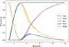 |
Fig. 1. He I (red), He II (blue), He III (yellow) fractions for late reionization (continuous curves) and early reionization (dashed curves) as a function of redshift. It is noteworthy that fHeI = 0 consistently for the Late model, whereas in the Early model, the first and second ionization of helium occur simultaneously. |
2.2. Brightness temperature
The differential brightness temperature δTb of the 3.46 cm hyperfine transition of He II with respect to the cosmic microwave background (CMB) is given by
![Mathematical equation: $$ \begin{aligned} \delta T_b(z,\mathbf r ) = \dfrac{T_S(z,\mathbf r ) - T_\mathrm{CMB} (z)}{1+z}\left[1-e^{-\tau (z,\mathbf r )}\right], \end{aligned} $$](/articles/aa/full_html/2026/03/aa58216-25/aa58216-25-eq1.gif) (1)
(1)
where TS(z, r) is the spin temperature associated to the spin-flip of the electron in the He II atoms, at redshift z and position r, TCMB(z) the CMB temperature and τ(z, r) the helium optical depth. In the optically thin regime τ ≪ 1, this corresponds to (Furlanetto et al. 2006):
![Mathematical equation: $$ \begin{aligned} \delta T_b(z,\mathbf r )&\simeq \dfrac{T_S(z,\mathbf r ) - T_\mathrm{CMB} (z)}{1+z}\tau (z,\mathbf r ) \nonumber \\&\simeq 0.58\, f_\mathrm{HeII} (z,\mathbf r )\Delta _b (1+z)^2 \frac{H_0}{H(z)} \\&\quad \times \left[ 1 - \dfrac{T_\mathrm{CMB} (z)}{T_S(z,\mathbf r )}\right] \left[ \dfrac{H(z)/(1+z)}{\mathrm{d} v_\parallel / \mathrm{d} r_\parallel } \right] \,\upmu \mathrm{K} ,\nonumber \end{aligned} $$](/articles/aa/full_html/2026/03/aa58216-25/aa58216-25-eq2.gif) (2)
(2)
where fHeII is the local fraction of He II, Δb (=ρb/ρc) the matter overdensity and dv∥/dr∥ as the velocity gradient along the line-of-sight, including both the Hubble expansion and the peculiar velocity. In this work we assume that  .
.
2.3. Spin temperature
Three processes contribute to the spin temperature: i) the coupling to the CMB temperature, ii) the collisional (de-)excitation, iii) the absorption and re-emission of Lyman-series photons (Field 1958; Takeuchi et al. 2014). As a first approximation, the spin temperature is given by the equilibrium of these processes,
 (3)
(3)
where Tα the temperature of the Ly-α radiation, TK is the gas kinetic temperature, closely coupled with Tα by recoil during repeated scattering and with the gas temperature (i.e. Tg ≃ TK ≃ Tα), yc is the coupling coefficient related to atomic collisions and yα is the coupling coefficient due to the scattering of Ly-α photons.
Both coupling coefficients are proportional to the rest-frequency of the emission line and to the inverse of the spontaneous decay rate, boosting the signal with respect to the 21 cm line from neutral hydrogen. However, both the collisional de-excitation rate and the de-excitation driven by He II Lyman-α scattering are extremely small for the 3He+ hyperfine transition. The dominant limitation is the very low abundance of 3He (n3He/nH ∼ 10−5), which strongly suppresses both collisional and radiative coupling irrespective of the detailed cross-sections. In addition, the relevant spin–exchange cross-sections and the background flux at the He II Lyman-α wavelength are themselves small, further reducing the efficiency of these processes. As a result, efficient coupling occurs only in the densest and coolest regions of the IGM, while the diffuse IGM remains only weakly coupled.
Contrary to K10 and B25, where the spin temperature is approximated to the gas temperature4, we compute the spin temperature following Equation (3) (Takeuchi et al. 2014), i.e. accounting for the coupling with both atomic collisions and scattering of Ly-α photons. We assume the model of UV/X-ray background from Haardt & Madau (2012) for the Ly-α flux as a function of redshift.
Figures 2a and 2b show the spin temperature for different redshifts for each model. It is worth noting that TS ≥ TCMB at all redshifts in the Late model, but not for the Early one, where a mixture of neutral, single-ionized and double-ionized helium is always present. Moreover, the spin temperature distribution considering three overdensities, Δb = 1, 10, 50, in red, orange and blue, in shown. As expected, in both models the spin temperature is higher for larger overdensities, making δTb an optimal tracer of the underlying matter distribution.
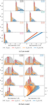 |
Fig. 2. Spin temperature distribution for both models at various redshifts. For each snapshot, the panels show the number of simulation voxels whose spin temperature falls within a given bin, N, as a function of the spin temperature. The spin temperature values corresponding to three overdensities, Δb = 1, 10, 50, are highlighted in red, orange and blue. The bottom-right panels display the evolution of the mean spin temperature with redshift together with its standard deviation. |
Outside the high-density regions discussed above, the spin temperature remains strongly coupled to the CMB. Therefore, the CMB temperature cannot generally be neglected relative to the spin temperature, resulting in (1 − TCMB/TS) ≉ 1 in Eq. (2).
Bagla & Loeb (2009) noted that Lyα coupling for the 3He II hyperfine transition may be affected by additional radiative-transfer subtleties, due to the proximity of the 3He II and 4He II Lyα resonances and potential contamination from nearby metal lines (e.g., O III). We do not model these line-overlap effects explicitly, and instead compute TS using an effective Lyα background (Madau & Haardt 2015), following Takeuchi et al. (2014). We expect this approximation to be adequate for our purposes, since the 3.46 cm signal in our simulations is dominated by overdense regions where collisional coupling is efficient.
Unresolved small–scale density structure below the spatial resolution of our simulations could, in principle, enhance the 3.46 cm signal. In the fully coupled regime the differential brightness temperature scales approximately linearly with overdensity, δTb ∝ Δb, so sub–grid clumping does not alter the mean signal. A possible boost could arise if the factor (1 − TCMB/TS) exhibited a strong density dependence, since in that case ⟨δTb(Δb)⟩ ≠ δTb(⟨Δb⟩), analogous to the clumping corrections for processes that scale as Δb2. However, in the redshift range relevant for this work (prior to the completion of helium reionization), the dependence of TS on overdensity is only mildly super–linear (Takeuchi et al. 2014), and becomes significant only at lower redshifts where the He II fraction is already negligible. Therefore, sub–megaparsec clumping is expected to induce at most a very small enhancement of the He II hyperfine signal.
3. Power spectrum
Denoting by δTb(q) the Fourier transform of the differential brightness temperature, where q are wavevectors with Cartesian components integer multiples of the fundamental frequency kF = 2π/L (for this work, kF = 0.0628 h Mpc−1), the estimator of its power spectrum is
 (4)
(4)
Nq is the number of q vectors in the k-bin of width δk and the sum is run over the q vectors such as k − δk/2 ≤ |q|< k + δk/2.
The mean power spectrum of the He Ii signal, along with the standard deviation over the set of simulations, is shown for the Late model in Figure 3 and for the Early model in Figure 4, together with the corresponding brightness temperature field from a representative simulation run. A clear distinction emerges when comparing the signal strengths of the two models at the same redshift. This difference arises from the distinct reionization timelines adopted in the Late and Early models. These results underscore how the timing of helium reionization strongly influences the amplitude and evolution of the He II signal as reflected in the power spectrum.
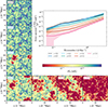 |
Fig. 3. Maps of the brightness temperature for the Late model at various redshifts, accompanied by the corresponding power spectra. The continuous curves represent the mean power spectra in the simulations, while the shaded regions show the 1σ scatter around the mean. |
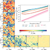 |
Fig. 4. Same as Fig. 3, but assuming the early reionization scenario. To enhance the morphology of the signal, a different color scale for the brightness temperature is used. |
As reionization progresses, the bubbles expand, merge, and fill the intergalactic medium. This expansion creates distinct patterns in the power spectrum on large scales. The growing bubbles generate regions with enhanced He II fraction surrounded by regions with lower He II fraction, introducing fluctuations in the signal and changing the topology of the He II field, transitioning from isolated and small bubbles to interconnected structures. In the Late model, where helium reionization occurs later and helium has already been ionized once, the He III bubbles dominate and contain negligible He II fraction inside them. The signal is produced outside the bubbles. In the Early model, helium is neutral at the beginning of the simulation, resulting in the formation of bubbles containing both He II and He III. Inside the bubbles, He III dominates, while the He II fraction is concentrated at the boundaries. Thus, the He II signal mainly arises from the edges of such bubbles.
The brightness temperature of the 3.46 cm signal from Equation (2) is determined by both the He II fraction and the underlying matter density distribution. As such, we expected the power spectrum of the signal to reflect contributions from both components (Figure 5 shows a comparison between the He II power spectrum and the rescaled matter power spectrum at the same redshift). However, because the spin temperature plays a dominant role in shaping the brightness temperature (effectively suppressing the signal in low-density regions) the resulting 3.46 cm power spectrum more closely resembles the shape of the matter power spectrum than initially anticipated. While the amplitude differs due to fixed scaling constants, the imprint of ionized bubble structures is less apparent than expected.
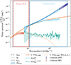 |
Fig. 5. Analysis of the power spectrum of the 3.46 cm line signal at redshift z = 4 for the late reionization scenario. Shown are the measured power spectrum from the simulations (solid blue line), the spectrum after accounting for the finite pixel size (dashed light-blue line), and the spectrum after Gaussian smoothing due to the angular resolution (dash-dotted green line). The rescaled matter power spectrum is displayed both in its raw form (solid orange line) and after smoothing (dotted orange line). Shaded regions indicate the 1σ scatter across the different simulation runs. The k-range accessible to SKA1-MID in single-dish (interferometic) mode is highlighted in red (blue). Vertical reference scales denote the wavenumbers corresponding to the telescope’s maximum angular resolution (kB, dotted black line), its field of view (kFOV, dash-dotted black line), and its pointing area (karea, dashed black line). The Gaussian smoothing applied corresponds to the angular resolution of SKA1-MID at z = 4. |
Some evidence of deviation from this behavior emerges in the Late model when comparing the power spectra at redshifts z = 5 and z = 4.5. At z = 5, the 3.46 cm power spectrum closely follows that of the matter distribution. At z = 4.5, however, we observe a modest enhancement at high k-modes (corresponding to small scales), likely reflecting the contribution from He II ionized bubbles. At low k-modes (large scales), the power spectrum remains consistent with the matter distribution, suggesting that the bubble signal has only a limited impact on the overall structure at those scales.
Our forecasts yield power-spectrum amplitudes that are roughly two orders of magnitude lower than those reported by B25, who obtained Δ(k = 0.1 h Mpc−1)≃10−1 μK for the 3He+ hyperfine transition at z ≃ 4. At the same scale and redshift, we find Δ(k = 0.1 h Mpc−1)≃10−3 μK (corresponding to Δ2 ≃ 10−6 μK2). This discrepancy originates from our self–consistent treatment of the spin–temperature coupling in the He II hyperfine signal: unlike B25, who effectively assume TS ≫ TCMB, we compute TS from collisional and Lyα coupling, which keeps it only slightly above the CMB temperature over most of the IGM (see Sect. 2.3). As a result, the factor (1−TCMB/TS) remains well below unity (Fig. 2), suppressing the amplitude of δTb and hence the power spectrum by roughly two orders of magnitude. A qualitative interpretation of the He II power spectrum in terms of clustering and shot–noise regimes is provided in Section 4.7.
4. Forecast for upcoming surveys
We forecast helium reionization detectability for three radio surveys, operating in single-dish or interferometric configurations. The main technical features of the surveys are listed in Table 1.
Technical parameters of the radio surveys considered in this work for the purposes of He II detection.
The first one we consider is the Square Kilometre Array Phase 1 MID (SKA-1 MID), a precursor to the full Square Kilometre Array (SKA) project. It will consist of an array of mid-frequency radio telescopes, and it will have a large collecting area and high sensitivity, making it well suited for studying the epoch of reionization and other cosmological open questions (Square Kilometre Array Cosmology Science Working Group 2020).
The second radio survey we take into account is the Deep Synoptic Array 2000 (DSA-2000), a proposed radio survey telescope with 2000 × 5 m dishes. It aims to image the entire sky repeatedly over sixteen epochs, detecting over one billion radio sources and operating as a dedicated survey telescope (Hallinan et al. 2019).
Finally, the Packed Ultra-wideband Mapping Array (PUMA) is a proposed radio telescope designed for 21 cm intensity mapping in the post-reionization era as well as other science goals, such as fast radio bursts, pulsar monitoring, and multi-messenger observations of transients. In the first phase, it consists of 5000 × 6 m antennas (Slosar et al. 2019).
The redshift range target by these instrument, when looking at the 3.46 cm hyperfine transition, overlap with helium reionization completely for SKA-1 MID and DSA-2000 but only partially for PUMA. However, PUMA is the most advanced of the instruments considered, owing to its very large number of antennas and dense configuration, which make it particularly interesting for studies of helium reionization. For this reason, as a proof of concept, we consider here a PUMA-like survey, i.e. a survey technically identical to PUMA but with a frequency bandwidth compatible with helium reionization.
We take into consideration the various systematic effects that arise during observations of the 3.46 cm hyperfine transition brightness temperature. As we are evaluating the surveys’ performances in both single-dish (SD) and interferometric (INT) configurations, we describe here the systematic effects in both cases. Regarding the single-dish configuration, we account for various factors including the frequency bandwidth selection (Section 4.1), the angular resolution of the telescope (Section 4.2), the foreground removal procedure (Section 4.3), and the thermal noise associated with the instrument (Section 4.4). The impact of these effects on the measured power spectrum are shown in Figure 5, where the measured power spectrum (in the Late scenario at redshift z = 4) is reported for reference as blue continuous line. The thermal noise of the detector in an interferometric configuration differs from the one considered in a single-dish setup and it is described in Section 4.5.
4.1. Frequency bandwidth and pixel size
When performing observations, the total receiver bandwidth is partitioned into frequency channels. Narrower channels offer better spectral resolution but lower sensitivity, while wider channels sacrifice spectral resolution for improved signal-to-noise ratio and sensitivity to large-scale structures. Selecting the optimal channel bandwidth involves balancing these factors based on the scientific goals and instrumental constraints of the tomography. The relation between redshift and comoving distance allows us to determine the channel bandwidth Δν at a specific redshift z corresponding to a given radial separation in comoving distance Δχ, as
 (5)
(5)
Accounting for the Cartesian grid size of the simulations, we set Δχ = L/Ngrid = 0.78 h−1 Mpc (≃0.5 MHz at z = 4), i.e. the smallest comoving distance accessible in the direction parallel to the line-of-sight within the simulation (verified to be larger than the frequency resolution of each instrument).
4.2. Angular resolution
To account for the finite angular resolution of the instrument, when operating in a single-dish setup, we incorporate a two-dimensional Gaussian filter in the observational plane, which we convolve with the simulated data cube in Fourier space. The full width at half maximum (FWHM) of the Gaussian beam is given by5
 (6)
(6)
where D is the diameter of the telescope antenna, reported in Table 1 for each telescope. This corresponds to an isotropic Gaussian smoothing with standard deviation
 (7)
(7)
where da is the angular-diameter distance to redshift z in the background (in a flat universe, (1 + z) da = χ). It follows that θFWHM ≈ 0.79 deg and Σ ≈ 29.3 h−1 Mpc at z = 4 for e.g., SKA-1 MID.
In the direction perpendicular to the line-of-sight, the solid angle covered by each pixel is Ωpix ≃ θpix2. To ensure proper sampling of the map and satisfy the Nyquist-Shannon theorem, the angular size of each pixel should be smaller than θFWHM. In practical terms, θpix is typically chosen to be between θFWHM/7 and θFWHM/3 (Marr et al. 2015). This range ensures that the map is adequately sampled, capturing the necessary level of detail without introducing significant aliasing effects.
The effects on the measured power spectrum when considering the proper pixel size and the telescope beam are shown respectively as the dashed light-blue line and the dash-dotted green line in Figure 5. The apparent roll-off at high k arises from the effective Nyquist limit imposed by the chosen pixel size, which ensures adequate sampling but slightly suppresses power near the resolution limit.
4.3. Foregrounds removal
Distinguishing the contributions of Galactic and extragalactic sources from the He II or H I signal poses a significant challenge in contemporary radio astronomy. Foreground emissions typically exhibit a smooth frequency dependence, unlike the fluctuating 3.46 cm signal, which demonstrates poor correlation in frequency space. Additionally, the high rest-frequency of the helium hyperfine transition helps mitigate contamination from synchrotron radiation and the terrestrial ionosphere (Takeuchi et al. 2014). These factors enable the development of pipelines specifically designed to extract the He II signal from observations. We do not simulate the foregrounds contribution to the signal (only for then to remove it using such techniques) but we provisionally assume that the foreground cleaning technique removes only the mean of the signal (the k = 0 mode of the Fourier transformed signal) while it leaves untouched the fluctuations around it.
While the dominant foregrounds in 1.42 GHz LIM are spectrally smooth (e.g., synchrotron and free-free emission), line-intensity mapping at 8.67 GHz may be affected by spectral confusion from line interlopers. In particular, low redshift HI emission can overlap in observed frequency with the He II 3.46 cm line at z > 5, while molecular lines (e.g., OH) and hydrogen recombination lines may introduce additional fluctuations. These interlopers are not necessarily spectrally smooth and could therefore survive foreground-cleaning techniques based on low-rank subtraction or high-pass filtering. While some of these contaminants (e.g., low-z HI) may be identifiable due to their brightness and clustering properties, their removal is non-trivial and depends on both the instrument sensitivity and survey design. In addition, man–made radio-frequency interference (RFI), including satellite broadcasting and communication signals in the UHF band (∼0.3–3 GHz), may further contaminate observations of the He II line at z ≃ 4–10.
A comprehensive treatment of line interlopers (e.g., via cross-correlation techniques or blind line separation algorithms) is beyond the scope of this work but will be crucial for future detection efforts. For the purposes of this forecast, we conservatively assume HeII dominates the line signal, and defer detailed modeling of line confusion to future work.
4.4. Single-dish thermal noise
The observed signal is contaminated by the radio telescope thermal noise, which is Gaussian to first approximation. The rms noise fluctuation depends on the system temperature, Tsys; the integration time per pointing, tpix; and the channel bandwidth, as
 (8)
(8)
For SKA-1 MID, Tsys is given by the sum of several components and strongly depends on frequency (Square Kilometre Array Cosmology Science Working Group 2020), as
 (9)
(9)
where Tspl ≈ 3 K and TCMB ≈ 2.73 K denote the spillover and the cosmic-microwave-background contributions, respectively. The Galaxy contribution can be modeled as
 (10)
(10)
and the receiver-noise temperature as
 (11)
(11)
This gives very large values of the system temperature for low redshifts (e.g., Tsys(z = 3)≈81 K), a minimum around z ≈ 8.5 (Tsys(z = 8.5)≈24 K) and a gentle rise for higher redshifts (e.g., Tsys(z = 11)≈26 K). It follows that, for fixed values of tpix and Δν, the level of thermal noise is minimized for intermediate redshifts. For DSA-2000 and PUMA, the system temperature is approximated to 25 K (Hallinan et al. 2019; Slosar et al. 2019) independently of frequency.
The integration time, tobs, needed to map a portion of the sky over the solid angle Ωsurv is given by
 (12)
(12)
where Ndish is the number of antennas (see Table 1), each with Nbeam (=1 for the surveys we considered) feedhorns.
The analytical expression for the variance of the power spectrum due to the thermal noise, defined in Equation (8) is given by
 (13)
(13)
where Asurv is the area covered by the survey in physical units (while we denote as Ωsurv the corresponding solid angle) and lpix is the physical length of the channel width (here chosen to be equal to Δχ as defined in Section 4.1).
4.5. Interferometer thermal noise
In an interferometric setup, two antennas separated by a baseline of length d measure a visibility V(u, ν), where u = |u| = d/λ denotes the baseline projected onto the uv-plane. The resolution in uv-space is governed by the instrument’s field of view (FOV), which, for an array of dishes, corresponds to the beam solid angle of an individual dish. This implies a typical resolution of δu, δv ∼ 1/FOV ∼ Ae/λ2, where Ae is the effective area of a single dish (Ae ≃ π(D/2)2). Visibilities that are separated by more than this scale in uv-space can be treated as statistically uncorrelated. For scales smaller than Ae/λ2, one can average all visibilities within each resolution element of area δu, δv. This averaging reduces the noise by the number of visibilities per element, while the sky signal remains effectively unchanged (provided the uv sampling is sufficiently fine). The noise in each uv resolution element is then
![Mathematical equation: $$ \begin{aligned} \sigma _\mathrm{int} (\mathbf u ,\nu ) = \dfrac{T_\mathrm{sys} (z)}{\sqrt{t_\mathrm{obs} \Delta \nu }} \dfrac{\left[\lambda _{\mathrm {He}{\small { {\text{ II}}}}}\mathrm {(1+z)}\right]^2}{A_e} \dfrac{1}{\sqrt{N_b(\mathbf u )}}, \end{aligned} $$](/articles/aa/full_html/2026/03/aa58216-25/aa58216-25-eq15.gif) (14)
(14)
where Nb(u) (=Nb(u) due to symmetric arguments) is the number density of baselines. If we assume that Nb(u) is constant on the uv plane between some umin = D/(λHe II (1+z)) and umax =B/(λHe II (1+z)), where B is the core baseline of the survey (i.e. where the largest fraction of antenna is concentrated), we can write
 (15)
(15)
Note that this is not the same as assuming an uniform distribution of antennas.
Following Bull et al. (2015) and references within (e.g., McQuinn et al. 2006; Geil et al. 2011; Villaescusa-Navarro et al. 2014), the power spectrum of the detector noise for interferometric observations, analog to the one defined in Equation (13), reads
![Mathematical equation: $$ \begin{aligned} N_\mathrm{int} (z) \simeq 7 \left(\dfrac{B}{D} \right)^2 \dfrac{T^2_\mathrm{sys} (z)}{N^2_\mathrm{ dish} } \dfrac{1}{\Delta \nu } \dfrac{A_\mathrm{FOV} }{t_\mathrm{obs} } \left[\dfrac{\Delta \nu }{\nu _\mathrm{HeII} } \dfrac{c(1+z)^2}{H(z)} \right], \end{aligned} $$](/articles/aa/full_html/2026/03/aa58216-25/aa58216-25-eq17.gif) (16)
(16)
where AFOV ∼ θFWHM2 is the survey area (that corresponds to the field of view for an interferometer). The squared-brackets factor corresponds to the channel width in physical units.
4.6. k-modes selection
It is important to carefully select the relevant scales when designing a radio survey, whether operated in single-dish mode or as an interferometer. In the former case, the accessible scales are limited by the angular resolution of each antenna (kFOV) and by the total area covered in each pointing (karea). In contrast, interferometers–thanks to their higher angular resolution–can access larger k-modes, constrained by the instrument’s field of view (kFOV) and by the maximum baseline length (kB). These characteristic scales depend on the specific instrument and the redshift under consideration, and are defined as6:
 (17)
(17)
 (18)
(18)
 (19)
(19)
For example for SKA-1 MID, we find kB(z = 4) = 7.29 h Mpc−1 and kFOV(z = 4) = 0.11 h Mpc−1. In this work, we assume an area per pointing7 of Ωarea = 4 × 10⁻³ sr (=13deg2), corresponding to karea(z = 4) = 0.02 h Mpc−1. These scales are shown in Figure 5 as black vertical lines and denote the range of sensitivity for the two configurations. The power spectrum measured from the simulations considered in this work is limited by the size of the box (kF = 0.0628 h Mpc−1) and by its resolution, and it does not cover the all range of wavelengths needed to evaluate both configurations (karea ≤ k ≤ kFOV for single-dish mode and kFOV ≤ k ≤ kB for an interferometer). Moreover, while in principle kmax = 2π/(L/Ngrid) = 2π/(100 h−1 Mpc/128) = 8.04 h Mpc−1, resolution effects are noticed already from k ∼ 4 h Mpc−1 (for this reason the power spectrum is measured and presented in Figure 5 up until k ≃ 3 h Mpc−1). How to extend the power spectrum measured from simulations to the wavelengths of interests for this work is the subject of the next sections.
Equations (17)–(19) specify the transverse wavenumber limits k⊥ set by the baselines, dish size, and survey area. The radial modes, k∥, are instead fixed by the channel width and total bandwidth. For the frequency resolutions considered here, the sampling in k∥ is much denser than in k⊥, so that k∥ can be treated as effectively continuous. Consequently, the transverse limits k⊥, min and k⊥, max can be used as the effective bounds on the total wavenumber.
It is plausible that extending the integration over a broader range of scales, particularly at low-k for single-dish and high-k for interferometers, would marginally increase SNR, especially for instruments such as DSA-2000 and PUMA, whose configurations offer access to both regimes. Future forecasts should incorporate full instrument sensitivity curves overlaid on the simulated power spectrum to optimize k-space coverage.
4.6.1. Single-dish configuration
As mentioned already in Section 3, the 3.46 cm signal is affected not only by the ionization state of helium but also by the underlying dark matter density. This last contribution leads for small k-modes, while the He III bubbles seems boosting the signal at higher k-modes. In the attempt of disentangle the two contribution, we compute the linear matter power spectrum with CAMB (Lewis et al. 2000) and we compare it with the power spectrum of the 3.46 cm signal after a properly rescale (by a factor C, depending on the redshift considered). The matching of the two power spectra on large scales (k ≳ 0.06 h Mpc−1) is shown in Figure 5 as the orange continuous line. In order to gain access to scales larger than the one available with our simulations, we extend the brightness temperature power spectrum on the left-hand side, i.e. for scales 0.015 h Mpc−1 < k < 0.06 h Mpc−1. The dotted orange line in Figure 5 exhibits the convolution between the scaled theoretical power spectrum and the window function implementing the smoothing in the directions parallel and perpendicular to the line-of-sight, P(k)CAMB ⋅ W(k, Δχ, Σ). The window function reads (Li et al. 2016)
 (20)
(20)
where μ = cos θ with θ the spherical polar angle in k-space. We display in Figure 5 as red points the selected k-values extrapolated from the smoothed rescaled matter power spectrum.
4.6.2. Interferometer configuration
The largest k-mode accessible from simulations is set by their resolution, but it is limited to kcut − off ≃ 3 h Mpc−1 (corresponding to a scale of ∼2 h−1 Mpc) to avoid resolution effects in the computation of the power spectrum. We notice, from the analysis of the power spectrum, that these scales are well traced by the matter power spectrum when accounting for a small boost due to the He III bubbles. We extrapolate the k-modes between kcut − off and kB by fitting a power law to the power spectrum at large k-modes, and sampling using the same δk. These k-values are shown as dark blue points in Figure 5.
4.7. Clustering and shot-noise regimes of the He II power spectrum
The physical interpretation of the 3.46 cm power spectrum depends on the spatial scales probed. On large scales (low k), fluctuations predominantly trace the clustering of He II regions around AGN and broadly follow the underlying matter density field. On small scales (high k), the signal becomes dominated by the discreteness of these ionized structures and by the strong concentration of emission within overdense gas, in qualitative analogy with the shot-noise regime familiar from mm-wave and 21 cm line-intensity mapping. This scale dependence has direct implications for observations: interferometric arrays are intrinsically more sensitive to the small-scale, shot-noise-dominated component of the signal, while single-dish surveys preferentially probe the large-scale clustering power.
The transition scale depends on the spatial distribution and duty cycle of AGN. While this behavior is well known in mm-wave and 21 cm LIM (e.g., Breysse et al. 2017; Uzgil et al. 2019), it has not been explicitly studied for the HeII hyperfine transition. Our simulations suggest that the HeII signal in overdense regions leads to enhanced power at small scales, consistent with a hybrid clustering–shot-noise regime.
5. Signal-to-noise ratio
In our pursuit of assessing the detectability of the signal within current radio astronomy surveys, it is helpful to define the signal-to-noise ratio for the power spectrum as
![Mathematical equation: $$ \begin{aligned} \mathrm{S/N} ^2(k) = \dfrac{P^2(k)}{\sigma _P^2(k)} = N_q \dfrac{P^2(k)}{\left[P(k) + N \right]^2}, \end{aligned} $$](/articles/aa/full_html/2026/03/aa58216-25/aa58216-25-eq22.gif) (21)
(21)
where N denotes the power spectrum of the detector noise for either single-dish (NSD, defined in Equation (13)) or interferometric configurations (Nint, defined in Equation (16)), and the number of modes within the k-bin of width δk is
 (22)
(22)
where Vsurv = Asurvls is the volume of the survey given by the observed area perpendicular to the line-of-sight Asurv and the comoving distance in the direction parallel to the line of sight, ls.
The standard deviation on the power spectrum, as defined in Equation (21), accounts for the contribution of the number of independent modes within the i-th bin (the higher it is, the smaller is the error on the power spectrum) and of the white noise introduced by the instrument. As we are interested in quantifying the required integration time to detect the He II signal, we expressed the S/N as a function on tobs by combining Equations (12), (13), (21) and (22) for a single-dish configuration,
![Mathematical equation: $$ \begin{aligned} \mathrm{S/N} _\mathrm{SD} ^2 (k) = \dfrac{k^2 \delta k}{(2\pi )^2} A_\mathrm{surv} l_\mathrm{s} \left[1 + \dfrac{1}{P(k)} \dfrac{T_\mathrm{sys} ^2 A_\mathrm{surv} l_\mathrm{pix} }{t_\mathrm{obs} N_\mathrm{dish} N_\mathrm{beam} \Delta \nu } \right]^{-2}. \end{aligned} $$](/articles/aa/full_html/2026/03/aa58216-25/aa58216-25-eq24.gif) (23)
(23)
Note that for a given instrument, at a given redshift, at a given scale, Equation (23) reads S/N ∝ ls1/2Asurv−1/2tobs. Therefore, an optimal S/N is achieved when observing smaller areas but wider redshift ranges. For an interferometer setup, Equation (23) reads
![Mathematical equation: $$ \begin{aligned} \mathrm{S/N} _\mathrm{int} ^2 (k)&= \dfrac{k^2 \delta k}{(2\pi )^2} A_\mathrm{surv} l_\mathrm{s} \nonumber \\&\quad \times \left[1 + \dfrac{1}{P(k)} 7\left(\dfrac{B}{D}\right)^2\dfrac{T_\mathrm{sys} ^2 A_\mathrm{FOV} \lambda _\mathrm{HeII} }{t_\mathrm{obs} N_\mathrm{dish} N_\mathrm{beam} } \dfrac{(1+z)^2}{H(z)} \right]^{-2}. \end{aligned} $$](/articles/aa/full_html/2026/03/aa58216-25/aa58216-25-eq25.gif) (24)
(24)
To improve detection capabilities, it is advantageous to consider the integrated signal-to-noise ratio, denoted as S/Nt, obtained by combining the contributions from all scales, defined as
 (25)
(25)
Since the power spectrum varies with redshift, we utilize the mean power spectrum within the specified redshift range (3.5 ≤ z ≤ 5 for the Late model, 6 ≤ z ≤ 9 for the Early model) for our following analysis. We have presented in Section 4.6 and in Figure 5 the k values used in the calculation of S/Nt (it is worth noting that the same procedure is applied to other redshifts). These values include both those derived from the simulation boxes and those obtained from the scaled matter power spectrum. The relationship between the integration time, tobs, and the integrated signal-to-noise ratio, S/Nt, is presented in Figures 6 and 7 for single-dish observations, and in Figure 8 for interferometric observations.
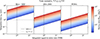 |
Fig. 6. Relation between the integration time (tobs) and the integrated signal-to-noise ratio (S/Nt) for the redshift range 3.5 ≤ z ≤ 5 for single-dish observations. Different colors represent different survey areas, Ωsurv, while the dotted black line shows a reference integration time of 1 year, and the dashed back lack line shows a reference S/Nt of 1. Each panel corresponds to a unique survey. |
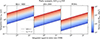 |
Fig. 7. Same as Fig. 6, but for the redshift range 6 ≤ z ≤ 9 and assuming an early reionization scenario. |
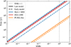 |
Fig. 8. Relation between the integration time and the integrated signal-to-noise ratio (S/Nt) for interferometric observations. Forecasts are shown for the three radio surveys considered, SKA-1 MID (blue), DSA-2000 (red) and PUMA-like (orange), and for the two reionization models studied in this work, Late (continuous lines) and Early (dashed lines) scenarios. The dotted black line marks a S/Nt of 1. |
For single-dish setups, we show results for a fixed line-of-sight depth, defined by the redshift ranges 3.5 ≤ z ≤ 5 (Late model) and 6 ≤ z ≤ 9 (Early model), and various survey areas Ωsurv across the three instruments considered. Optimal performance is obtained when observing a relatively compact region of the sky over an extended frequency range. Larger survey areas require significantly longer integration times to reach the same S/Nt, since the time per pixel decreases when spreading the observing time over a wider area. Among the three surveys, a PUMA-like configuration, thanks to its large number of antennas and intermediate dish size, provides the highest sensitivity. While SKA-1 MID and DSA-2000 would require prohibitively long observations to reach S/Nt ∼ 1, a PUMA-like survey in single-dish mode could achieve a marginal detection of the 3.46 cm signal (S/Nt of approximately a few) within ≲1000 h, in both reionization scenarios. Next-generation instruments may be able to access the He II hyperfine signal for the first time.
For interferometric observations all considered instruments require prohibitively long integration times, though the PUMA-like survey again performs best for both the Early and Late models. Compared to single-dish mode, interferometry is more sensitive to small-scale fluctuations where the He Ii signal peaks, but it also requires longer observations to reach a comparable S/Nt.
The underlying difficulty lies in the intrinsic faintness of the 3.46 cm signal. Because the spin temperature in low-density regions is only weakly coupled to the kinetic temperature, the differential brightness temperature is suppressed across much of the intergalactic medium. As a result, the signal is mostly generated in overdense regions, which coincide with the scales where instrumental noise and resolution limits are most restrictive.
Despite the low S/Nt, our simulations show that the Early and Late reionization models produce distinguishable power spectra. In the Early model, the presence of high-redshift quasars leads to an elevated He II fraction and a stronger signal at z ≳ 5, with a relatively flat power spectrum at small scales. In the Late model, the signal builds up more slowly and peaks at z ∼ 4, with a steeper shape and greater power at intermediate scales. These differences, though apparent in simulation, are effectively unobservable with current instrument sensitivities.
6. Summary and conclusion
In this work, we assessed the detectability of the 3.46 cm hyperfine transition of singly-ionized helium with upcoming and proposed radio surveys, using hydrodynamical simulations post-processed with radiative transfer to model early and late helium reionization scenarios. We computed the corresponding He II power spectra and evaluated the performance of SKA-1 MID, DSA-2000, and a PUMA-like array in both single–dish and interferometric observing modes.
Our results show that the intrinsic faintness of the 3.46 cm signal (driven also by weak spin–temperature coupling in most of the IGM) suppresses the brightness temperature and limits detectability for current surveys. Although the Early and Late models produce distinct power spectra in simulation, the predicted amplitudes are well below the thermal-noise levels of SKA-1 MID and DSA-2000, both in single-dish and interferometric setups. A PUMA-like survey in a single-dish setup, however, could detect the 3.46 cm signal with a S/Nt of a few in ≲1000 h. Such a detection would constitute a first step toward accessing the 3.46 cm signal, and even distinguish between early and late helium-reionization scenarios, constraining the sources of helium reionization. Future progress will likely require improved sensitivity, denser baseline coverage, larger bandwidths, or complementary approaches such as global-signal measurements or cross-correlations with galaxy surveys. Likewise, alternative statistics sensitive to higher-order moments and to the global geometry and topology of the He II field may further help differentiate reionization models. We note, moreover, that LIM is not the only observational pathway to the 3.46 cm transition. Complementary technique, such as the He II 3.46 cm forest toward bright high-redshift quasars presented in B25 or cross-correlations with galaxy or QSO catalogs, may provide additional, more accessible routes to detecting this signal. Larger-volume simulations would also be beneficial to better capture the accessible k-range and reduce sample variance on large scales.
Acknowledgments
BS carried out part of this work while being part of the International Max Planck Research School in Astronomy and Astrophysics and the Bonn Cologne Graduate School. BS and CP gratefully acknowledge the Collaborative Research Center 1601 (SFB 1601 sub-project C6) funded by the Deutsche Forschungsgemeinschaft (DFG, German Research Foundation) – 500700252. BS and SEIB are supported by the Deutsche Forschungsgemeinschaft (DFG) under Emmy Noether grant number BO 5771/1-1. CP is grateful to SISSA, the University of Trieste, and IFPU, where part of this work was carried out, for hospitality and support. We thank Fabian Walter, Anna Pugno and Elena Marcuzzo for the useful comments and discussions.
References
- Bagla, J. S., & Loeb, A. 2009, MNRAS, submitted [arXiv:0905.1698] [Google Scholar]
- Balser, D. S., & Bania, T. M. 2018, AJ, 156, 280 [Google Scholar]
- Balser, D. S., Goss, W. M., Bania, T. M., & Rood, R. T. 2006, ApJ, 640, 360 [NASA ADS] [CrossRef] [Google Scholar]
- Bandura, K., Addison, G. E., Amiri, M., et al. 2014, SPIE Conf. Ser., 9145, 914522 [NASA ADS] [Google Scholar]
- Barkana, R., & Loeb, A. 2005, ApJ, 626, 1 [Google Scholar]
- Basu, A., Garaldi, E., & Ciardi, B. 2024, MNRAS, 532, 841 [Google Scholar]
- Basu, A., Ciardi, B., & Garaldi, E. 2025, arXiv e-prints [arXiv:2510.14059] [Google Scholar]
- Battye, R. A., Browne, I. W. A., Dickinson, C., et al. 2013, MNRAS, 434, 1239 [NASA ADS] [CrossRef] [Google Scholar]
- Becker, G. D., Bolton, J. S., Haehnelt, M. G., & Sargent, W. L. W. 2011, MNRAS, 410, 1096 [NASA ADS] [CrossRef] [Google Scholar]
- Breysse, P. C., Kovetz, E. D., Behroozi, P. S., Dai, L., & Kamionkowski, M. 2017, MNRAS, 467, 2996 [NASA ADS] [Google Scholar]
- Bull, P., Ferreira, P. G., Patel, P., & Santos, M. G. 2015, ApJ, 803, 21 [NASA ADS] [CrossRef] [Google Scholar]
- Cantalupo, S., & Porciani, C. 2011, MNRAS, 411, 1678 [Google Scholar]
- Chardin, J., Puchwein, E., & Haehnelt, M. G. 2017, MNRAS, 465, 3429 [NASA ADS] [CrossRef] [Google Scholar]
- Chen, T., Battye, R. A., Costa, A. A., Dickinson, C., & Harper, S. E. 2020, MNRAS, 491, 4254 [NASA ADS] [CrossRef] [Google Scholar]
- Compostella, M., Cantalupo, S., & Porciani, C. 2014, MNRAS, 445, 4186 [NASA ADS] [CrossRef] [Google Scholar]
- Croom, S. M., Smith, R. J., Boyle, B. J., et al. 2004, MNRAS, 349, 1397 [NASA ADS] [CrossRef] [Google Scholar]
- Field, G. B. 1958, Proc. IRE, 46, 240 [NASA ADS] [CrossRef] [Google Scholar]
- Fontanot, F., Cristiani, S., Grazian, A., et al. 2023, MNRAS, 520, 740 [Google Scholar]
- Furlanetto, S. R. 2006, MNRAS, 370, 1867 [Google Scholar]
- Furlanetto, S. R., & Oh, S. P. 2008, ApJ, 681, 1 [Google Scholar]
- Furlanetto, S. R., Oh, S. P., & Briggs, F. H. 2006, Phys. Rep., 433, 181 [Google Scholar]
- Gaikwad, P., Srianand, R., Haehnelt, M. G., & Choudhury, T. R. 2021, MNRAS, 506, 4389 [NASA ADS] [CrossRef] [Google Scholar]
- Garaldi, E., Compostella, M., & Porciani, C. 2019, MNRAS, 483, 5301 [NASA ADS] [CrossRef] [Google Scholar]
- Garzilli, A., Theuns, T., & Schaye, J. 2020, MNRAS, 492, 2193 [Google Scholar]
- Geil, P. M., Gaensler, B. M., & Wyithe, J. S. B. 2011, MNRAS, 418, 516 [Google Scholar]
- Giallongo, E., Grazian, A., Fiore, F., et al. 2015, A&A, 578, A83 [NASA ADS] [CrossRef] [EDP Sciences] [Google Scholar]
- Glikman, E., Djorgovski, S. G., Stern, D., et al. 2011, ApJ, 728, L26 [NASA ADS] [CrossRef] [Google Scholar]
- Grazian, A., Giallongo, E., Boutsia, K., et al. 2022, ApJ, 924, 62 [NASA ADS] [CrossRef] [Google Scholar]
- Haardt, F., & Madau, P. 2012, ApJ, 746, 125 [Google Scholar]
- Hall, P. J. 2005, The Square Kilometre Array: An Engineering Perspective [Google Scholar]
- Hallinan, G., Ravi, V., Weinreb, S., et al. 2019, BAAS, 51, 255 [NASA ADS] [Google Scholar]
- Harikane, Y., Ouchi, M., Oguri, M., et al. 2023, ApJS, 265, 5 [NASA ADS] [CrossRef] [Google Scholar]
- Jakobsen, P., Boksenberg, A., Deharveng, J. M., et al. 1994, Nature, 370, 35 [NASA ADS] [CrossRef] [Google Scholar]
- Jiang, L., McGreer, I. D., Fan, X., et al. 2016, ApJ, 833, 222 [Google Scholar]
- Khullar, S., Ma, Q., Busch, P., et al. 2020, MNRAS, 497, 572 [Google Scholar]
- Lewis, A., Challinor, A., & Lasenby, A. 2000, ApJ, 538, 473 [Google Scholar]
- Li, T. Y., Wechsler, R. H., Devaraj, K., & Church, S. E. 2016, ApJ, 817, 169 [NASA ADS] [CrossRef] [Google Scholar]
- Linder, E. V. 2020, Phys. Rev. D, 101, 103019 [NASA ADS] [CrossRef] [Google Scholar]
- Madau, P., & Haardt, F. 2015, ApJ, 813, L8 [Google Scholar]
- Madau, P., Giallongo, E., Grazian, A., & Haardt, F. 2024, ApJ, 971, 75 [NASA ADS] [CrossRef] [Google Scholar]
- Marr, J., Snell, R., & Kurtz, S. 2015, Fundamentals of Radio Astronomy: Observational Methods (CRC Press), Ser. Astron. Astrophys. [Google Scholar]
- McQuinn, M., & Switzer, E. R. 2009, Phys. Rev. D, 80, 063010 [Google Scholar]
- McQuinn, M., Zahn, O., Zaldarriaga, M., Hernquist, L., & Furlanetto, S. R. 2006, ApJ, 653, 815 [NASA ADS] [CrossRef] [Google Scholar]
- Newburgh, L. B., Bandura, K., Bucher, M. A., et al. 2016, SPIE Conf. Ser., 9906, 99065X [Google Scholar]
- Parsa, S., Dunlop, J. S., & McLure, R. J. 2018, MNRAS, 474, 2904 [Google Scholar]
- Ricci, C., Trakhtenbrot, B., Koss, M. J., et al. 2017, ApJS, 233, 17 [Google Scholar]
- Richards, G. T., Strauss, M. A., Fan, X., et al. 2006, AJ, 131, 2766 [Google Scholar]
- Rood, R. T., Wilson, T. L., & Steigman, G. 1979, ApJ, 227, L97 [Google Scholar]
- Rood, R. T., Bania, T. M., & Wilson, T. L. 1984, ApJ, 280, 629 [Google Scholar]
- Shull, J. M., France, K., Danforth, C. W., Smith, B., & Tumlinson, J. 2010, ApJ, 722, 1312 [NASA ADS] [CrossRef] [Google Scholar]
- Slosar, A., Ahmed, Z., Alonso, D., et al. 2019, BAAS, 51, 53 [Google Scholar]
- Spina, B., Porciani, C., & Schimd, C. 2021, MNRAS, 505, 3492 [CrossRef] [Google Scholar]
- Square Kilometre Array Cosmology Science Working Group (Bacon, D. J., et al.) 2020, PASA, 37, e007 [Google Scholar]
- Syphers, D., Anderson, S. F., Zheng, W., et al. 2011, ApJ, 726, 111 [Google Scholar]
- Takeuchi, Y., Zaroubi, S., & Sugiyama, N. 2014, MNRAS, 444, 2236 [Google Scholar]
- Teyssier, R. 2002, A&A, 385, 337 [CrossRef] [EDP Sciences] [Google Scholar]
- Theuns, T., Schaye, J., Zaroubi, S., et al. 2002, ApJ, 567, L103 [Google Scholar]
- Trott, C. M., & Wayth, R. B. 2024, ApJ, 960, 10 [Google Scholar]
- Uzgil, B. D., Carilli, C., Lidz, A., et al. 2019, ApJ, 887, 37 [Google Scholar]
- van Haarlem, M. P., Wise, M. W., Gunst, A. W., et al. 2013, A&A, 556, A2 [NASA ADS] [CrossRef] [EDP Sciences] [Google Scholar]
- Vasiliev, E. O., Sethi, S. K., & Shchekinov, Y. A. 2019, MNRAS, 490, 5057 [Google Scholar]
- Villaescusa-Navarro, F., Viel, M., Datta, K. K., & Choudhury, T. R. 2014, JCAP, 2014, 050 [Google Scholar]
- Walther, M., Oñorbe, J., Hennawi, J. F., & Lukić, Z. 2019, ApJ, 872, 13 [NASA ADS] [CrossRef] [Google Scholar]
- Worseck, G., Prochaska, J. X., Hennawi, J. F., & McQuinn, M. 2016, ApJ, 825, 144 [NASA ADS] [CrossRef] [Google Scholar]
- Worseck, G., Davies, F. B., Hennawi, J. F., & Prochaska, J. X. 2019, ApJ, 875, 111 [Google Scholar]
- Worseck, G., Khrykin, I. S., Hennawi, J. F., Prochaska, J. X., & Farina, E. P. 2021, MNRAS, 505, 5084 [NASA ADS] [CrossRef] [Google Scholar]
- Yang, G., Caputi, K. I., Papovich, C., et al. 2023, ApJ, 950, L5 [NASA ADS] [CrossRef] [Google Scholar]
The following cosmological parameters were adopted: matter density Ωm = 0.2726, baryon density Ωb = 0.0456, Hubble constant H0 = 100 h km s−1 Mpc−1 with h = 0.704, spectral index ns = 0.963, and linear rms fluctuation σ8 = 0.809 within spheres of radius 8 h−1 Mpc.
With cosmological parameters Ωm = 0.306, Ωb = 0.0483, H0 = 100 h km s−1 Mpc−1 with h = 0.679, ns = 0.958, and σ8 = 0.815.
K20 focused mainly on the temperature fluctuations around QSOs (i.e. in overdense regions, where TS ≫ TCMB).
Ideal illumination gives a coefficient of 1.02 (e.g., Hall 2005; Chen et al. 2020), while tapering and sidelobes can raise it to ∼1.4. We adopt 1.2 as a standard effective value (Spina et al. 2021).
Assuming a flat universe, for which (1 + z) da = χ.
The antenna of a radio survey operating in single-dish mode observes only a limited sky region per pointing. The total survey area, Asurv, can nevertheless be made arbitrarily large by combining multiple pointings over the full observing time.
All Tables
Technical parameters of the radio surveys considered in this work for the purposes of He II detection.
All Figures
|
Fig. 1. He I (red), He II (blue), He III (yellow) fractions for late reionization (continuous curves) and early reionization (dashed curves) as a function of redshift. It is noteworthy that fHeI = 0 consistently for the Late model, whereas in the Early model, the first and second ionization of helium occur simultaneously. |
| In the text | |
|
Fig. 2. Spin temperature distribution for both models at various redshifts. For each snapshot, the panels show the number of simulation voxels whose spin temperature falls within a given bin, N, as a function of the spin temperature. The spin temperature values corresponding to three overdensities, Δb = 1, 10, 50, are highlighted in red, orange and blue. The bottom-right panels display the evolution of the mean spin temperature with redshift together with its standard deviation. |
| In the text | |
|
Fig. 3. Maps of the brightness temperature for the Late model at various redshifts, accompanied by the corresponding power spectra. The continuous curves represent the mean power spectra in the simulations, while the shaded regions show the 1σ scatter around the mean. |
| In the text | |
|
Fig. 4. Same as Fig. 3, but assuming the early reionization scenario. To enhance the morphology of the signal, a different color scale for the brightness temperature is used. |
| In the text | |
|
Fig. 5. Analysis of the power spectrum of the 3.46 cm line signal at redshift z = 4 for the late reionization scenario. Shown are the measured power spectrum from the simulations (solid blue line), the spectrum after accounting for the finite pixel size (dashed light-blue line), and the spectrum after Gaussian smoothing due to the angular resolution (dash-dotted green line). The rescaled matter power spectrum is displayed both in its raw form (solid orange line) and after smoothing (dotted orange line). Shaded regions indicate the 1σ scatter across the different simulation runs. The k-range accessible to SKA1-MID in single-dish (interferometic) mode is highlighted in red (blue). Vertical reference scales denote the wavenumbers corresponding to the telescope’s maximum angular resolution (kB, dotted black line), its field of view (kFOV, dash-dotted black line), and its pointing area (karea, dashed black line). The Gaussian smoothing applied corresponds to the angular resolution of SKA1-MID at z = 4. |
| In the text | |
|
Fig. 6. Relation between the integration time (tobs) and the integrated signal-to-noise ratio (S/Nt) for the redshift range 3.5 ≤ z ≤ 5 for single-dish observations. Different colors represent different survey areas, Ωsurv, while the dotted black line shows a reference integration time of 1 year, and the dashed back lack line shows a reference S/Nt of 1. Each panel corresponds to a unique survey. |
| In the text | |
|
Fig. 7. Same as Fig. 6, but for the redshift range 6 ≤ z ≤ 9 and assuming an early reionization scenario. |
| In the text | |
|
Fig. 8. Relation between the integration time and the integrated signal-to-noise ratio (S/Nt) for interferometric observations. Forecasts are shown for the three radio surveys considered, SKA-1 MID (blue), DSA-2000 (red) and PUMA-like (orange), and for the two reionization models studied in this work, Late (continuous lines) and Early (dashed lines) scenarios. The dotted black line marks a S/Nt of 1. |
| In the text | |
Current usage metrics show cumulative count of Article Views (full-text article views including HTML views, PDF and ePub downloads, according to the available data) and Abstracts Views on Vision4Press platform.
Data correspond to usage on the plateform after 2015. The current usage metrics is available 48-96 hours after online publication and is updated daily on week days.
Initial download of the metrics may take a while.