| Issue |
A&A
Volume 708, April 2026
|
|
|---|---|---|
| Article Number | A107 | |
| Number of page(s) | 11 | |
| Section | Astrophysical processes | |
| DOI | https://doi.org/10.1051/0004-6361/202556087 | |
| Published online | 31 March 2026 | |
Long-term activity cycles in planetary M stars observed with SOPHIE
1
Instituto de Astronomía y Física del Espacio, CONICET–UBA, Buenos Aires, Argentina
2
Consejo Nacional de Investigaciones Científicas y Técnicas (CONICET), Godoy Cruz, 2290, CABA, CPC 1425FQB, Argentina
3
Instituto Tecnológico de Buenos Aires (ITBA), Iguazú 341 Buenos Aires, CABA, C1437, Argentina
4
Instituto de Ciencias Físicas (CONICET/ECyT-UNSAM), Campus Miguelete, 25 de Mayo y Francia, (1650), Buenos Aires, Argentina
5
Universidad Nacional de Córdoba – Observatorio Astronómico de Córdoba, Laprida 854, X5000BGR, Córdoba, Argentina
6
Aix Marseille Univ, CNRS, CNES, LAM, Marseille, France
7
Univ. Grenoble Alpes, CNRS, IPAG, 38000 Grenoble, France
★ Corresponding author: This email address is being protected from spambots. You need JavaScript enabled to view it.
Received:
24
June
2025
Accepted:
5
February
2026
Abstract
Context. M dwarfs are prime targets for exoplanet searches due to their low masses and radii, which enable the detection of small planets in their habitable zones (HZs). However, the magnetic activity of M dwarfs can introduce signals in radial velocity measurements that may be mistaken for planetary signatures, making the understanding of stellar activity cycles crucial for accurate planet detection and characterisation.
Aims. We aim to identify and characterise long-term magnetic activity cycles in M dwarfs using a homogeneous and extensive spectroscopic dataset in order to better understand their magnetic variability and its implications for exoplanet detection.
Methods. We analysed 13 years of high-resolution spectra obtained with the SOPHIE spectrograph for two early M dwarfs known to host exoplanets. We simultaneously monitored chromospheric activity using two indicators, the Hα index and the Mount Wilson S-index. Long-term trends were modelled using both sinusoidal and low-order polynomial fits to robustly identify stellar activity cycles. As a complement, we used TESS photometric data to assess the short-term variability of both targets.
Results. We detected long-term variability consistent with stellar magnetic cycles in both targets. For GJ 617A, we report a cycle of approximately 4.8 years, while for GJ 411, we find several characteristic timescales of variability of about 4.9 years. In addition, TESS photometric data reveal signs of short-term variability in GJ617A.
Conclusion. The periods of the long-term variability detected for GJ 617A and GJ 411 do not coincide with any of the planetary signals previously reported, which reinforces the hypothesis that they are of magnetic origin. If indeed the variability is due to activity, the cycles detected would not be driven by the same mechanism: The cycle in GJ 617A is consistent with a solar-like dynamo, while the rotation seems to play a different role in the long-term cycles detected in GJ 411.
Key words: techniques: spectroscopic / stars: activity
© The Authors 2026
 Open Access article, published by EDP Sciences, under the terms of the Creative Commons Attribution License (https://creativecommons.org/licenses/by/4.0), which permits unrestricted use, distribution, and reproduction in any medium, provided the original work is properly cited.
This article is published in open access under the Subscribe to Open model. This email address is being protected from spambots. You need JavaScript enabled to view it. to support open access publication.
1. Introduction
M-type stars (M* ≤ 0.6 M⊙) are the most abundant in the solar neighbourhood (d < 10 pc; Bochanski et al. 2010). They account for approximately 80% of the total stellar population in the Galaxy (RECONS Survey; Kar et al. 2024). Due to their low luminosity and the proximity of their habitable zone (HZ) compared to solar-type stars (Turbet et al. 2023; Kopparapu et al. 2013), M-type stars provide ideal conditions for detecting potentially habitable Earth-sized planets using radial-velocity (RV) and transit methods (Snellen et al. 2015) despite the challenges posed by their frequent stellar activity. Indeed, a large fraction of M stars exhibit high chromospheric activity that exceeds that of the Sun and show frequent, highly energetic flares (e.g. Rodríguez Martínez et al. 2020; Suárez Mascareño et al. 2016, 2018; Ibañez Bustos et al. 2019).
The influence of magnetic activity and stellar rotation on RVs is linked to the presence of surface inhomogeneities, such as spots and plages, which traverse the stellar disc during rotation. These features distort the profiles of spectral lines, introducing spurious variations in RV measurements. Starspots, for instance, dim the light from the rotating stellar disc’s edges, causing shifts in the centroid of spectral lines (Saar & Donahue 1997). Plages produce a similar effect, but with an opposite sign (Meunier et al. 2010). The rotation periods of field-age dwarf stars vary significantly across the lower main sequence, exceeding 100 days for mid-to-late M dwarfs (Newton et al. 2016). Within this same stellar mass range, the orbital periods of planets in the HZ decrease from approximately 365 days to as short as 10 days, resulting in an overlap between stellar rotation periods and the orbital periods of potentially habitable planets. Disentangling these signals from the reflex motion induced by exoplanets requires careful modelling of the variations in spectral line profiles (Queloz et al. 2009; Boisse et al. 2011; Dumusque et al. 2011b; Rajpaul et al. 2015).
Clear and non-controversial examples of an exoplanet detection around an M dwarf have been firmly established in the literature, for example, Proxima b and GJ 667Cc (Anglada-Escudé et al. 2016; Bonfils et al. 2013). In parallel, stellar activity has been shown to mimic RV signals consistent with HZ planets, as illustrated by the case of Gliese 581, where the signals originally attributed to planets GJ 581d and GJ 581g were later reinterpreted as artefacts induced by stellar activity (Robertson et al. 2014).
Long-term variations in magnetic activity associated with stellar cycles are one of the primary limitations in identifying long-period planetary companions with the RV method. In solar-type stars, activity cycles last from a few years to more than a decade (Baliunas et al. 1995; Lovis et al. 2011) and can induce RV signals with amplitudes of up to 10 m/s (Lovis et al. 2011; Dumusque et al. 2011a). In addition, studying stellar cycles in M dwarfs is particularly challenging, as their low intrinsic luminosity requires longer exposure times or more sensitive instruments. In practice, this hinders the systematic acquisition of the long-term continuous time series needed to characterise their activity cycles. Despite these limitations, recent studies have identified long-term variations in M-type stars, for instance (Gomes da Silva et al. 2011, 2012; Suárez Mascareño et al. 2018; Mignon et al. 2023; Ibañez Bustos et al. 2025; Buccino et al. 2011). These efforts have revealed cycles with typical periodicities of 6.0 years in early M-class stars and 7.1 years in mid-M-class stars (Suárez Mascareño et al. 2016).
Therefore, if stellar cycle effects are not adequately corrected in RV data, spurious low-frequency signals can emerge, thus complicating the detection of planets with similar orbital periods. Furthermore, by interacting with the typically complex window function of exoplanet RV observations, the unaccounted for stellar activity cycle can contaminate periodogram analyses over a wide range of frequencies.
The Ca II H and K resonance lines (3969 Å and 3934 Å) are key indicators for analyzing stellar activity, as they reflect variations in the chromosphere. These lines exhibit broad Ca+ absorption from the cooler upper photosphere and lower chromosphere along with narrow Ca+ emission from the hotter upper chromosphere. Since the 1960s, particularly through the Mount Wilson Observatory program (Wilson 1968), the S-index has been used to quantify stellar chromospheric activity. Although Ca II H and K lines have traditionally been used as chromospheric indicators in solar-type stars, they are not ideal for red dwarfs, where observing the Ca II lines requires long exposure times to obtain reliable observations. Significant efforts have been made to identify more suitable activity indicators in the redder wavelengths (e.g. Na I in Díaz et al. 2007, Ca II triplet in Martin et al. 2017, He I in Fuhrmeister et al. 2020, and Hα in Ibañez Bustos et al. 2023).
For several decades, the Hα line (6562.8 Å) has played a crucial role in characterising the activity of M stars, as its presence in emission or absorption is used to distinguish between active and inactive M stars. This line traces the upper chromosphere, providing complementary information about chromospheric conditions (Mauas & Falchi 1994, 1996; Leenaarts & Carlsson 2012). Recent studies have highlighted the relevance of the Hα index for understanding stellar activity in M dwarfs, showing that log10(LHα/Lbol), which quantifies the emission in the Hα line normalised to bolometric flux, is significantly correlated with the stellar rotation period (Newton et al. 2017). This reinforces the utility of Hα as a stellar activity indicator, especially in studies of late-type stars. However, the use of the Hα line as a long-term chromospheric activity indicator has been under debate in the literature (Gomes da Silva et al. 2014; Flores et al. 2018; Gomes da Silva et al. 2022), as the correlation between Ca II and Hα seems to not be straight (e.g. Cincunegui et al. 2007). Recently, Meunier et al. (2024) concluded that the relation between Na I, Ca II and Hα indices presents a large diversity in behaviour over a particular sample of 177 M dwarfs.
In addition to spectroscopic and photometric approaches, high-resolution polarimetry has emerged as a key tool for detecting magnetic cycles in M dwarfs. Recent studies using SPIRou and ESPaDOnS have tracked long-term variations in the large-scale magnetic field topology of several stars, including polarity reversals and secular evolution (e.g. Donati et al. 2023; Lehmann et al. 2024).
In this work, we present a systematic study of long-term stellar activity in the M dwarf stars GJ 617A and GJ 411 using data from the Spectrographe pour l’Observation des Phénomènes des Intérieurs stellaires et des Exoplanètes (SOPHIE spectrograph). To complement the long-term spectroscopic analysis, we also investigated high-cadence photometric data from the Transiting Exoplanet Survey Satellite (TESS) satellite covering multiple sectors for both stars and assessed their Galactic kinematic membership using astrometric data from the Gaia DR3 catalogue.
This paper is structured as follows. In Sect. 2 we present the stellar sample along with its main properties, and we describe the spectroscopic and photometric datasets used in this study. In Sect. 3 we describe the methodology employed to trace long-term stellar activity using spectroscopic indicators. Section 4 presents our main results, including the detection of long-term activity signals and the correlation between the studied indicators. We detail the search for short-term photometric variability based on TESS observations in Sect. 5. Section 6 is dedicated to the analysis of the Galactic kinematic membership of the two targets. We also discuss the Galactic context of both stars based on their kinematics. Finally, our conclusions are summarised in Sect. 6.
2. Observations and stellar sample
2.1. High-resolution spectroscopy with SOPHIE
The SOPHIE spectrograph is a high-resolution (R = 75000) cross-dispersed spectrograph mounted on the 1.93-metre telescope at the Haute-Provence Observatory in southern France (Perruchot et al. 2008). It covers the optical range of 3872–6943 Å and has been employed for a variety of astrophysical studies. In particular, SOPHIE enables the exploration of stellar activity cycles and the distinction of signals associated with potential planets in M dwarfs (Perruchot et al. 2008; Bouchy et al. 2009). SOPHIE’s broad spectral range also allows for detailed characterisation of stellar activity indicators spanning from the lower to the upper chromosphere. This capability is especially valuable for long-term studies of stellar activity cycles in M dwarf stars.
The instrument design incorporates a fibre link from the Cassegrain focus of the telescope to ensure high-precision RV measurements, with an accuracy of 2–3 m/s for late-type stars (F, G, K, and M), depending on the signal-to-noise ratio (S/N) of the spectra (Perruchot et al. 2008; Bouchy et al. 2011). In 2011, SOPHIE was upgraded to SOPHIE+ through the introduction of an octagonal-section fibre in the fibre link, which significantly improved the stability of RV measurements (Perruchot et al. 2011; Bouchy et al. 2013). Thanks to this instrumental upgrade, combined with improvements in the data-reduction software, SOPHIE has since achieved a precision of 1–2 m/s for bright stars. The accuracy and consistency of its measurements are further ensured by recording the spectrum of a reference lamp together with the stellar spectrum, which allows for the correction of instrumental drift (Bouchy et al. 2011).
In recent years, SOPHIE has continued to deliver high-impact science. Examples include the discovery of three warm Jupiters in combination with TESS and CHEOPS (Heidari et al. 2024), the detection of a new circumbinary planet (BEBOP-3b; Baycroft et al. 2025), and the joint identification of a super-Earth candidate around Gl 725A with SPIRou (Cortes-Zuleta et al. 2024).
2.2. Data selection
The SOPHIE database consists of thousands of high-resolution optical spectra covering the spectral range of lines used to calculate various stellar activity indicators (such as the Ca II, Na I D, and Hα lines) and spanning a period of nearly two decades. Therefore, the SOPHIE database provides an ideal dataset for conducting long-term activity analyses of cool stars.
A total of 525 M-type stars were observed in high-resolution mode with the SOPHIE spectrograph, resulting in 7695 publicly available spectra. A large fraction of these were obtained by the SOPHIE Consortium (Bouchy et al. 2009), which is dedicated to the search and characterisation of extrasolar planets around different types of stars (e.g. Hébrard et al. 2010; Boisse et al. 2012; Moutou et al. 2014; Díaz et al. 2016; Hobson et al. 2018; Demangeon et al. 2021; Hara et al. 2020; Heidari et al. 2024). These data were processed using the SOPHIE standard reduction pipeline (Bouchy et al. 2009), which produces s1d spectra by re-grouping and re-connecting the individual spectral orders. In particular, we selected the stars GJ 617A and GJ 411 for their extensive observational datasets. The SOPHIE observations span from 2008 to 2024 for GJ 617A and from 2007 to 2024 for GJ 411, providing a sufficiently long baseline to investigate stellar magnetic activity on long timescales. In Fig. 1 we present a SOPHIE spectrum of an M-type star, highlighting the Ca II K and H lines, along with the Hα line.
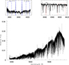 |
Fig. 1. Spectrum from the SOPHIE database for GJ 617A. A zoomed-in view highlights the Ca II K (in emission) with a dashed blue line and the Hα lines with a dashed red line, along with the Hα region. |
The first stage of our methodology focused on evaluating and filtering the spectra based on their signal-to-noise ratio (S/N). To ensure reliable measurements of the activity indices, specific S/N thresholds were defined at the wavelengths relevant to each indicator. In particular, we retained only spectra with S/N > 50 measured in order 38, which contains the Ca II H and K lines. As a result of this filtering, approximately 45 spectra were discarded for GJ 617A and about 15 spectra for GJ 411.
In addition to the spectral quality criterion, we focused on selecting stars with time series long enough to allow the detection of robust stellar cycles. Following the statistics presented by Suárez Mascareño et al. (2016), we adopted a minimum observational baseline of seven years. This criterion allowed us to align our sample selection with the known distribution of activity cycles in M dwarfs Suárez Mascareño et al. (2018), ensuring that the longer stellar periods typical of this type of star can be reliably detected.
The SOPHIE observations analysed in this work span 2008–2024 for GJ 617A and 2007–2024 for GJ 411, providing a sufficiently long temporal baseline to investigate stellar magnetic activity on long timescales.
3. Long-term activity analysis
To detect long-term activity cycles or systematic variations in M dwarf stars, both with and without planetary companions, we first constructed time series of activity proxies. Taking advantage of the broad wavelength coverage of SOPHIE spectra, we analysed simultaneous measurements of Hα and Ca II stellar activity indices. To do so, we computed dimensionless activity indices in both lines following Cincunegui et al. (2007). The Ca II index, hereafter S-index, is computed as the ratio between the mean H and K line-core fluxes integrated with a triangular profile with a full width at half maximum of 1.09 Å (see Fig. 1) to the mean continuum nearby integrated over two windows of 20 Å centred at m 4001 and 3901 Å. The Hα-index is defined as the ratio of the average line-core flux integrated with a rectangular band of a width of 0.7 Å (see Fig. 1) centred at 6592.8 Å and the average flux or number of counts in the continuum nearby centred at 6605 Å and with a width of 20 Å.
To clean the time series of the activity indices from any outliers or flares (Fig. 15; see Sect. 5.2 for more details) that might affect the accuracy of the results, we first computed a moving mean with a 90-day window. Outlier detection was based on a 2σ threshold from this smoothed curve. In cases where outliers were identified, they were removed if their values were significantly above the typical range of the series, thus allowing the analysis to focus on stellar activity associated with long-term phenomena, such as starspots or faculae. To preserve the temporal coherence of the datasets, all measurements rejected from the time series of a given activity index were also removed from the time series of the other index.
A total of 480 spectra were available for GJ 617A, of which 23 were identified as outliers and excluded, resulting in 457 spectra used in the final analysis. For GJ 411, 341 spectra were available, with 57 identified and excluded as outliers, leaving 284 spectra for the final time series.
Finally, we proceeded with the analysis aimed at identifying long-term stellar activity cycles. To this end, we applied two complementary approaches based on the standard generalised Lomb–Scargle (GLS) periodogram (Zechmeister & Kürster 2009). The classical GLS models the data using a purely sinusoidal basis and assumes a constant baseline, an assumption that may not hold in the presence of slow non-sinusoidal variability or long-term trends.
To relax this constraint, we adopted an extended formulation of the GLS, hereafter referred to as LinGLS (linear generalised Lomb–Scargle), which augments the harmonic basis with a low-order polynomial component. This approach allows simultaneous modelling of periodic signals and long-term variations, and it is particularly well suited for irregularly sampled time series affected by secular trends.
We denote by  the observation times and corresponding chromospheric activity measurements, with associated uncertainties σi. A constant uncertainty was adopted for all data points, justified by the instrumental stability of the activity index. Long-term variations were modelled using a second-order polynomial basis,
 (1)
(1)
where  is the mean observation time.
An initial fit using only the polynomial component yielded a reference model and a reduced chi-square, χ02. For each trial frequency, ν, drawn from a densely sampled frequency grid defined by the temporal baseline and an oversampling factor, the design matrix was extended to include sinusoidal terms:
![Mathematical equation: $$ \begin{aligned} \Phi _{\nu }(t_i) = \left[ \Phi _{\mathrm{poly} }(t_i), \; \sin (2\pi \nu t_i), \; \cos (2\pi \nu t_i) \right]. \end{aligned} $$](/articles/aa/full_html/2026/04/aa56087-25/aa56087-25-eq4.gif) (2)
(2)
The full model,
 (3)
(3)
was fitted by weighted linear least squares, and we solved the normal equations via Cholesky decomposition and included a small regularisation term of 10−8 to ensure numerical stability. The reduced chi-square χ2(ν) was computed for each frequency.
The LinGLS power was defined as
 (4)
(4)
such that high values of P(ν) indicate a significant improvement of the fit when including a periodic component at frequency ν.
By explicitly modelling long-term trends, LinGLS avoids biases associated with a constant baseline assumption and reduces sensitivity to slow instrumental or astrophysical variations. This makes it particularly well suited for the analysis of chromospheric activity indices in M dwarfs, whose variability often departs from simple sinusoidal behaviour.
To further exploit the information provided by the LinGLS framework, we analysed the statistical significance of the polynomial coefficients associated with the dominant frequency identified in the periodograms. For both GJ 411 and GJ 617A, we performed an ordinary least-squares fit of a sinusoidal model combined with polynomial terms to the activity indices, fixing the frequency to that of the main periodogram peak.
All data points were assigned equal weights, which is equivalent to an unweighted fit. The statistical significance of each coefficient was then evaluated using Student’s t-test, and the results were summarised using standard significance levels.
We estimated the false alarm probabilities (FAPs) using a bootstrap re-sampling method. The FAP for an observed periodogram power, P, was determined using a bootstrap re-sampling approach. We generated 10 000 synthetic time series by resampling the original data (or residuals) under the null hypothesis of no periodicity. The periodogram was computed for each synthetic series. The FAP was then calculated as the fraction of these synthetic periodograms that showed a maximum power equal to or greater than the observed power, P.
4. Magnetic activity cycles in GJ 617A and GJ 411
Based on the GLS and LinGLS periodograms described above, we identified stars exhibiting clear periodic signals with a false-alarm probability (FAP) below 1%. In other cases, the periodograms showed no significant periodicity or variability.
4.1. GJ 617A – HD147379A – HIP 79755
The M dwarf star GJ 617A (HD147379A, HIP 79755, J16167+672S) is a bright star classified as M0V (Alonso-Floriano 2015), and it is located at a distance of d = 10.767 ± 0.002 pc (Gaia Collaboration 2023); further details are provided in Table 1. This star forms a common proper motion pair with a fainter companion (GJ 617B, a BY Dra variable) at a projected separation of 1.07 arcminutes, or approximately 690 AU at the system distance (Stalport et al. 2023). Rotational broadening was detected in CARMENES data (Reiners et al. 2018), which permitted measurement of the projected rotational velocity: v sin i = 2.7 ± 1.5 km s−1.
Key stellar parameters of GJ 617A and GJ 411.
In terms of stellar activity, GJ 617A exhibits weak chromospheric emission in Ca II H and K, with a mean S-index of 1.53 derived from HIRES data (Butler et al. 2017). Although Butler et al. reported the absence of Hα emission in most of their spectra, CARMENES data indicated that Hα is observed in absorption. In contrast, Newton et al. (2017) detected Hα emission in GJ 617A, which differs from previous findings, while Gizis et al. (2002) also recorded Hα in absorption. This discrepancy reflects the complexity of chromospheric processes in GJ 617A.
Reiners et al. (2018) estimated the star’s rotation period to be approximately P ≈ 31 days based on the relationship between X-ray activity and rotational period from Reiners et al. (2014). The uncertainty in this estimate is about ±20 days, as the X-ray values of individual stars show considerable scatter around the activity-rotation relationship.
According to Jeffers et al. (2018), stars with rotation periods of 10 days or longer (Prot ≥ 10 days) typically lack Hα emission, indicating low activity levels, whereas faster rotators (Prot < 10 days) usually exhibit Hα emission and are therefore considered active. Hobson et al. (2018) confirmed the presence of an exoplanet previously reported using CARMENES data by Reiners et al. (2018). This planet, GJ 617Ab, has an orbital period of 86.7 days and a minimum mass of 31.29 Earth masses, and is potentially located within the habitable zone near its inner boundary. By combining observations from multiple facilities, Hobson et al. (2018) further refined the planetary parameters. In this joint analysis, the previously reported ∼500-day signal was not confirmed, indicating that it was likely spurious.
Figure 2 illustrates the evolution of the S-index. The vertical axis shows the S-index, with a mean value of 1.27 and a standard deviation of 0.06. Figure 3 shows the temporal variation of the Hα index over 10 years (2014–2024) using the same timescale as the S-index series. Flares should have been removed with the procedure outlined in previous section.
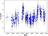 |
Fig. 2. Time series of the S-index for GJ 617A. Each point represents a SOPHIE spectrum. |
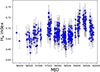 |
Fig. 3. Time series of the Hα index for GJ 617A. Each point represents the spectra (data) obtained with the SOPHIE spectrograph. |
The two indicators, the S and Hα indices, exhibit similar variation patterns over time, suggesting a good correlation between them, with a Pearson correlation coefficient of R = 0.75. This is further quantified in Fig. 8, which presents the correlation between the successive differences in the Hα and S-index activity indicators with R = 0.73.
Subsequently, to search for long-term activity cycles, we computed the GLS and Lin-GLS periodograms. Figures 4 and 5 each present both periodograms superimposed corresponding to the S-index and the Hα index. In the figures, prominent peaks indicate potential activity cycles. One of these peaks, corresponding to a cycle of approximately 1800 days, stands out in both models, suggesting the presence of a clear and significant cycle in both indicators (i.e. the S and Hα indices). When a long-term variation is accounted for simultaneously with the Lin-GLS model, the peaks are found at around 1700 days. All reported periods were obtained considering a FAP threshold of less than 10−4.
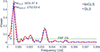 |
Fig. 4. Generalised Lomb–Scargle (blue) and LinGLS (red) periodograms of GJ 617A using the S-index. The main peaks are at (1831.67 ± 838.75) d (GLS) and (1752.03 ± 767.40) d (LinGLS). |
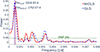 |
Fig. 5. Generalised Lomb–Scargle (blue) and LinGLS (red) periodograms of GJ 617A using the Hα index. The main peaks are at (1918.93 ± 920.57) d (GLS) and (1752.07 ± 767.43) d (LinGLS). |
To further examine this periodicity, we constructed phase-folded time series at this period. These are shown in Fig. 6 regarding the S-index and Fig. 7 for the Hα index, where a sinusoidal model is overplotted. Although the phase-folded series may give the visual impression of a phase offset between the two indices, our statistical analysis indicates that they are in fact positively correlated (Pearson R = 0.75 for the raw indices and R = 0.73 for successive differences; see Fig. 8). We therefore do not interpret the apparent visual offset as evidence of anti-phase behaviour.
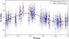 |
Fig. 6. Variability on GJ 617A. Phase-folded time series of the S activity index versus phase, with datasets indicated by blue circles and the best-fit harmonic curve shown in red. The phase folding was performed using the period obtained from the GLS analysis. |
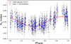 |
Fig. 7. Variability on GJ 617A. The phase-folded time series Hα activity index versus the phase of the datasets is indicated with blue circles. The harmonic curve that best fits the data is in red. The phase folding was performed using the period obtained from the GLS analysis. |
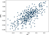 |
Fig. 8. Correlation between the successive differences in the Hα and S-index activity indicators for GJ 617A. The Pearson correlation coefficient is R = 0.73. |
4.2. GJ 411 – HD 95735 – Lalande 21185
The star Gliese 411, also known as Lalande 21185 or HD95735, is one of the closest M dwarfs to the Solar System. Its physical parameters are given in Table 1. Over the years, this star has been a primary target in the search for exoplanets. Early astrometric studies suggested the possible presence of a planetary companion, but these claims were never confirmed. More recent RV studies have provided a clearer view of the system.
Butler et al. (2017) detected a periodic signal of 9.9 days, which they attributed to a planet, GJ 411b. However, Díaz et al. (2019) and later Stock et al. (2020) identified a more robust signal with a 12.95-day period, corresponding to a super-Earth with a minimum mass of 3.8 M⊕. Stock et al. (2020) also identified a periodicity of ∼2900 days, initially interpreted as a magnetic activity cycle, although Rosenthal et al. (2021) subsequently attributed it to a second planet, GJ 411c.
The study by Hurt et al. (2022) confirms the existence of the long-period planet GJ 411c. The authors also report a 200-day signal whose nature could not clearly be established. This candidate signal has yet to be definitively confirmed, but it shows promising signs of being a genuine exoplanet.
This work is based on 284 SOPHIE spectra acquired between 2008 and 2024. Figure 9 shows the time series for the S-index of GJ 411, which has a mean value of ⟨S⟩ = 0.65 and a standard deviation of 0.09. We show the time series for the Hα index in Fig. 10. We observed that the temporal behaviour of the S-index and Hα index do not exhibit a correlation over time, indicating distinct patterns in their respective time series.
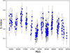 |
Fig. 9. Time series of the S-index for GJ 411. Each point represents the spectra (data) obtained with the SOPHIE spectrograph. |
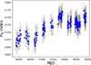 |
Fig. 10. Time series of the Hα index for GJ 411. Each point represents the spectra (data) obtained with the SOPHIE spectrograph. |
Following a similar methodology for GJ 617A, we built the corresponding periodograms for both activity indicators. In Fig. 11 we show the resulting periodograms for the S-index. A significant peak was found at 688.02 days using the GLS method and at 665.46 days using the LinGLS method.
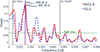 |
Fig. 11. Generalised Lomb–Scargle (blue) and LinGLS (red) periodograms of GJ 411 using the S-index. The main peaks are at (688.02 ± 118.34) d (GLS) and (665.46 ± 110.70) d (LinGLS). The vertical black lines mark the orbital period of GJ 411c (∼2900) and an additional signal around 200 d. |
To explore the low-frequency domain where Stock et al. (2020) announced the additional companion, we subtracted a harmonic function of the period detected from each time series. This allowed for the identification of a second significant peak: 386 days in the GLS periodogram and 2136 days in the LinGLS periodogram (as shown in Fig. 12).
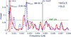 |
Fig. 12. Generalised Lomb–Scargle (blue) and LinGLS (red) periodograms of GJ 411 using the S-index after subtracting a harmonic of the detected period. The main peaks are at (386.6 ± 37.36) d (GLS) and (2136.48 ± 1141.13) d (LinGLS). The vertical black lines mark the orbital period of GJ 411c (∼2900 d) and an additional signal around 200 d. |
This analysis reveals that the quadratic polynomial term is statistically significant only in the case of GJ 411, while it is not required to describe the variability of GJ 617A. This result provides a quantitative explanation for the differences observed between the standard GLS and LinGLS periodograms. The activity indicators of GJ 411 exhibit long-term variations that cannot be characterised by a purely sinusoidal model. Such behaviour points to complex non-sinusoidal variability or secular trends consistent with a long-period magnetic cycle in evolution or a transition towards a broad minimum or due to a Waldmeier effect, which has been observed in other cool stars (Robertson et al. 2013; Buccino et al. 2020; Flores Trivigno et al. 2024). Consequently, long-term RV and activity monitoring over decadal timescales are required to characterise the nature of this stellar activity.
We also performed a periodogram analysis for the Hα index (see Fig. 13). A low-frequency rise was observed, as expected from the appearance of the time series. In the Ca II-index, the dominant signal appears at 2136 days, whereas in the Hα index, the most significant period is approximately 1624 days. The latter suggests the presence of a long-term activity cycle that is not consistently detected in both indices. These differences highlight that the dominant periodicities inferred from different activity indicators may vary, as also reported by Mignon et al. (2023) for several M dwarfs.
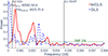 |
Fig. 13. Generalised Lomb–Scargle (blue) and LinGLS (red) periodograms of GJ 411 using the Hα index. The main peaks are at (40592.50 ± 411.94) d (GLS) and (1623.7 ± 659.10) d (LinGLS). The vertical black lines mark the orbital period of GJ 411c (∼2900 d) and an additional signal around 200 d. |
4.3. Stellar population membership for GJ 411 and GJ 617A
Using proper motions and parallaxes from Gaia DR3 (Gaia Collaboration 2018), we derived the Galactic space-velocity UVW components for both stars by following the procedure detailed in Jofré et al. (2015). We find that (U, V, W) = (−56.08, −48.56, −67.10) km s−1 for GJ 411 and (U, V, W) = (−0.35, −24.95, 11.46) km s−1 for GJ 617A.
Then, based on these space-velocity components and using the membership formulation of Reddy et al. (2006), we determined that the probability of belonging to the thin-disc population is ∼98% for GJ 617A. The UVW values for GJ 411 are consistent with thick-disc membership, with a probability of ∼93%.
5. Searching for hints of short-term photometric activity in TESS data
The Transiting Exoplanet Survey Satellite (Ricker et al. 2015) is a NASA space mission launched in 2018 whose main purpose is to look for and characterise transiting planets around bright and nearby stars. However, thanks to its high-cadence observing modes, TESS observations are also valuable for detecting stellar variability, including pulsations, rotational modulation, and flares. Therefore, as a complement to the long-term spectroscopic study, we used photometric datasets from TESS to characterise the short-term variability of the two stars. Furthermore, simultaneous photometry and activity indices help determine whether stellar activity is dominated by spots with cooler surface features, which make stars redder when fainter, or by plages, which make stars bluer with higher activity (Hall et al. 2009)
5.1. Rotation period
The stars GJ 411 and GJ 617A were observed by TESS in several sectors with multiple cadences. Table 2 provides a summary of these observations. For both stars, we used the tools available in the LIGHTKURVE Python package (Lightkurve Collaboration 2018) to analyse the light curves resulting from the pre-search data conditioning simple aperture photometry (PDCSAP) data processed with the TESS Science Processing Operations Center (SPOC) pipeline (Jenkins et al. 2016). After removing bad points, we ran a GLS periodogram to search for signs of sinusoidal modulation. The rotation period, Prot, was determined as the inverse of the frequency with the highest peak found by GLS. To ensure that Prot was reliable, we required it to satisfy the following conditions:
-
False alarm probability (FAP) ≤0.01.
-
The standard deviation of the residuals after removing the periodic signal is smaller than or, at most, equal to the light curve’s standard deviation before removing the sinusoidal modulation.
-
More than 50% of the available cadences show the period value identified by GLS.
-
After a careful by-eye inspection, variability is visible in the phase-folded light curve.
-
The value of the period found differs from the duration of a sector, the duration of half a sector, and the duration of the full light curve.
Summary of TESS observations.
For GJ 411, before eliminating bad points, it was necessary to apply a median filter to the photometric data to eliminate the still present systematics. For this target, none of the detected signals turned out to be significant, and hence there is no evidence of rotational variability in the TESS data analysed. The absence of a clear detection is consistent with the ongoing uncertainty in the literature surrounding the true rotation period of GJ 411. For instance, Díaz et al. (2019) proposed a rotation period of 56 days based on photometric variations. However, more recent analyses using SPIRou spectropolarimetric data have yielded unusual results: Donati et al. (2023) report a strange and poorly understood modulation with a period of 427 days, while Fouqué et al. (2023) propose a very long rotation period of 478 days based on variations in the longitudinal magnetic field (Bl).
In contrast, for GJ 617A, we found a reliable rotation period of 10.412 ± 0.055 days with a photometric amplitude of Amp = 0.0001 mag in the 2-min cadence data considering 38 TESS sectors. Inside errors, Prot values were also found after running the GLS periodogram on the 200s, 1800s, and 20s cadence TESS light curves. The 600s cadence was the only one that showed a different peak value in the periodogram. The Prot value around 10 days detected in our analysis agrees with the first harmonic found in previous works using spectroscopic data (Hobson et al. 2018; Reiners et al. 2018) and 28 sectors of TESS photometry (Stalport et al. 2023). In this study, we did not recover the ∼21-day signal found by Stalport et al. (2023). One possible reason is that in this work, we used PDCSAP data already corrected by systematics, while in Stalport et al. (2023), the authors employed simple aperture photometry data and performed their own de-trending to eliminate the systematics. In Fig. 14 we present the phase-folded 2-min cadence light curve considering a period of 10.4 days and the corresponding GLS periodogram.
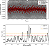 |
Fig. 14. TESS photometric rotation signature of GJ 617A. Top panel: Zoom-in view of the phase-folded 2-min cadence TESS light curve of GJ 617A considering a period of 10.4 days. Grey and red symbols indicate the 2-min cadence and 1-day binned TESS data, respectively. The solid line represents the best sinusoidal fit to the data. Bottom panel: GLS periodogram of the 1-day binned 2-min cadence TESS light curve. Horizontal lines indicate different FAP values. |
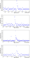 |
Fig. 15. Examples of flare events found in GJ 617A. |
Finally, we explored whether the rotation period values measured in each individual TESS sector evolve along with the minimum and maximum values of the S and Hα indices. After running a GLS periodogram on the data and a thorough visual inspection, no correlation was found between the short- and long-term variability.
5.2. Flares
To look for flaring events in the stars, we followed the methodology implemented in previous works (Petrucci et al. 2024; Martioli et al. 2024). First, a Savitzky-Golay filter with an optimum value of window length (wl = 1) was applied to the TESS light curve to remove systematics and intrinsic stellar variability. Then, the ALTAIPONY code (Davenport 2016; Ilin et al. 2021) was used to identify flare candidates. We repeated the same process in all the available sectors and cadences. Bona fide flares were then confirmed after a careful by-eye inspection, and their bolometric energy, Ebol, was computed as indicated in Eq. (1) of Petrucci et al. (2024). As an additional check, we examined if these bona fide events were detected in the same sector at different cadences.
We found no signs of flaring activity in the TESS light curve of GJ 411. For GJ 617A, we identified nine flare events with bolometric energies ranging from 3.44 × 1033 erg s−1 to 4.93 × 1032 erg s−1.
6. Summary and conclusions
M dwarfs play a crucial role in exoplanet research, as their small sizes and low luminosities make them particularly favourable for the detection of Earth-sized planets within their HZs. Nonetheless, their intrinsic stellar activity – manifested through phenomena such as flares, rotational modulation, and long-term activity cycles – introduces significant challenges for both the detection of planetary signals and the characterisation of exoplanetary atmospheres.
With this in mind, in the present work, we characterised the stellar activity of two early M stars with planets, GJ 617A and GJ 411, based on 13 years of SOPHIE data. For GJ 617A, we built an S and Hα index time series. From analysis with different periodograms, we reported for the first time a ∼1800-day periodic signal. The observed periodicity in both indices suggests a coherent magnetic cycle that influences multiple atmospheric layers. The positive correlation between both incremental indices, R = 0.75, is consistent with the distribution of the correlation coefficients with activity observed in Fig. 6 in Meunier et al. (2024).
Although GJ 411 is a very inactive star, the nature of the long-term periodicities observed in its RV variations – whether of planetary origin or linked to stellar activity – remains a topic of debate (Stock et al. 2020; Rosenthal et al. 2021; Hurt et al. 2022). Here, we analysed simultaneous observations of Hα and calcium indices between 2011 and 2024. Our analysis revealed a primary periodicity of 688 days and a secondary long-term variability of 2136 and 1623 days in both indices, respectively. We are not certain about the origin of the 688-day signal. Because the signal is seen on a single activity index, we tentatively attribute it to a combination of a long-term variation aliasing with the window function. Furthermore, the current understanding of activity cycles disfavours cycles with such a short periodicity on low-activity-level stars. This finding underscores the complexity of the underlying dynamo processes in GJ 411.
The detected long-term activity periods are summarised in Table 3. From the mean S-index of the SOPHIE dataset for each star, we computed  values using the calibration of Boisse et al. (2010) for the V − K colour together with the corresponding coefficients from Astudillo-Defru et al. (2017) (see Table 3).
Results of the long-term activity cycle analysis obtained in this work.
Based on their kinematic properties, we classified GJ 617A as a thin-disc star and GJ 411 as a member of the Galactic thick disc. The difference in activity regimes can be partially explained by the rotational evolution of M dwarfs. As stars age, they lose angular momentum through magnetic braking, leading to progressively slower rotation. This reduced rotation rate decreases the efficiency of the dynamo mechanism and thus lowers the observable level of magnetic activity. Therefore, the very low level of stellar activity observed in GJ 411 – evidenced by the absence of flares and rotational modulation in photometric data, as well as weak variability in the chromospheric Hα and Ca II H and K indices – is consistent with the old age associated with the thick-disc population (≳10–11 Gyr; Bensby et al. 2005; Reddy et al. 2006; Adibekyan et al. 2011).
To complement this long-term study, we performed a short-term analysis using high-cadence TESS photometry (see Table 2). For GJ 411, we did not detect any appreciable short-term photometric variability and therefore do not confirm the rotation period of 56 days reported in previous studies.
In contrast, the TESS photometry of GJ 617A reveals a sinusoidal modulation with a period of 10.412 days, which we associate with the first harmonic of its rotation period of 22 days. Additionally, we identify several stochastic events attributable to flares, with energies ranging from 1 × 1033 erg s−1 to 4.93 × 1032 erg s−1.
None of the detected periods for these stars coincide with the previously reported planetary signals. This suggests that the variations observed in the activity indicators are associated with magnetic variability driven by stellar dynamo processes, thus strengthening the validity of the published planetary detections.
In order to analyse these long-term cycles in the stellar context, we placed our results in the empirical diagram Pcyc − Prot built for solar-type stars in Metcalfe et al. (2016), see Fig. 16. Furthermore, we included the activity cycles of early and mid-M dwarfs also reported in the literature (Buccino et al. 2011; Ibañez Bustos et al. 2020, 2025). In Fig. 16, it is remarkable that GJ 617A falls in the branch associated with inactive solar-type stars. This may give the idea that rotation drives the magnetic dynamo in GJ 617A. On the other hand, the cycles detected for GJ 411 do not fall close to any branch in the diagram. This behaviour seems to be similar to other early M star slow-rotators such as GJ 229 or GJ 536.
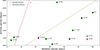 |
Fig. 16. Activity period (days) versus rotation period (days). The dashed red lines represent the active branch (A), while the dashed olive lines represent the inactive branch (I). These lines were taken from the work of Metcalfe et al. (2016) and were computed for solar-type stars. The green dots correspond to some M-type stars. Blue diamonds represent the results obtained in this work based on the S-index, and red diamonds correspond to results obtained based on the Hα index. |
In summary, we have presented a long-term analysis of stellar activity based on a homogeneous dataset for two early M-type dwarf stars: GJ 617A and GJ 411. Although the stellar interiors of the stars exhibit similar physical characteristics and structure, the stars differ significantly in their rotational and magnetic activity properties. GJ 411 is a slowly rotating inactive star, whereas GJ 617A is a moderately rotating flare star. The long-term variability observed in GJ 617A seems to be consistent with a solar-like dynamo mechanism. In contrast, the activity periodicities detected in GJ 411 deviate from the usual semi-empirical relations established for solar-type stars. If these signals are attributed to stellar cycles, this observation would suggest the presence of a different type of dynamo process – likely one in which convective dynamics play a dominant role.
Acknowledgments
We warmly thank the OHP staff for their support on the observations. IB received funding from the French Programme National de Physique Stellaire (PNPS) and the Programme National de Planétologie (PNP) of CNRS (INSU). R.P. and E.J. acknowledge funding from CONICET, under projects PIBAA-CONICET ID-73811 and ID-73669. Funding for the TESS mission is provided by NASA’s Science Mission Directorate. We acknowledge the use of public TESS data from pipelines at the TESS Science Office and at the TESS Science Processing Operations Center. Resources supporting this work were provided by the NASA High-End Computing (HEC) Program through the NASA Advanced Supercomputing (NAS) Division at Ames Research Center for the production of the SPOC data products. Data presented in this paper were obtained from the Mikulski Archive for Space Telescopes (MAST). This work has made use of data from the European Space Agency (ESA) mission Gaia (https://www.cosmos.esa.int/gaia), processed by the Gaia Data Processing and Analysis Consortium (DPAC, https: //www.cosmos.esa.int/web/gaia/dpac/consortium). Funding for the DPAC has been provided by national institutions, in particular the institutions participating in the Gaia Multilateral Agreement. C. G. O. also wishes to express their heartfelt gratitude to Hilda E. Jara for her unconditional support throughout this work, and to C.A.S.L.A., her great passion.
References
- Adibekyan, V. Z., Santos, N. C., Sousa, S. G., & Israelian, G. 2011, A&A, 535, L11 [NASA ADS] [CrossRef] [EDP Sciences] [Google Scholar]
- Alonso-Floriano, F. J. 2015, Ph.D. Thesis, Complutense University of Madrid, Department of Astronomy, Spain [Google Scholar]
- Anglada-Escudé, G., Amado, P. J., Barnes, J., et al. 2016, Nature, 536, 437 [Google Scholar]
- Astudillo-Defru, N., Delfosse, X., Bonfils, X., et al. 2017, A&A, 600, A13 [NASA ADS] [CrossRef] [EDP Sciences] [Google Scholar]
- Baliunas, S. L., Donahue, R. A., Soon, W. H., et al. 1995, ApJ, 438, 269 [Google Scholar]
- Baycroft, T. A., Santerne, A., Triaud, A. H. M. J., et al. 2025, MNRAS, 541, 2801 [Google Scholar]
- Bensby, T., Feltzing, S., Lundström, I., & Ilyin, I. 2005, A&A, 433, 185 [NASA ADS] [CrossRef] [EDP Sciences] [Google Scholar]
- Bochanski, J. J., Hawley, S. L., Covey, K. R., et al. 2010, AJ, 139, 2679 [NASA ADS] [CrossRef] [Google Scholar]
- Boisse, I., Eggenberger, A., Santos, N. C., et al. 2010, A&A, 523, A88 [NASA ADS] [CrossRef] [EDP Sciences] [Google Scholar]
- Boisse, I., Bouchy, F., Hébrard, G., et al. 2011, A&A, 528, A4 [NASA ADS] [CrossRef] [EDP Sciences] [Google Scholar]
- Boisse, I., Pepe, F., Perrier, C., et al. 2012, A&A, 545, A55 [NASA ADS] [CrossRef] [EDP Sciences] [Google Scholar]
- Bonfils, X., Delfosse, X., Udry, S., et al. 2013, A&A, 549, A109 [NASA ADS] [CrossRef] [EDP Sciences] [Google Scholar]
- Bouchy, F., Hébrard, G., Udry, S., et al. 2009, A&A, 505, 853 [NASA ADS] [CrossRef] [EDP Sciences] [Google Scholar]
- Bouchy, F., Hébrard, G., Delfosse, X., et al. 2011, in EPSC-DPS Joint Meeting 2011, 2011, 240 [NASA ADS] [Google Scholar]
- Bouchy, F., Díaz, R. F., Hébrard, G., et al. 2013, A&A, 549, A49 [NASA ADS] [CrossRef] [EDP Sciences] [Google Scholar]
- Buccino, A. P., Díaz, R. F., Luoni, M. L., Abrevaya, X. C., & Mauas, P. J. D. 2011, AJ, 141, 34 [NASA ADS] [CrossRef] [Google Scholar]
- Buccino, A. P., Sraibman, L., Olivar, P. M., & Minotti, F. O. 2020, MNRAS, 497, 3968 [NASA ADS] [CrossRef] [Google Scholar]
- Butler, R. P., Vogt, S. S., Laughlin, G., et al. 2017, AJ, 153, 208 [Google Scholar]
- Cifuentes, C., Caballero, J. A., Cortes-Contreras, M., et al. 2020, VizieR On-line Data Catalog: J/A+A/642/A115 [Google Scholar]
- Cincunegui, C., Díaz, R. F., & Mauas, P. J. D. 2007, A&A, 469, 309 [NASA ADS] [CrossRef] [EDP Sciences] [Google Scholar]
- Cortes-Zuleta, P., Boisse, I., Ould-Elhkim, M., et al. 2024, VizieR On-line Data Catalog: J/A+A/693/A164 [Google Scholar]
- Davenport, J. R. A. 2016, ApJ, 829, 23 [Google Scholar]
- Demangeon, O. D. S., Dalal, S., Hébrard, G., et al. 2021, A&A, 653, A78 [NASA ADS] [CrossRef] [EDP Sciences] [Google Scholar]
- Díaz, R. F., Ramírez, S., Fernández, J. M., et al. 2007, ApJ, 660, 850 [CrossRef] [Google Scholar]
- Díaz, R. F., Rey, J., Demangeon, O., et al. 2016, A&A, 591, A146 [Google Scholar]
- Díaz, R. F., Delfosse, X., Hobson, M. J., et al. 2019, A&A, 625, A17 [NASA ADS] [CrossRef] [EDP Sciences] [Google Scholar]
- Donati, J. F., Lehmann, L. T., Cristofari, P. I., et al. 2023, MNRAS, 525, 2015 [CrossRef] [Google Scholar]
- Dumusque, X., Lovis, C., Ségransan, D., et al. 2011a, A&A, 535, A55 [NASA ADS] [CrossRef] [EDP Sciences] [Google Scholar]
- Dumusque, X., Santos, N. C., Udry, S., Lovis, C., & Bonfils, X. 2011b, A&A, 527, A82 [NASA ADS] [CrossRef] [EDP Sciences] [Google Scholar]
- Flores Trivigno, M., Buccino, A. P., González, E., et al. 2024, A&A, 691, L6 [NASA ADS] [CrossRef] [EDP Sciences] [Google Scholar]
- Flores, M., González, J. F., Jaque Arancibia, M., et al. 2018, A&A, 620, A34 [NASA ADS] [CrossRef] [EDP Sciences] [Google Scholar]
- Fouqué, P., Martioli, E., Donati, J. F., et al. 2023, A&A, 672, A52 [NASA ADS] [CrossRef] [EDP Sciences] [Google Scholar]
- Fuhrmeister, B., Czesla, S., Hildebrandt, L., et al. 2020, A&A, 640, A52 [NASA ADS] [CrossRef] [EDP Sciences] [Google Scholar]
- Gaia Collaboration (Katz, D., et al.) 2018, A&A, 616, A11 [NASA ADS] [CrossRef] [EDP Sciences] [Google Scholar]
- Gaia Collaboration (Vallenari, A., et al.) 2023, A&A, 674, A1 [NASA ADS] [CrossRef] [EDP Sciences] [Google Scholar]
- Gizis, J. E., Reid, I. N., & Hawley, S. L. 2002, AJ, 123, 3356 [Google Scholar]
- Gomes da Silva, J., Santos, N. C., Bonfils, X., et al. 2011, A&A, 534, A30 [NASA ADS] [CrossRef] [EDP Sciences] [Google Scholar]
- Gomes da Silva, J., Santos, N. C., Bonfils, X., et al. 2012, A&A, 541, A9 [NASA ADS] [CrossRef] [EDP Sciences] [Google Scholar]
- Gomes da Silva, J., Santos, N. C., Boisse, I., Dumusque, X., & Lovis, C. 2014, A&A, 566, A66 [NASA ADS] [CrossRef] [EDP Sciences] [Google Scholar]
- Gomes da Silva, J., Bensabat, A., Monteiro, T., & Santos, N. C. 2022, A&A, 668, A174 [NASA ADS] [CrossRef] [EDP Sciences] [Google Scholar]
- Hall, J. C., Henry, G. W., Lockwood, G. W., Skiff, B. A., & Saar, S. H. 2009, AJ, 138, 312 [NASA ADS] [CrossRef] [Google Scholar]
- Hara, N. C., Bouchy, F., Stalport, M., et al. 2020, A&A, 636, L6 [NASA ADS] [CrossRef] [EDP Sciences] [Google Scholar]
- Hébrard, G., Bonfils, X., Ségransan, D., et al. 2010, A&A, 513, A69 [NASA ADS] [CrossRef] [EDP Sciences] [Google Scholar]
- Heidari, N., Boisse, I., Hara, N. C., et al. 2024, A&A, 681, A55 [NASA ADS] [CrossRef] [EDP Sciences] [Google Scholar]
- Hobson, M. J., Díaz, R. F., Delfosse, X., et al. 2018, A&A, 618, A103 [NASA ADS] [CrossRef] [EDP Sciences] [Google Scholar]
- Hurt, S. A., Fulton, B., Isaacson, H., et al. 2022, AJ, 163, 218 [Google Scholar]
- Ibañez Bustos, R. V., Buccino, A. P., Flores, M., & Mauas, P. J. D. 2019, A&A, 628, L1 [NASA ADS] [CrossRef] [EDP Sciences] [Google Scholar]
- Ibañez Bustos, R. V., Buccino, A. P., Messina, S., Lanza, A. F., & Mauas, P. J. D. 2020, A&A, 644, A2 [NASA ADS] [CrossRef] [EDP Sciences] [Google Scholar]
- Ibañez Bustos, R. V., Buccino, A. P., Flores, M., Martinez, C. F., & Mauas, P. J. D. 2023, A&A, 672, A37 [NASA ADS] [CrossRef] [EDP Sciences] [Google Scholar]
- Ibañez Bustos, R. V., Buccino, A. P., Nardetto, N., et al. 2025, A&A, 696, A230 [NASA ADS] [CrossRef] [EDP Sciences] [Google Scholar]
- Ilin, E., Schmidt, S. J., Poppenhäger, K., et al. 2021, A&A, 645, A42 [NASA ADS] [CrossRef] [EDP Sciences] [Google Scholar]
- Jeffers, S. V., Schöfer, P., Lamert, A., et al. 2018, A&A, 614, A76 [NASA ADS] [CrossRef] [EDP Sciences] [Google Scholar]
- Jenkins, J. M., Twicken, J. D., McCauliff, S., et al. 2016, SPIE Conf. Ser., 9913, 99133E [Google Scholar]
- Jofré, E., Petrucci, R., Saffe, C., et al. 2015, A&A, 574, A50 [Google Scholar]
- Kar, A., Henry, T. J., Couperus, A. A., Vrijmoet, E. H., & Jao, W. C. 2024, VizieR On-line Data Catalog: J/AJ/167/196 [Google Scholar]
- Kopparapu, R. K., Ramirez, R., Kasting, J. F., et al. 2013, ApJ, 765, 131 [NASA ADS] [CrossRef] [Google Scholar]
- Lafarga, M., Ribas, I., Reiners, A., et al. 2021, VizieR On-line Data Catalog: J/A+A/652/A28. [Google Scholar]
- Leenaarts, J., Carlsson, M., & Rouppe van der Voort, L. 2012, ApJ, 749, 136 [NASA ADS] [CrossRef] [Google Scholar]
- Lehmann, L. T., Donati, J. F., Fouqué, P., et al. 2024, MNRAS, 527, 4330 [Google Scholar]
- Lightkurve Collaboration (Cardoso, J. V. d. M., et al.) 2018, Astrophysics Source Code Library [record ascl:1812.013] [Google Scholar]
- Lovis, C., Ségransan, D., Mayor, M., et al. 2011, A&A, 528, A112 [NASA ADS] [CrossRef] [EDP Sciences] [Google Scholar]
- Martin, J., Fuhrmeister, B., Mittag, M., et al. 2017, A&A, 605, A113 [NASA ADS] [CrossRef] [EDP Sciences] [Google Scholar]
- Martioli, E., Petrucci, R. P., Jofré, E., et al. 2024, A&A, 690, A312 [NASA ADS] [CrossRef] [EDP Sciences] [Google Scholar]
- Mauas, P. J. D., & Falchi, A. 1994, A&A, 281, 129 [NASA ADS] [Google Scholar]
- Mauas, P. J. D., & Falchi, A. 1996, A&A, 310, 245 [NASA ADS] [Google Scholar]
- Metcalfe, T. S., Egeland, R., & van Saders, J. 2016, ApJ, 826, L2 [Google Scholar]
- Meunier, N., Desort, M., & Lagrange, A. M. 2010, A&A, 512, A39 [NASA ADS] [CrossRef] [EDP Sciences] [Google Scholar]
- Meunier, N., Mignon, L., Kretzschmar, M., & Delfosse, X. 2024, A&A, 684, A106 [NASA ADS] [CrossRef] [EDP Sciences] [Google Scholar]
- Mignon, L., Meunier, N., Delfosse, X., et al. 2023, A&A, 675, A168 [NASA ADS] [CrossRef] [EDP Sciences] [Google Scholar]
- Moutou, C., Hébrard, G., Bouchy, F., et al. 2014, A&A, 563, A22 [NASA ADS] [CrossRef] [EDP Sciences] [Google Scholar]
- Newton, E. R., Irwin, J., Charbonneau, D., Berta-Thompson, Z. K., & Dittmann, J. A. 2016, ApJ, 821, L19 [NASA ADS] [CrossRef] [Google Scholar]
- Newton, E. R., Irwin, J., Charbonneau, D., et al. 2017, ApJ, 834, 85 [Google Scholar]
- Perruchot, S., Kohler, D., Bouchy, F., et al. 2008, SPIE Conf. Ser., 7014, 70140J [Google Scholar]
- Perruchot, S., Bouchy, F., Chazelas, B., et al. 2011, SPIE Conf. Ser., 8151, 815115 [Google Scholar]
- Petrucci, R. P., Gómez Maqueo Chew, Y., Jofré, E., Segura, A., & Ferrero, L. V. 2024, MNRAS, 527, 8290 [Google Scholar]
- Queloz, D., Bouchy, F., Moutou, C., et al. 2009, VizieR On-line Data Catalog: J/A+A/506/303 [Google Scholar]
- Rajpaul, V., Aigrain, S., Osborne, M. A., Reece, S., & Roberts, S. 2015, MNRAS, 452, 2269 [Google Scholar]
- Reddy, B. E., Lambert, D. L., & Allende Prieto, C. 2006, MNRAS, 367, 1329 [Google Scholar]
- Reiners, A., Schüssler, M., & Passegger, V. M. 2014, ApJ, 794, 144 [Google Scholar]
- Reiners, A., Ribas, I., Zechmeister, M., et al. 2018, A&A, 609, L5 [EDP Sciences] [Google Scholar]
- Ricker, G. R., Winn, J. N., Vanderspek, R., et al. 2015, J. Astron. Telesc. Instrum. Syst., 1, 014003 [Google Scholar]
- Robertson, P., Endl, M., Cochran, W. D., & Dodson-Robinson, S. E. 2013, ApJ, 764, 3 [Google Scholar]
- Robertson, P., Mahadevan, S., Endl, M., & Roy, A. 2014, Science, 345, 440 [Google Scholar]
- Rodríguez Martínez, R., Lopez, L. A., Shappee, B. J., et al. 2020, ApJ, 892, 144 [NASA ADS] [CrossRef] [Google Scholar]
- Rosenthal, L. J., Fulton, B. J., Hirsch, L. A., et al. 2021, ApJS, 255, 8 [NASA ADS] [CrossRef] [Google Scholar]
- Saar, S. H., & Donahue, R. A. 1997, ApJ, 485, 319 [Google Scholar]
- Snellen, I., de Kok, R., Birkby, J. L., et al. 2015, A&A, 576, A59 [NASA ADS] [CrossRef] [EDP Sciences] [Google Scholar]
- Stalport, M., Cretignier, M., Udry, S., et al. 2023, A&A, 678, A90 [NASA ADS] [CrossRef] [EDP Sciences] [Google Scholar]
- Stock, S., Nagel, E., Kemmer, J., et al. 2020, A&A, 643, A112 [EDP Sciences] [Google Scholar]
- Suárez Mascareño, A., Rebolo, R., & González Hernández, J. I. 2016, A&A, 595, A12 [Google Scholar]
- Suárez Mascareño, A., Rebolo, R., González Hernández, J. I., et al. 2018, A&A, 612, A89 [NASA ADS] [CrossRef] [EDP Sciences] [Google Scholar]
- Turbet, M., Fauchez, T. J., Leconte, J., et al. 2023, A&A, 679, A126 [NASA ADS] [CrossRef] [EDP Sciences] [Google Scholar]
- Wilson, O. C. 1968, ApJ, 153, 221 [Google Scholar]
- Zechmeister, M., & Kürster, M. 2009, A&A, 496, 577 [CrossRef] [EDP Sciences] [Google Scholar]
All Tables
All Figures
|
Fig. 1. Spectrum from the SOPHIE database for GJ 617A. A zoomed-in view highlights the Ca II K (in emission) with a dashed blue line and the Hα lines with a dashed red line, along with the Hα region. |
| In the text | |
|
Fig. 2. Time series of the S-index for GJ 617A. Each point represents a SOPHIE spectrum. |
| In the text | |
|
Fig. 3. Time series of the Hα index for GJ 617A. Each point represents the spectra (data) obtained with the SOPHIE spectrograph. |
| In the text | |
|
Fig. 4. Generalised Lomb–Scargle (blue) and LinGLS (red) periodograms of GJ 617A using the S-index. The main peaks are at (1831.67 ± 838.75) d (GLS) and (1752.03 ± 767.40) d (LinGLS). |
| In the text | |
|
Fig. 5. Generalised Lomb–Scargle (blue) and LinGLS (red) periodograms of GJ 617A using the Hα index. The main peaks are at (1918.93 ± 920.57) d (GLS) and (1752.07 ± 767.43) d (LinGLS). |
| In the text | |
|
Fig. 6. Variability on GJ 617A. Phase-folded time series of the S activity index versus phase, with datasets indicated by blue circles and the best-fit harmonic curve shown in red. The phase folding was performed using the period obtained from the GLS analysis. |
| In the text | |
|
Fig. 7. Variability on GJ 617A. The phase-folded time series Hα activity index versus the phase of the datasets is indicated with blue circles. The harmonic curve that best fits the data is in red. The phase folding was performed using the period obtained from the GLS analysis. |
| In the text | |
|
Fig. 8. Correlation between the successive differences in the Hα and S-index activity indicators for GJ 617A. The Pearson correlation coefficient is R = 0.73. |
| In the text | |
|
Fig. 9. Time series of the S-index for GJ 411. Each point represents the spectra (data) obtained with the SOPHIE spectrograph. |
| In the text | |
|
Fig. 10. Time series of the Hα index for GJ 411. Each point represents the spectra (data) obtained with the SOPHIE spectrograph. |
| In the text | |
|
Fig. 11. Generalised Lomb–Scargle (blue) and LinGLS (red) periodograms of GJ 411 using the S-index. The main peaks are at (688.02 ± 118.34) d (GLS) and (665.46 ± 110.70) d (LinGLS). The vertical black lines mark the orbital period of GJ 411c (∼2900) and an additional signal around 200 d. |
| In the text | |
|
Fig. 12. Generalised Lomb–Scargle (blue) and LinGLS (red) periodograms of GJ 411 using the S-index after subtracting a harmonic of the detected period. The main peaks are at (386.6 ± 37.36) d (GLS) and (2136.48 ± 1141.13) d (LinGLS). The vertical black lines mark the orbital period of GJ 411c (∼2900 d) and an additional signal around 200 d. |
| In the text | |
|
Fig. 13. Generalised Lomb–Scargle (blue) and LinGLS (red) periodograms of GJ 411 using the Hα index. The main peaks are at (40592.50 ± 411.94) d (GLS) and (1623.7 ± 659.10) d (LinGLS). The vertical black lines mark the orbital period of GJ 411c (∼2900 d) and an additional signal around 200 d. |
| In the text | |
|
Fig. 14. TESS photometric rotation signature of GJ 617A. Top panel: Zoom-in view of the phase-folded 2-min cadence TESS light curve of GJ 617A considering a period of 10.4 days. Grey and red symbols indicate the 2-min cadence and 1-day binned TESS data, respectively. The solid line represents the best sinusoidal fit to the data. Bottom panel: GLS periodogram of the 1-day binned 2-min cadence TESS light curve. Horizontal lines indicate different FAP values. |
| In the text | |
|
Fig. 15. Examples of flare events found in GJ 617A. |
| In the text | |
|
Fig. 16. Activity period (days) versus rotation period (days). The dashed red lines represent the active branch (A), while the dashed olive lines represent the inactive branch (I). These lines were taken from the work of Metcalfe et al. (2016) and were computed for solar-type stars. The green dots correspond to some M-type stars. Blue diamonds represent the results obtained in this work based on the S-index, and red diamonds correspond to results obtained based on the Hα index. |
| In the text | |
Current usage metrics show cumulative count of Article Views (full-text article views including HTML views, PDF and ePub downloads, according to the available data) and Abstracts Views on Vision4Press platform.
Data correspond to usage on the plateform after 2015. The current usage metrics is available 48-96 hours after online publication and is updated daily on week days.
Initial download of the metrics may take a while.