© The Authors 2026

1 Introduction

Cosmic rays (CRs) are highly energetic particles that permeate the interstellar medium (ISM), playing a crucial role in both the chemistry and physics of the densest gas phases. Notably, CRs of astrochemical importance have energy levels of <1 GeV. In molecular clouds, where ultraviolet (UV) radiation is heavily attenuated, CRs become the primary source of ionization, particularly within the cold, dense regions (Dalgarno 2006; Grenier et al. 2015; Padovani et al. 2020; Gaches & Viti 2025). These high-energy particles are accelerated in shock environments throughout the Galaxy and initiate key chemical reactions by colliding with hydrogen molecules (H₂). This collision typically results in the ionization of H₂, producing ${\mathrm{H}}_2^{+}$, which quickly reacts further to form the tri-hydrogen cation $\left({\mathrm{H}}_3^{+}\right)$: $$\mathrm{CR}+{\mathrm{H}}_2\to {\mathrm{H}}_2^{+}+{\mathrm{e}}^{-}+{\mathrm{CR}}^{\text{'}},$$(R1) $${\mathrm{H}}_2^{+}+{\mathrm{H}}_2\to {\mathrm{H}}_3^{+}+\mathrm{H}.$$(R2) This process not only sets the ionization state of dense matter, it also influences the dynamics of the gas, affecting phenomena such as ambipolar diffusion, a proposed mechanism for magnetic-flux dissipation and gravitational collapse (Mouschovias & Spitzer 1976).

${\mathrm{H}}_3^{+}$ is a pivotal ion in the ISM, driving a rich ion chemistry that leads to the formation of critical molecules such as CO, HCO⁺, NH₃, and H₂ O in the gas phase (Tielens 2005; Dalgarno 2006; Bayet et al. 2011; Caselli & Ceccarelli 2012; Indriolo & McCall 2013; Bialy & Sternberg 2015). Furthermore, the interaction of ${\mathrm{H}}_3^{+}$ with deuterated hydrogen (HD) initiates the deuteration process, which is crucial for the chemical evolution of star-forming regions (Ceccarelli et al. 2014; Kong et al. 2015, 2016; Hsu et al. 2021). Deuterium chemistry becomes especially important in dense cores where H₂ D⁺ can act as a major charge reservoir (Bovino et al. 2020; Sabatini et al. 2024), whereas at lower densities its role is less pronounced. As CRs are central to the physical and chemical processes within these regions, understanding and measuring their ionization rate per hydrogen molecule (ζ_H2; hereafter only ζ) has been a significant focus in astrochemistry. Thus, the cosmic-ray ionization rate (CRIR) is a fundamental parameter that influences not only the chemical pathways, but also the heating of dense gas, making it a critical factor in the study of molecular clouds and the broader ISM (Dalgarno 2006; Bisbas et al. 2015; Padovani & Gaches 2024).

Since the 1970s, a number of studies have addressed the issue of determining ζ from common observables (Guelin et al. 1977; Wootten et al. 1979). ${\mathrm{H}}_3^{+}$ works as a tracer in absorption toward strong infrared sources in the diffuse medium (A_V ≲ 1 mag), and its comparatively simple kinetics can be solved to estimate ζ. For example, McCall et al. (2003), Indriolo et al. (2007), and Indriolo & McCall (2012) used this technique, with typical findings on the order of ζ=10⁻¹⁶ s⁻¹. New studies on electron fractions and the CR ionization rate in NGC 1333 (Pineda et al. 2024) and OMC-2 & OMC-3 (Socci et al. 2024) show a diverse range of CRIR inside the cloud. As low-energy CRs move through molecular gas, they quickly lose energy due to ionizations, pion generation, and coulomb interactions (Schlickeiser 2002; Padovani et al. 2009). However, even though the CRIR gradient is crucial, it is frequently handled simply on the presumption of a single constant rate in astrochemical models. The attenuation of the CRIR as a function of the hydrogen-nuclei column density, also known as ζ(N), has been parameterized in a number of ways (Padovani et al. 2009, 2018; Morlino & Gabici 2015; Schlickeiser et al. 2016; Phan et al. 2018; Ivlev et al. 2018; Silsbee & Ivlev 2019, among others).

A widely adopted method of including the CRIR gradient involves prescribing ζ(N) analytically or through tabulated data (e.g., Rimmer et al. 2012; Redaelli et al. 2021; Gaches et al. 2022a,b). The most commonly applied is the attenuation models from Padovani et al. (2018), which have been integrated into the public astrochemical tools Uclchem (O’Donoghue et al. 2022) and 3d-pdr (Gaches et al. 2019, 2022a). We note that Padovani et al. (2022) later updated the attenuation curves for both ℒ and ℋ models, leading to differences of a factor ≈ 20−30%; however, a polynomial fit was not presented in that work, and so the implementation in 3d-pdr is still done via the Padovani et al. (2018) fits. Full numerical solutions of the CR transport equation into hydrodynamic simulations have been performed with very limited chemical networks (e.g., Rathjen et al. 2021), but these are still highly constrained by the chemical network size. Further refinement has been achieved via one-dimensional, spectrum-resolved CR transport models coupled with chemistry (e.g., Gaches et al. 2019; Owen et al. 2021). Gaches et al. (2022a) presented a significant advancement through the integration of a ζ(N) attenuation curve into the public 3d-pdr code, allowing fully three-dimensional astrochemical modeling with CR gradients. This was followed by Redaelli et al. (2024), with post-processing of three-dimensional magneto-hydrodynamic (MHD) simulations of prestellar cores using a spatially varying CRIR based on the density-dependent attenuation function from Ivlev et al. (2019). More recently, Latrille et al. (2025) introduced a numerical framework for dynamically simulating CR propagation within MHD simulations, providing a self-consistent, multidimensional treatment of CR attenuation.

One of the most abundant species in the dense ISM after H₂ and He, CO, is found in regions shielded from UV radiation but still influenced by CRs. Its abundance is sensitive to CR-driven destruction via reactions with He⁺ ions, as described by Reaction (13) (R13), making it a key indicator of the balance between CR ionization and molecular-cloud chemistry. HCO⁺, on the other hand, is a direct product of CR ionization processes. CRs ionize H₂, leading to the formation of H₃⁺ (R1–R2), which reacts with CO to form HCO⁺ (see Fig. 8 of Panessa et al. 2023). As a result, HCO⁺ abundance is highly sensitive to the local CRIR, making it an excellent probe for estimating ionization rates in various environments. N₂H⁺ is also significantly influenced by CO, since CO acts as its primary destroyer. In dense gas, CRs warm the environment, leading to CO desorption into the gas phase, which in turn reduces the abundance of N₂H⁺. This interplay makes the N₂H⁺/HCO⁺ ratio a valuable tracer in CRIR studies. N₂H⁺ forms primarily through the reaction of N₂ with H₃⁺ (R18) and remains abundant in regions where CO is depleted. This makes N₂H⁺ particularly valuable in probing environments where CO depletion occurs.

HCO⁺ and N₂H⁺ have been widely used as diagnostic tools, as their relative abundances can reflect the state of CO in dense gas, whether it is frozen onto grains or desorbed by thermal or nonthermal processes. Assuming similar abundances of CO and N₂ and comparable reaction rates for ${\mathrm{H}}_3^{+}$ with N₂ and CO, the ratio N₂H⁺/HCO⁺ tends to approach ∼ 1. When CO freezes out, N₂H⁺ dominates, leading to N₂H⁺/HCO⁺ ≫ 1. Conversely, when CO desorbs, it destroys N₂H⁺, converting it into HCO⁺ and resulting in N₂H⁺/HCO⁺ ≪ 1.

Together, H₃⁺, CO, HCO⁺, and N₂H⁺ provide complementary insights into CRIRs, tracing different parts of molecular clouds based on their sensitivity to ionization, destruction, and formation processes. Their relative abundances, particularly the ratios of HCO⁺ to CO and N₂H⁺ to HCO⁺, serve as effective diagnostics for understanding the effects of CRs on molecular cloud chemistry and physical conditions. This combination of tracers allows astronomers to map the ionization structure and chemical composition of CR-irradiated regions, shedding light on the influence of CRs on star formation, cloud evolution, and the ISM as a whole (Indriolo & McCall 2012; Morales Ortiz et al. 2014).

This work aims to investigate the impact of CR ionization on the physics and chemistry in a dense molecular cloud and to compare the abundance profiles with the analytical models used to infer ζ from observable tracers and search for the potential applicability limits of these models. To achieve these goals, we post-processed a three-dimensional MHD simulation of a molecular cloud with a photo-dissociation region (PDR) model that includes the ζ(N) prescription. The abundance of the species is then fed into analytical chemical models to calculate the relative error between numerical and analytical methods.

The paper is organised as follows. Section 2 illustrates the simulation setup. In Sect. 3, we report our findings from the model analysis. Section 4 presents new analytical expressions for CRIR calibration and electron fraction estimations. Finally, Sect. 5 provides our conclusions.

2 Methodology

We used the density and velocity distributions of the “dense” cloud model from Bisbas et al. (2021), based on subregions extracted from the MHD simulations of Wu et al. (2017). The subregions are L=16.64 pc cubes with 128³ uniform cells each. The total mass of the cloud is M_tot=7.43 × 10⁴ M_⊙, with the mean H-nuclei number density 〈 n_H〉=M_tot/(L³ μm_H) ∼ 466 cm⁻³; here, m_H is the mass of the hydrogen nucleus and μ=1.4 is the mean particle mass. The mean column density of H-nuclei is 〈 N_tot〉=〈 n_H〉 L=2.4 × 10²² cm⁻².

We followed a similar recipe to that of Gaches et al. (2022a) to run a chemical model using the publicly available astrochemical code¹ 3d-pdr (Bisbas et al. 2012) and calculated the atomic and molecular abundances using χ(i)=n(i)/n_H for each species, i; gas temperature; and level populations. We used a subset of the UMIST 2012 chemical network (McElroy et al. 2013) consisting of 77 species and 1158 reactions, along with standard ISM abundances at solar metallicity (n_He/n_H=0.1, n_C/n_H= 10⁻⁴, n_O/n_H=3 × 10⁻⁴). This reduced network is designed to model key nitrogen chemistry, including species such as N₂H⁺ and NH₃, while maintaining simplicity (see Appendix C for benchmark studies). Notably, the network does not include CO freeze-out and grain-surface chemistry. We included a treatment of grain-assisted recombination for H⁺, He⁺, and C⁺, which has been found to impact the chemistry of C⁺ and CO and the electron fraction (Gong et al. 2017). Similarly to Bisbas et al. (2021) and Gaches et al. (2022a), we employed an external isotropic farultraviolet (FUV) intensity of G₀=10 (normalized as per Draine 1978), a metallicity of Z=1 Z_⊙, and a microturbulent dispersion velocity of v_turb=2 km s⁻¹. This prescription enabled us to examine the effects of CR attenuation on more realistic self-generated clouds, despite the simulations being developed with specific external radiation fields.

The CR attenuation was included using the polynomial relationship² presented by Padovani et al. (2018) for CRIR versus hydrogen column density, ζ(N): $${log}_{10}\left(\frac{\zeta \left(N\right)}{{\mathrm{s}}^{-1}}\right)={\sum }_{k=0}^9{c}_k{\left[{log}_{10}\left(\frac{N_{\mathrm{H},\mathrm{eff}}}{{\mathrm{cm}}^{-2}}\right)\right]}^k,$$(1) where N represents the total hydrogen column density seen by the CR and the coefficients, c_k, are taken from Table F.1 of Padovani et al. (2018), which is also displayed in Table 1. Although previous calculations in the literature (Gaches et al. 2022a,b; Luo et al. 2024) were solely based on the ℋ model, proposed by Ivlev et al. (2015), to replicate the diffuse gas CRIR estimates (e.g., Indriolo & McCall 2012; Indriolo et al. 2015; Neufeld & Wolfire 2017), recent constraints from C₂ observations indicate that the actual CRIR lies between the ℋ and ℒ models, rather than fully aligning with either extreme (Neufeld et al. 2024; Obolentseva et al. 2024). Hence, in this work, we considered both spectral models to comprehensively assess the impact of attenuation with the diffuse gas column density upper limit of 10¹⁹ cm⁻². We also ran four constant-CR ionization models, ζ_c = (0.5, 1, 2, 5) × 10⁻¹⁶ s⁻¹, to compare with our CR-attenuated models.

3 Results

3.1 Physical properties

The CRIR, ζ, alone does not fully encompass the intricacies of CR-driven chemistry. The efficiency of ionization is contingent on the CR flux and influenced by local conditions such as the hydrogen number density, n_H, and the electron density, n_e. The interplay between these parameters shapes the ionization-recombination balance, ultimately guiding the chemical evolution of interstellar clouds. The relationship between ζ and n_H is particularly insightful. As depicted in Fig. 1, ζ decreases with increasing n_H in both of the CR-attenuated models while expressing the higher and lower limit of the CRIR. This trend is expected, because higher densities are associated with greater column densities, which in turn attenuate CR flux and limit its penetration depth, reducing the ionization rate. This behaviour holds true in regimes where the CR flux is isotropic, transport is dominated by energy losses rather than turbulent diffusion, and no embedded CR sources exist.

The ζ/n_H ratio represents the ionization rate per hydrogen molecule normalized by the hydrogen number density. This metric is particularly useful for comparing the strength and dominance of CR ionization across environments with varying densities. For instance, in diffuse molecular clouds (low n_H), ζ/n_H provides insight into the effectiveness of CR in driving ionization, similarly to X-ray ionization characterization (Wolfire et al. 2022). This makes it a valuable parameter for understanding the impact of CRs in both diffuse and dense cloud environments.

The ζ/n_e (where, χ_e=n_e/n_H) ratio, on the other hand, provides insights into the ionization-recombination balance, offering a direct measure of the ionization fraction. This parameter is particularly sensitive to the availability of free electrons, which play a critical role in determining the overall ionization state of the medium. While ζ/n_H captures the attenuation and strength of ionization relative to hydrogen density, ζ/n_e reflects the local ionization environment and the fraction of free electrons.

Figure 2 represents the mass-weighted density-temperature phase plot on a semi-logarithmic scale (logarithmic in density), highlighting the effect of CR heating. As evident from the distribution, the majority of the mass resides in cold, dense gas, with minimal CR-induced heating (∼ 10 K).

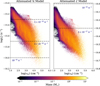Fig. 1 Mass-weighted local CRIR-density 2D-PDF for the attenuated high (ℋ) and low (ℒ) models applied in the dense cloud physical model (see text). The constant CRIR values are denoted as dashed lines.

3.2 Chemical abundances

The abundances of CO, HCO⁺, and N₂H⁺ are plotted as functions of the effective ionization rate, ζ/n_H, for all six ionization models, inFigs. 3–5, respectively. The binned averages, in log-log space, are represented by red lines. The dashed-dotted lines show the abundance profile of the ζ(N)_ℋ model, and dashed lines show the abundance profile of the ζ(N)_ℒ model for comparison. The linear relative error in the average abundance profiles for a particular constant CRIR model in comparison to the ζ(N)_ℋ, ℒ model is calculated by $$\epsilon \left({\chi }_i\right)=\frac{{\chi }_{i,{\zeta }_c}-{\chi }_{i,\zeta {\left(N\right)}_{\mathcal{H},\mathcal{L}}}}{{\chi }_{i,\zeta {\left(N\right)}_{\mathcal{H},\mathcal{L}}}},$$(2) and they are displayed in Fig. A.4. The abundance profiles of CO, HCO⁺, and N₂H⁺ vary significantly as functions of ζ/n_H. In the low-density regime, where ζ/n_H is high, the abundance of CO is greatly diminished. However, it is important to note that in diffuse gas, even in the absence of CRs, the UV radiation field plays a dominant role in driving the chemistry, significantly limiting the formation and survival of CO. The scarcity of CO at low densities has a direct impact on the abundance of HCO⁺, as CO serves as its primary precursor. Consequently, HCO⁺ is extremely rare in this regime, with its abundance relative to CO being as low as 10⁻⁴. Similarly, N₂H⁺ shows limited presence in this region, with its abundance approximately 10⁻⁵ times that of HCO⁺. This limitation is due to the restricted availability of N₂, its precursor, and the intense competition between different ions for reactions.

In the intermediate density regime, where ζ/n_H begins to decrease, CO is shielded from the UV field and starts to increase in abundance as the rates of its formation begin to counterbalance the rates of its destruction. CR attenuation also becomes more effective at protecting CO from CR-induced destruction, allowing it to accumulate. This increase in CO abundance marks a turning point for HCO⁺ formation. In this regime, the destruction of CO by H₃⁺ produces intermediate species that drive the formation of HCO⁺. As a result, the abundance of HCO⁺ rises sharply, reflecting the shift in chemical equilibrium. The increase in HCO⁺ abundance is accompanied by changes in the N₂H⁺ profile. In the early part of the intermediate regime, N₂H⁺ becomes more abundant in regions where CO has not yet accumulated to levels sufficient to act as a significant destroyer of N₂H⁺. However, as CO abundance continues to rise, it reacts with N₂H⁺ (R19), gradually depleting the latter.

At higher densities, the abundance of CO reaches a point where it becomes nearly independent of ζ. In these dense environments, the rate of CO formation surpasses its destruction rate, resulting in saturation at the elemental carbon abundance (χ(CO) ≈ A_C); although this convergence occurs because CO freeze-out onto grain surfaces has not been considered in the network. This underscores the dominant role of CO as the primary reservoir of carbon in these regions. The abundance of HCO⁺ continues to decrease in this regime through reactive collisions with electrons (R12), thus producing CO. A similar characteristic is observed for the abundance profile of N₂H⁺, where CO collisions act as the primary destruction mechanism of N₂H⁺.

The binned average abundance profiles indicate that the ℒ model produces results very similar to a constant ζ_c=5 × 10⁻¹⁷ s⁻¹ model. As we consider higher constant CRIR models, the binned averages gradually shift from the reference line of the ℒ model toward that of the ℋ model. For the physical conditions considered here, the ℒ model shows relatively little attenuation, whereas the ℋ model exhibits factors of five or more in the abundance differences due to attenuation effects.

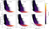Fig. 2 Mass-weighted density-temperature phase plot in semi-logarithmic scale (logarithmic in density). Density increases from left to right. The CR model is annotated in each panel.

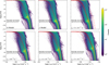Fig. 3 CO abundance profile; χ(CO) versus effective ionization rate, ζ/nH. Density increases from right to left. The CR model is annotated in each panel. The red lines denote the binned averaged abundance profiles in log-log space. The dashed-dotted lines show the ζ(N)ℋ model, and the dashed lines show the ζ(N)ℒ model abundance profile for comparison.

Fig. 4 Same as Fig. 3, but for HCO+ abundance profile. Density increases from right to left.

Fig. 5 Same as Fig. 3, but for N2H+ abundance profile. Density increases from right to left.

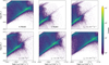Fig. 6 Zoomed-in view (−18.5 ≤ log (ζ/nH) ≤−17.0) and filtered (UV ≤ 1 G0) version of the ${\mathrm{H}}_3^{+}$ abundance profile.

4 Discussion

4.1 Benchmarking ${\mathrm{H}}_3^{+}$ analytic chemistry

${\mathrm{H}}_3^{+}$ plays a critical role in interstellar chemistry, serving as an essential tracer of CR ionization. Due to its relatively simple structure and the fact that its formation and destruction pathways are well understood, ${\mathrm{H}}_3^{+}$ can be used as a reliable probe to determine the CRIRs, especially in diffuse molecular clouds. Its abundance is determined by the ionization of H₂, making it an ideal candidate for analytically calibrating CR flux and ionization rates.

The $\chi \left({\mathrm{H}}_3^{+}\right)-\zeta /n_{\mathrm{H}}$ phase space for our different simulations is shown in Fig. A.1. The abundance profile aligns with the expected dependence on CRIR. In low-density (or high-CRIR environments), a higher ${\mathrm{H}}_3^{+}$ abundance is observed, reflecting the increased ionization activity. As the density increases, the ${\mathrm{H}}_3^{+}$ abundance converges toward a certain upper limit, maintaining a relatively steady value throughout the intermediate-to-high-density regime before dropping down at higher densities. A clear linear trend in the log-log phase space, between the region of −18.5 ≤ log (ζ/n_H) ≤−17.0, is observed. With the expectation that this selected region will serve as a reliable reference for the analytical ${\mathrm{H}}_3^{+}$ calibrators commonly used in the literature to constrain CR-ionization rates, we proceeded to further analyze the region. This analysis aims to validate the applicability of these calibrators under the observed conditions, providing a more accurate assessment of CR effects. A zoomedin view and filtered version of the selected region is displayed in Fig. 6.

Indriolo & McCall (2012) used the ${\mathrm{H}}_3^{+}$ line of sight columndensity measurements to estimate CRIRs in diffuse clouds by comparing observed values with model analytic calibrators. Thus, we aim to test the robustness of these analytic calibrators using our numerical modeling results. The goal is to determine the extent to which the calibrations of ${\mathrm{H}}_3^{+}$ match numerical simulations, providing a deeper understanding of how CRs drive chemistry in different interstellar regions and to what degree the calibrators can capture the CR chemistry. The following expressions of the calibrators are used in Indriolo & McCall (2012): $$\left(\frac{\zeta }{n_{\mathrm{H}}}\right)=k_e{\chi }_e\frac{\chi \left({\mathrm{H}}_3^{+}\right)}{\chi \left({\mathrm{H}}_2\right)},$$(3) $$\begin{array}{rl}& \left(\frac{\zeta }{n_{\mathrm{H}}}\right)\chi \left({\mathrm{H}}_2\right)=\chi \left({\mathrm{H}}_2^{+}\right)[k_3{\chi }_e+k_4\chi (\mathrm{H})+k_2\chi \left({\mathrm{H}}_2\right)],\\ & k_2\chi \left({\mathrm{H}}_2\right)\chi \left({\mathrm{H}}_2^{+}\right)=\chi \left({\mathrm{H}}_3^{+}\right)[k_e{\chi }_e+k_{\mathrm{C}\mathrm{O}}\chi (\mathrm{C}\mathrm{O})+k_9\chi (\mathrm{O})].\end{array}$$(4)

The corresponding rate coefficients are listed in Table 2, where k_e=k₅+k₆ and k_CO=k₇+k₈. Equation (3) uses the simple electron-recombination balance and is denoted as the “first-order calibrator.” Equation (4) employs a more complex approach to the creation and annihilation of ${\mathrm{H}}_3^{+}$, utilizing different recombination chemistry, and it is denoted as the “second-order calibrator.”

The viability of ${\mathrm{H}}_3^{+}$ calibrators, derived from a first-order expression, is assessed through a comparative analysis of the relative error in ${\mathrm{H}}_3^{+}$ abundance between analytical and numerical results. Figure A.2 illustrates the error graphs. The first-order calibrator shows very limited performance in capturing the chemistry. In the intermediate regime, the relative error remains small, usually ≤ 0.5, as most of the data points reside there. But in regions of both low and high density, the relative error becomes significantly larger. Especially at ζ/n_H ≤ 10⁻¹⁸ cm³ s⁻¹, the data are very much scattered. In these regions, the relative error can exceed 1.0, indicating that the first-order calibration struggles to capture the complexity of the chemical interactions. A constant offset of 13% (marked by a dashed black line) is visible in all the models. The limitations of the first-order expression can, in principle, be minimised by including additional reactions, which become relevant at higher ionization rates but are not accounted for in this simplified version; this leads to substantial deviations between the analytical and numerical solutions. Notably, this comparison was performed with data filtered for UV fields below 1 G₀, minimizing the influence of UV radiation.

In contrast, the second-order calibrator incorporates key reactions involving CO and O, which are known to influence ${\mathrm{H}}_3^{+}$ abundance in environments with higher ionization rates. One notable exclusion in Eq. (4) is the reaction between ${\mathrm{H}}_3^{+}$ and carbon (C) atoms; it plays a significant role in the destruction of ${\mathrm{H}}_3^{+}$. Neglecting this interaction can lead to discrepancies between analytical and numerical solutions. To address this limitation, we modified the second-order calibrator by incorporating a more comprehensive chemical network, taking into account total oxygen and carbon chemistry. Specifically, we included R10 and R11 from Table 2, which account for the interactions among ${\mathrm{H}}_3^{+}$, carbon, and oxygen species. This leads to a new coupled analytical expression: $$\begin{array}{rl}& \left(\frac{\zeta }{n_{\mathrm{H}}}\right)\chi \left({\mathrm{H}}_2\right)=\chi \left({\mathrm{H}}_2^{+}\right)[k_3{\chi }_e+k_4\chi (\mathrm{H})+k_2\chi \left({\mathrm{H}}_2\right)],\\ & k_2\chi \left({\mathrm{H}}_2\right)\chi \left({\mathrm{H}}_2^{+}\right)=\chi \left({\mathrm{H}}_3^{+}\right)[k_e{\chi }_e+k_{\mathrm{C}\mathrm{O}}\chi (\mathrm{C}\mathrm{O})+k_{\mathrm{O}}\chi (\mathrm{O})+k_{11}\chi (\mathrm{C})],\end{array}$$(5) where k_O=k₉+k₁₀. This revised expression performs remarkably well, especially from low-to-intermediate-density regions, bringing it close to zero for all the ζ models, as shown in Fig. 7. The modified second-order calibrator reduces the relative error to less than 30%. Again, a constant shift, now of 6.5% is observed throughout the models. Notably, the dense region remains scattered for higher CRIR models, but the error range has been significantly reduced. By integrating a more detailed reaction network, we offer a more accurate and reliable representation of H₃⁺ chemistry across a broader range of ionization rates.

4.2 CRIR calibrators using carbon-cycle species

The χ(HCO⁺)/χ(CO) ratio is a reliable indicator of ionizationdriven chemistry. In dense gas, HCO⁺ forms primarily through the reaction of H₃⁺ (produced via ionization of H₂ by CRs; (R1)–(R2)) with CO (R7). This reaction directly links HCO⁺ formation to the ionization rate. Because HCO⁺ is produced through ${\mathrm{H}}_3^{+}$ interactions with CO, in gas where CO is more abundant, the increased collision rate enhances HCO⁺ production. Thus, without substantial attenuation of the ionization rate, the χ(HCO⁺)/χ(CO) ratio rises with increasing density.

The χ(C⁺)/χ(CO) ratio is also sensitive to ionization, but it reflects the balance between carbon ionization and molecular conversion processes. CRs ionize atomic carbon and other neutral species to form C⁺. At higher ζ, the ionization of neutral carbon is more pronounced alongside the CO destruction caused by He⁺ (R13), leading to an increased abundance of C⁺ relative to CO. In dense and shielded regions where CR attenuation becomes significant, the abundance of C⁺ decreases as carbon is predominantly locked in CO. This makes the χ(C⁺)/χ(CO) ratio a useful tracer for identifying ionization effects, particularly in regions with varying CR penetration. This relationship, however, is complicated by the fact that C⁺ will also be abundant in the envelope of clouds due to UV-driven chemistry, which can influence the overall χ(C⁺)/χ(CO) ratio.

Figures 8 and 9 show χ(HCO⁺)/χ(CO) as a function of ζ/n_e and χ(C⁺)/χ(CO) as a function of ζ/n_H, respectively. The analysis focuses on data filtered under the constraint that the UV-radiation field is below 0.1 G₀. This criterion is applied to isolate dense regions where CRs dominate the chemistry, minimizing the effects of UV-driven photochemistry, which prevails in diffuse, low-density environments. To provide a more comprehensive view, the abundance ratios are mass weighted, emphasizing the dominant processes affecting the bulk of the gas mass rather than the gas volume. This approach accounts for the fact that dense gas contributes significantly to the total mass of molecular clouds but occupies a smaller fraction of the clouds’ volume.

The χ(HCO⁺)/χ(CO) ratio in dense regions exhibits a near-linear behaviour in log−log space, as shown in Fig. 8 with the pink slope. Most of the gas mass resides in this dense regime, which dominates the trend. In the top left portion of the phase space, corresponding to more diffuse regions, the ratio is more scattered and not deterministic, with the total gas mass being <1 M_⊙. In contrast, the χ(C⁺)/χ(CO) ratio shows a much larger spread across the entire phase space. Nevertheless, most of the mass again lies in the dense regime. Between ζ/n_H ∼ 10⁻²⁰ and 10⁻¹⁸, the ratio undergoes a rapid increase as carbon in the diffuse gas is efficiently ionized to C⁺, explaining the sharp transition over this range. This behavior is consistent with the C⁺ abundance profile as a function of n_H depicted in Fig. 7 of Gaches et al. (2022a).

Finally, to understand the observed profile trends, we derived analytical expressions for the χ(HCO⁺)/χ(CO) and χ(C⁺)/χ(CO), based on the probable dominant steady-state formation and destruction pathways of the respective species. These analytical expressions provide a quantitative framework to interpret the trends, linking the observed ratios to the underlying chemical processes in dense molecular gas. The derived expressions are as follows: $$\frac{\chi \left({\mathrm{HCO}}^{+}\right)}{\chi \left(\mathrm{CO}\right)}=\frac{k_7{k}_2{\left[\chi \left({\mathrm{H}}_2\right)\right]}^2}{k_{12}[k_3{\chi }_e+k_2\chi \left({\mathrm{H}}_2\right)][k_e{\chi }_e+k_7\chi \left(\mathrm{CO}\right)]}·\left(\frac{\zeta }{n_e}\right),$$(6) $$\frac{\chi \left({\mathrm{C}}^{+}\right)}{\chi \left(\mathrm{CO}\right)}=\frac{C{k}_{13}\chi \left(\mathrm{He}\right)}{[k_{13}\chi \left(\mathrm{CO}\right)+k_{14}\chi \left({\mathrm{O}}_2\right)][k_{15+gr}{\chi }_e+k_{{\mathrm{C}}^{+}}\chi \left({\mathrm{O}}_2\right)]}·\left(\frac{\zeta }{n_{\mathrm{H}}}\right),$$(7) where $$\mathcal{C}={\alpha }_1^{\mathrm{\prime }}+{\alpha }_2^{\mathrm{\prime }};\{\begin{array}{l}{\alpha }_1^{\mathrm{\prime }}=0.5\\ {\alpha }_2^{\mathrm{\prime }}=0.2/(1.0-0.42)=\mathrm{0.345.}\end{array}$$(8)

The corresponding rate coefficients are listed in Table 2, where k_e = k₅ + k₆, k_C⁺ = k₁₆ + k₁₇, and k_15+gr is the sum of gas-phase electron recombination of C⁺ (R15) and grain assisted recombination, taken from Gong et al. (2017). The ${\alpha }_1^{\text{'}}$ and ${\alpha }_2^{\text{'}}$ (normalized with respect to ζ₀=1.3 × 10⁻¹⁷ s⁻¹) come from the contribution of CRs and CR photons, giving rise to an ζ_eff (see Appendix B.2) for the formation of He⁺ from He. Figures 10 and 11 present the mass-weighted 1:1 comparison plots for the analytical calibrator and the numerically filtered data for the abundance ratios of HCO⁺/CO and C⁺/CO. The dashed black line represents the 1:1 reference line. The χ(HCO⁺)/χ(CO) plot shows a near-linear trend, suggesting that the derived analytical expression effectively captures the chemistry governing this abundance ratio with a constant offset of 0.2 from the 1.1 line. The 0.2 offset is due to our assumption that H₃⁺ is primarily destroyed by collisions with CO. However, 1D steady-state models showed that depending on the density, the contribution of H₃⁺ + CO to the total H₃⁺ destruction can range from 0.4–0.65, with the rest of the contribution being collisions with O and N₂, which are difficult to observe directly. Multiplying k₇ in the denominator by two in Eq. (6), or adding reactions between O or N₂ and H₃⁺ removes this offset. However, both of these species are difficult to measure directly in dense molecular gas. In denser gas, the k_eχe term becomes much less important, so it can be neglected when densities exceed 10³ cm⁻³ without significant error.

In contrast, the χ(C⁺)/χ(CO) plot initially stays parallel with the 1: 1 reference line, but towards the right, a slight deviation is observed, indicating that in those regions, the analytical expression fails to predict the abundance ratio compared to the numerical results. Despite this, the majority of the mass remains aligned with the 1: 1 line, pointing to a broadly consistent trend throughout the models. The observed deviations are likely due to minor side reactions involving neutral C intermediates, which are not integrated in the simplified analytical framework. Notably, the approximation of χ(O₂)=0.5 × χ(CO) ×(χ(O)/χ(C)), where χ(O) and χ(C) are the standard ISM abundances at solar metallicity, is also a good approximation, and plugging it in Eq. (7) gives the results depicted in Fig. A.3. However, we focused on the raw abundance (as it is more transparent) while comparing the analytical and numerical results.

As depicted in Fig. 12, the abundance ratio of N₂H⁺/HCO⁺ as a function of ζ/n_H does not exhibit a clear trend. Interestingly, our results show that the gas-phase production pathways alone can reproduce the N₂H⁺/HCO⁺ abundance ratio from the modeling without explicitly including a dependence on the CRIR. Both ions are formed and destroyed primarily through a tightly coupled set of reactions –formation via ${\mathrm{H}}_3^{+}$ collisions, destruction through dissociative recombination with electrons, and the exchange reaction (R19) linking HCO⁺ and N₂H⁺. These processes operate in a manner such that both species are produced in tandem, and variations in the exchange reaction are largely temperature driven. Since the temperature itself is only indirectly influenced by ζ, the ratio displays little direct sensitivity to the ionization parameter in our gas-phase-only treatment.

The absence of grain-surface chemistry further contributes to the flatness of the N₂H⁺/HCO⁺ ratio. In dense regions, freezeout of species such as CO and subsequent desorption processes – thermal, CR induced, or reactive – strongly alter the abundances of HCO⁺ and N₂H⁺. These grain-mediated processes break the tight gas-phase coupling and introduce additional pathways that reshape the ratio, particularly by suppressing HCO⁺ through CO depletion while enhancing N₂H⁺. Such effects have been demonstrated by Entekhabi et al. (2022), which incorporated CO freeze-out and CR-induced thermal desorption in one-zone infrared dark cloud (IRDC) models and showed that these mechanisms are essential for reproducing observed abundances of CO, HCO⁺, and N₂H⁺. Including grain chemistry in future work will therefore be crucial for capturing the full behavior of the N₂H⁺/HCO⁺ ratio and its true dependence on the ionization environment.

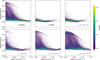Fig. 7 Relative error between numerical abundance profile (3d-pdr) and the modified analytical expressions of ${\mathrm{H}}_3^{+}$ (Eq. (5)). The constant offset of 6.5% is denoted by the dashed black line.

Fig. 8 HCO+ and CO abundance ratio, χ(HCO+)/χ(CO), versus ζ/ne. Density increases from left to right. The CR model is annotated in each panel. The data are filtered under the constraint UV<0.1 G0 and mass weighted. A linear fit (pink line) in log-log space with slope =1 is overlaid.

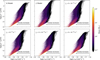Fig. 9 C+ and CO abundance ratio, χ(C+)/χ(CO), as a function of ζ/nH. Density increases from right to left. The CR model is annotated in each panel. The data are filtered under the constraint UV<0.1 G0 and mass weighted.

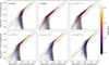Fig. 10 Mass-weighted 1: 1 comparison plots between analytical calibrators and numerical results for the abundance ratio, χ(HCO+)/χ(CO). The CR model is annotated in each panel. The dashed black line represents the 1: 1 reference, and the dashed green line shows the linearity of the data and the relative deviation in linearity among the models. The data are filtered under the constraints UV <0.1 G0 and nH>103 cm−3 for clarity.

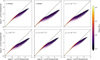Fig. 11 Same as Fig. 10, but for χ(C+)/χ(CO). The data are filtered under the constraints UV <0.1 G0 and nH>103 cm−3 for clarity.

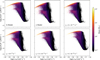Fig. 12 Same as Fig. 9, but for χ(N2H+)/χ(HCO+). Density increases from right to left. The CR model is annotated in each panel. The data are filtered under the constraint UV<0.1 G0 and mass weighted.

4.3 Analytical estimation of the electron fraction

A potential caveat in using all the analytical expressions suggested above is the dependence on the electron fraction, χ_e, which cannot be readily measured observationally and must instead be inferred through indirect methods, such as estimates based on recombination rates or ion-abundance ratios. A common simplification in astrochemical models is to assume that HCO⁺ is a primary carrier of positive charge, often adopting the approximation χ(HCO⁺)/χ_e ∼ 0.5. While this serves as a practical constraint for CRIR estimation, it may not capture the full complexity of ionization processes across different environments. Although analytical expressions for estimating the χ_e have been proposed (Feng et al. 2016; Luo et al. 2024; Latrille et al. 2025), a robust, general estimator valid across a wide density range remains lacking, mainly due to the inclusion of N₂H⁺ as a charge carrier in previous approximations.

Recent work by Pineda et al. (2024), which mapped the NGC 1333 SE region, revealed a smooth χ_e distribution with a typical median value of 10^−6.5. This suggests that the actual χ_e values are significantly higher than the HCO⁺ abundance, highlighting the limitations of the approximation χ_e = 2χ(HCO⁺). While some studies use the alternative approximation χ_e = χ(C⁺), this approach tends to underestimate χ_e in regions where the CRIR is high enough for H⁺ to become the dominant source of electrons (Indriolo & McCall 2012; Indriolo et al. 2012; Indriolo et al. 2015; Bialy & Sternberg 2015).

To address these limitations, we propose a more accurate representation of the electron fraction given by $${\chi }_e=\chi \left({\mathrm{H}}^{+}\right)+\chi \left({\mathrm{C}}^{+}\right)+2\chi \left({\mathrm{HCO}}^{+}\right).$$(9) This formulation provides a better estimate of χ_e, as shown by the one-dimensional model results in Fig. 13. The one-dimensional model uses an A_V−n_H density distribution that reproduces the behaviors seen in three-dimensional simulations, namely exhibiting low (high) density gas at low (high) extinction; see Appendix C, Bisbas et al. (2019), and Gaches (2025). Additionally, it remains within a ± 60% error range in three-dimensional space with −30% in higher density regions, as depicted in Fig. 14. This approach offers a more reliable method for estimating CRIR in astrochemical models, though further refinements are necessary to develop a robust analytical estimator for χ_e.

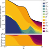Fig. 13 1D AV−nH slab for charge contribution. The top panel displays the abundance of electrons (solid line) and the corresponding analytical expression (dashed line). The colors show cumulative contributions to the ion balance for positive ions, and the bottom panel shows the normalized cumulative contributions with respect to electron abundance.

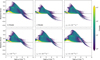Fig. 14 Relative error between numerical electron fraction (3d-pdr) and the analytical electron-fraction expression (Eq. (9)).

5 Conclusions and outlook

Building upon the work of Gaches et al. (2022a), we expanded the previous study by incorporating a more comprehensive chemical network that includes nitrogen chemistry. Additionally, we investigated the impact of CR attenuation, ζ(N), through both the ℋ and ℒ models. Our key findings are as follows:

1. The numerical results successfully reproduce the steady-state analytic ${\mathrm{H}}_3^{+}$ abundances with an error of less than 30%, which is consistent with the hydrogen-electron balance analytical approach used to constrain the CRIR. The revised expression performs remarkably well, particularly from low-to-intermediate-density regions, bringing the error close to zero (see Fig. 7). By incorporating a more detailed reaction network, this approach provides a more accurate and reliable representation of ${\mathrm{H}}_3^{+}$ chemistry across a broader range of ionization conditions;

2. The abundance ratios HCO⁺/CO and C⁺/CO exhibit a highly correlated relationship across all CR models, particularly in dense molecular regions, making them robust tracers of ionization conditions. The numerical results closely align with analytical calibrations, although the deviation from the 1: 1 line in C⁺/CO (see Fig. 11) suggests additional side reactions not fully captured by the simplified chemistry;

3. In contrast, the N₂H⁺/HCO⁺ abundance ratio does not exhibit a clear trend as a function of ζ/n_H, likely due to the absence of grain chemistry in our model. This highlights the significance of surface reactions in determining ion abundances, particularly in the densest cloud environments (n_H>10⁴ cm⁻³);

4. The revised formulation for estimating the χ_e provides an improved estimate compared to an A_V−n_H PDR model and maintains an error margin within ±60% in three-dimensional phase-space. This suggests it may be a more reliable prescription for CRIR in astrochemical models, though further refinements are required to develop a robust analytical estimator.

The low CRIR values inferred in IRDCs by Entekhabi et al. (2022) may themselves be a signature of attenuation processes, further motivating the kind of physically driven modeling approach presented in this work. Future studies need to include grain-surface processes such as CO freeze-out and CR-induced desorption to better reflect the physical conditions of dense regions such as IRDCs, as also emphasized by Entekhabi et al. (2022). These would further enhance the model’s ability to reproduce observed molecular trends in IRDCs and other dense regions of the ISM.

In summary, our results provide a detailed investigation of CR attenuation effects on molecular-ionization chemistry and abundance profiles. The use of a column-density-dependent CRIR prescription significantly improves agreement with observational diagnostics and highlights the limitations of constant-ionization-rate models. Our findings support the need for nonuniform CRIR treatments in dense molecular clouds.

Acknowledgements

The authors thank the anonymous referee for the comments, which improved the clarity of this work. AR acknowledges support from the Chalmers Astrophysics and Space Sciences Summer (CASSUM) research fellowship. BALG is supported by the German Research Foundation (DFG) in the form of an Emmy Noether Research Group – DFG project #542802847 (GA 3170/3-1). JCT acknowledges support from ERC Advanced grant 788828 (MSTAR). The computations were performed on the Dardel/PDC supercomputing facility, enabled by resources provided by the National Academic Infrastructure for Supercomputing in Sweden (NAISS), partially funded by the Swedish Research Council through grant agreement no. 2022-06725 through the allocations NAISS 2024/1-27 and NAISS 2024/6-292. The authors gratefully acknowledge the computing time granted by the Center for Computational Sciences and Simulation (CCSS) of the University of Duisburg-Essen and provided on the supercomputer amplitUDE (DFG project 459398823; grant ID INST 20876/423-1 FUGG) at the Center for Information and Media Services (ZIM).

References

Appendix A Abundance profiles and relative errors

The following figures provide an overview of the key abundance profiles and relative errors discussed in the main text. Figure A.1 shows the ${\mathrm{H}}_3^{+}$ abundance profile, $\chi \left({\mathrm{H}}_3^{+}\right)$, versus the effective ionization rate, ζ/n_H, density increasing from right to left. Figure A.2 presents the relative error between the numerical 3d-pdr abundance profile and the first-order analytical expression of ${\mathrm{H}}_3^{+}$ (Eq. 3 from Indriolo & McCall 2012). Figure A.3 shows the approximate χ(C⁺)/χ(CO) 1:1 phase plot. Figure A.4 displays the linear-relative error in the average abundance profiles for constant CRIR models compared to ζ(N)_ℒ (top) and ζ(N)_ℋ (bottom).

Fig. A.1 Same as Fig. 3 but for the ${\mathrm{H}}_3^{+}$ abundance profile. Density increases from right to left.

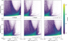Fig. A.2 Relative error between the numerical abundance profile (3d-pdr) and first-order analytical expression of ${\mathrm{H}}_3^{+}$ abundance, calculated using Eq. 3 from Indriolo & McCall (2012). The constant offset of 13% is denoted by the dashed black line.

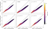Fig. A.3 Same as Fig. 11 but for the approximate abundance of χ(O2). The data is filtered under the constraints: UV <0.1 G0 and nH>103 cm−3 for clarity.

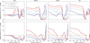Fig. A.4 Linear-relative error in the average abundance profiles for a particular constant CRIR model in comparison to the ζ(N)ℒ (top) and ζ(N)ℋ (bottom) model, calculated using Eq. 2.

Appendix B Derivation of the carbon-cycle calibrators

Appendix B.1 Steady-state derivation of the HCO⁺/CO abundance ratio

We consider the following key ion-molecule reactions in the ISM (reaction and rates no. are same as Table 2): $${\mathrm{H}}_2+\mathrm{C}\mathrm{R}\to {\mathrm{H}}_2^{+}+e^{-}(\zeta )$$(B.1) $${\mathrm{H}}_2^{+}+{\mathrm{H}}_2\to {\mathrm{H}}_3^{+}+\mathrm{H}(k_2)$$(B.2) $${\mathrm{H}}_2^{+}+e^{-}\to \mathrm{H}+\mathrm{H}\left(k_3\right)$$(B.3) $${\mathrm{H}}_3^{+}+e^{-}\to \text{products}(k_5+k_6=k_e)$$(B.4) $${\mathrm{H}}_3^{+}+\mathrm{CO}\to {\mathrm{HCO}}^{+}+{\mathrm{H}}_2\left(k_7\right)$$(B.5) $${\mathrm{HCO}}^{+}+e^{-}\to \mathrm{CO}+\mathrm{H}\left(k_{12}\right).$$(B.6) Under steady-state conditions for each ion:

• (i)

  For ${\mathrm{H}}_2^{+}$: $$\zeta n\left({\mathrm{H}}_2\right)=n\left({\mathrm{H}}_2^{+}\right)[k_{2}n\left({\mathrm{H}}_2\right)+k_3{n}_e]⟹n\left({\mathrm{H}}_2^{+}\right)=\frac{\zeta n\left({\mathrm{H}}_2\right)}{k_{2}n\left({\mathrm{H}}_2\right)+k_3{n}_e}.$$(B.7)

• (ii)

  For ${\mathrm{H}}_3^{+}$: Formation via ${\mathrm{H}}_2^{+}+{\mathrm{H}}_2$ and destruction via CO and e⁻ recombination yield $$k_{2}n\left({\mathrm{H}}_2^{+}\right)n\left({\mathrm{H}}_2\right)=n\left({\mathrm{H}}_3^{+}\right)[k_{7}n\left(\mathrm{CO}\right)+k_e{n}_e]$$(B.8) Substituting $n\left({\mathrm{H}}_2^{+}\right)$ from above gives $$n\left({\mathrm{H}}_3^{+}\right)=\frac{k_2\zeta {\left[n\left({\mathrm{H}}_2\right)\right]}^2}{[k_{2}n\left({\mathrm{H}}_2\right)+k_3{n}_e][k_{7}n\left(\mathrm{CO}\right)+k_e{n}_e]}$$(B.9)

• (iii)

  For HCO⁺: Formation via ${\mathrm{H}}_3^{+}+\mathrm{CO}$ and destruction via dissociative recombination lead to $$k_{7}n\left({\mathrm{H}}_3^{+}\right)n\left(\mathrm{CO}\right)=k_{12}n\left({\mathrm{HCO}}^{+}\right)n_e⟹\frac{n\left({\mathrm{HCO}}^{+}\right)}{n\left(\mathrm{CO}\right)}=\frac{k_{7}n\left({\mathrm{H}}_3^{+}\right)}{k_{12}{n}_e}$$(B.10) Substituting $n\left({\mathrm{H}}_3^{+}\right)$ from Eq. (B.9) gives $$\frac{n\left({\mathrm{HCO}}^{+}\right)}{n\left(\mathrm{CO}\right)}=\frac{k_7{k}_2\zeta {\left[n\left({\mathrm{H}}_2\right)\right]}^2}{k_{12}{n}_e[k_{2}n\left({\mathrm{H}}_2\right)+k_3{n}_e][k_{7}n\left(\mathrm{CO}\right)+k_e{n}_e]}$$(B.11)

• (iv)

  In terms of fractional abundances: Defining χ(i)=n(i)/n_H and χ_e = n_e/n_H, we obtain $$\boxed{{\displaystyle \frac{\chi \left({\mathrm{H}\mathrm{C}\mathrm{O}}^{+}\right)}{\chi (\mathrm{C}\mathrm{O})}=\frac{k_7{k}_2{\left[\chi \left({\mathrm{H}}_2\right)\right]}^2}{k_{12}[k_2\chi \left({\mathrm{H}}_2\right)+k_3{\chi }_e][k_7\chi (\mathrm{C}\mathrm{O})+k_e{\chi }_e]}\cdot \left(\frac{\zeta }{n_e}\right)}}$$(B.12)

Appendix B.2 Steady-state derivation of the C⁺/CO abundance ratio

We consider the following key reactions for helium ionization: $$\mathrm{He}+\mathrm{CRP}\to {\mathrm{He}}^{+}+e^{-}({\zeta }_{\mathrm{CRP}}={\alpha }_1\zeta )$$(B.13) $$\mathrm{H}\mathrm{e}+\text{CRPHOT}\to {\mathrm{H}\mathrm{e}}^{+}+e^{-}({\zeta }_{\text{CRPHOT\hspace{0.17em}}}={\alpha }_2\zeta ).$$(B.14) The ionization of helium is therefore initiated through two distinct pathways: (i) direct ionization by cosmic-ray particles (CRP) and (ii) ionization by secondary cosmic-ray-induced photons (CRPHOT), with rate coefficients α₁ = 6.5 × 10⁻¹⁸ s⁻¹ and α₂ = (1.3 × 10⁻¹⁷) ×(0.2 /[1−0.42]) s⁻¹, respectively.

To express these in normalized form relative to the reference cosmic-ray ionization rate ζ₀=1.3 × 10⁻¹⁷ s⁻¹, we define the dimensionless parameters $${\alpha }_1^{\text{'}}=\frac{{\alpha }_1}{{\zeta }_0},{\alpha }_2^{\text{'}}=\frac{{\alpha }_2}{{\zeta }_0},$$(B.15) yielding ${\alpha }_1^{\text{'}}=0.5$ and ${\alpha }_2^{\text{'}}\approx 0.345$. The total effective ionization rate of helium is then $$\boxed{{\displaystyle {\zeta }_{\mathrm{e}\mathrm{f}\mathrm{f}}=\zeta ({\alpha }_1^{\mathrm{\prime }}+{\alpha }_2^{\mathrm{\prime }})=\zeta \mathcal{C}}},$$(B.16) where ζ is the primary cosmic-ray ionization rate of H₂.

Hence, for the calculation of the steady-state abundance ratio of C⁺/CO, we consider the following key reactions in the gas-phase network: $$\mathrm{H}\mathrm{e}+\mathrm{C}\mathrm{R}\to {\mathrm{H}\mathrm{e}}^{+}+e^{-}(\mathcal{C}\zeta )$$(B.17) $${\mathrm{He}}^{+}+\mathrm{CO}\to {\mathrm{C}}^{+}+\mathrm{O}+\mathrm{He}\left(k_{13}\right)$$(B.18) $${\mathrm{He}}^{+}+{\mathrm{O}}_2\to {\mathrm{O}}^{+}+\mathrm{O}+\mathrm{He}\left(k_{14}\right)$$(B.19) $${\mathrm{C}}^{+}+e^{-}\to \mathrm{C}+hv\left(k_{15}\right)$$(B.20) $${\mathrm{C}}^{+}+{\mathrm{O}}_2\to \text{products}(k_{{\mathrm{C}}^{+}}=k_{16}+k_{17}).$$(B.21) Additionally, including the grain-mediated recombination reactions from Gong et al. (2017), for the reaction C⁺+e⁻+gr → C+gr, we get: $${\alpha }_{\mathrm{g}}={10}^{-14}\frac{C_0}{1+C_1{\Psi }^{C_2}+C_1\Psi C_2-C_5-C_{6}lnT{C}_3{T}^{C_4}},$$ where, $\Psi =1.68{\mathrm{UV}}_{\text{ext}}exp[-{\mathrm{UV}}_{\text{fac}}{A}_{V,\text{eff}}]\frac{\sqrt{T}}{n_e}$ and the constants are, $$C_0=45.58,C_1=6.089\times {10}^{-3},C_2=1.128,C_3=4.331\times {10}^2,C_4=4.845\times {10}^{-2},C_5=0.8120,C_6=1.333\times {10}^{-4},$$ $${\mathrm{UV}}_{\text{ext}}=10G_0,{\mathrm{UV}}_{\text{fac}}=3.02$$ Hence, the Total rate for electron recombination, k_15+gr = k₁₅ + (α_g/χ_e); the division with χ_e is there as a normalization factor, converting the grain-assisted recombination rate from the formulation used by Gong et al. (2017) into a standard two-body rate coefficient compatible with the rest of our chemical network.

Under steady-state conditions for each ion:

• (i)

  For He⁺: $$\mathcal{C}\zeta n(\mathrm{H}\mathrm{e})=n\left({\mathrm{H}\mathrm{e}}^{+}\right)[k_{13}n(\mathrm{C}\mathrm{O})+k_{14}n\left({\mathrm{O}}_2\right)]⟹n\left({\mathrm{H}\mathrm{e}}^{+}\right)=\frac{\mathcal{C}\zeta n(\mathrm{H}\mathrm{e})}{k_{13}n(\mathrm{C}\mathrm{O})+k_{14}n\left({\mathrm{O}}_2\right)}.$$(B.22)

• (ii)

  For C⁺: Formation via He⁺+CO and destruction via gas-phase and grain mediated recombination alongside C⁺+O₂ reactions lead to $$n\left({\mathrm{C}}^{+}\right)(k_{{\mathrm{C}}^{+}}n\left({\mathrm{O}}_2\right)+k_{15+gr}{n}_e)=k_{13}n\left({\mathrm{He}}^{+}\right)n\left(\mathrm{CO}\right)⟹\frac{n\left({\mathrm{C}}^{+}\right)}{n\left(\mathrm{CO}\right)}=\frac{k_{13}n\left({\mathrm{He}}^{+}\right)}{k_{{\mathrm{C}}^{+}}n\left({\mathrm{O}}_2\right)+k_{15+gr}{n}_e}.$$(B.23) Substituting n(He⁺)from Eq. (B.22) gives $$\frac{n\left({\mathrm{C}}^{+}\right)}{n(\mathrm{C}\mathrm{O})}=\frac{k_{13}\mathcal{C}\zeta n(\mathrm{H}\mathrm{e})}{[k_{13}n(\mathrm{C}\mathrm{O})+k_{14}n\left({\mathrm{O}}_2\right)][k_{{\mathrm{C}}^{+}}n\left({\mathrm{O}}_2\right)+k_{15+gr}{n}_e]}.$$(B.24)

• (iii)

  In terms of fractional abundances: Defining χ(i)=n(i)/n_H and χ_e = n_e/n_H, we obtain $$\boxed{{\displaystyle \frac{\chi \left({\mathrm{C}}^{+}\right)}{\chi (\mathrm{C}\mathrm{O})}=\frac{k_{13}\mathcal{C}\chi (\mathrm{H}\mathrm{e})}{[k_{13}\chi (\mathrm{C}\mathrm{O})+k_{14}\chi \left({\mathrm{O}}_2\right)][k_{{\mathrm{C}}^{+}}\chi \left({\mathrm{O}}_2\right)+k_{15+gr}{\chi }_e]}\cdot \left(\frac{\zeta }{n_{\mathrm{H}}}\right)}}.$$(B.25)

Appendix C Description of the chemical network and steady-state benchmarks

We present here a general description of the chemical network that was used in the study and the benchmarks of the network that were performed. The network is a subset of UMIST2012 in size between the reduced networks previously used (33 species) and the full network (>200 species), with 77 species primarily with 4 atoms or fewer with a few exceptions for molecular ions necessary for the desired chemistry (NH₄⁺, H₃CO⁺, C₂H₃, and CH₅⁺). The primary goal of the network was to model the gas-phase chemistry of HCN, HNC, N₂H⁺, NH₃, and light hydrocarbons such as C₂ H. The network was constructed by taking the full-sized network and cutting it down in species and reactions in size until a balance was achieved between performance and accuracy. In practice, this was carried out by removing all species and reactions with molecules with more than four atoms and species bearing atoms beyond H/He/C/N/O. Then, species and reactions were added back in manually as needed for the chemistry. The network was benchmarked against the reduced and full network currently in 3d-pdr by computing a grid of 9 different models, consisting of three FUV fields, G₀ = 1, 10, 100 in units of the Draine field (Draine 1978), and three cosmic-ray ionization rates, ζ=10⁻¹⁷, 10⁻¹⁶, 10⁻¹⁵. The benchmark was performed using the “A_V−n_H” density distribution (Bisbas et al. 2019; Gaches 2025), which reproduces the relation $$A_{V,\text{eff}}=0.05exp[1.6{\left(\frac{n_{\mathrm{H}}}{{\mathrm{cm}}^{-3}}\right)}^{0.12}]\mathrm{mag}$$(C.1) This density distribution has the benefit that it probes realistic regimes with low-density, highly irradiated environments and dense, shielded gas. Since 3d-pdr integrates the chemistry to steady state, the benchmarking is performed under this assumption. We emphasize that this network was developed to best reproduce the behavior of the full gas-phase network in average molecular cloud environments, e.g., n_H<10⁴ cm⁻³, and does not include freeze out at this time. The network will be made available with the next public release of 3d-pdr, or upon request.

Figures C.1, C.2, and C.3 show the results of the steady-state benchmarking of the three different networks, reduced (orange), medium (teal), and full (purple). We find that, when compared to the full network, there is minimal difference for the species of concern. We have also performed this benchmark using constant density slabs in steady-state and similarly find no significant deviations for the species of interest. The network will be made available upon request and in the next major public release of 3d-pdr. Since the networks are benchmarked in steady-state, it cannot be guaranteed that they have the same solution over temporal evolution.

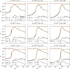Fig. C.1 Abundance of the denoted species, χi, versus visual extinction, AV. Benchmark of the medium-sized chemical network (teal) against the reduced network (orange) and full network (purple), focusing on molecular hydrogen chemistry. The external FUV radiation field, in units of the Draine field (Draine 1978), and cosmic-ray ionization rate are annotated in the subfigure titles.

Fig. C.2 Same as Fig. C.1 but for the carbon cycle, C+/C/CO/HCO+.

Fig. C.3 Same as Fig. C.1 but for HCN, HNC, N2H+, and HCO+.

All Tables

All Figures

	Fig. 1 Mass-weighted local CRIR-density 2D-PDF for the attenuated high (ℋ) and low (ℒ) models applied in the dense cloud physical model (see text). The constant CRIR values are denoted as dashed lines.
In the text

	Fig. 2 Mass-weighted density-temperature phase plot in semi-logarithmic scale (logarithmic in density). Density increases from left to right. The CR model is annotated in each panel.
In the text

	Fig. 3 CO abundance profile; χ(CO) versus effective ionization rate, ζ/nH. Density increases from right to left. The CR model is annotated in each panel. The red lines denote the binned averaged abundance profiles in log-log space. The dashed-dotted lines show the ζ(N)ℋ model, and the dashed lines show the ζ(N)ℒ model abundance profile for comparison.
In the text

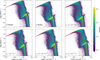	Fig. 4 Same as Fig. 3, but for HCO+ abundance profile. Density increases from right to left.
In the text

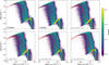	Fig. 5 Same as Fig. 3, but for N2H+ abundance profile. Density increases from right to left.
In the text

	Fig. 6 Zoomed-in view (−18.5 ≤ log (ζ/nH) ≤−17.0) and filtered (UV ≤ 1 G0) version of the ${\mathrm{H}}_3^{+}$ abundance profile.
In the text

	Fig. 7 Relative error between numerical abundance profile (3d-pdr) and the modified analytical expressions of ${\mathrm{H}}_3^{+}$ (Eq. (5)). The constant offset of 6.5% is denoted by the dashed black line.
In the text

	Fig. 8 HCO+ and CO abundance ratio, χ(HCO+)/χ(CO), versus ζ/ne. Density increases from left to right. The CR model is annotated in each panel. The data are filtered under the constraint UV<0.1 G0 and mass weighted. A linear fit (pink line) in log-log space with slope =1 is overlaid.
In the text

	Fig. 9 C+ and CO abundance ratio, χ(C+)/χ(CO), as a function of ζ/nH. Density increases from right to left. The CR model is annotated in each panel. The data are filtered under the constraint UV<0.1 G0 and mass weighted.
In the text

Fig. 10 Mass-weighted 1: 1 comparison plots between analytical calibrators and numerical results for the abundance ratio, χ(HCO+)/χ(CO). The CR model is annotated in each panel. The dashed black line represents the 1: 1 reference, and the dashed green line shows the linearity of the data and the relative deviation in linearity among the models. The data are filtered under the constraints UV <0.1 G0 and nH>103 cm−3 for clarity.

In the text

	Fig. 11 Same as Fig. 10, but for χ(C+)/χ(CO). The data are filtered under the constraints UV <0.1 G0 and nH>103 cm−3 for clarity.
In the text

	Fig. 12 Same as Fig. 9, but for χ(N2H+)/χ(HCO+). Density increases from right to left. The CR model is annotated in each panel. The data are filtered under the constraint UV<0.1 G0 and mass weighted.
In the text

	Fig. 13 1D AV−nH slab for charge contribution. The top panel displays the abundance of electrons (solid line) and the corresponding analytical expression (dashed line). The colors show cumulative contributions to the ion balance for positive ions, and the bottom panel shows the normalized cumulative contributions with respect to electron abundance.
In the text

	Fig. 14 Relative error between numerical electron fraction (3d-pdr) and the analytical electron-fraction expression (Eq. (9)).
In the text

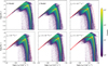	Fig. A.1 Same as Fig. 3 but for the ${\mathrm{H}}_3^{+}$ abundance profile. Density increases from right to left.
In the text

	Fig. A.2 Relative error between the numerical abundance profile (3d-pdr) and first-order analytical expression of ${\mathrm{H}}_3^{+}$ abundance, calculated using Eq. 3 from Indriolo & McCall (2012). The constant offset of 13% is denoted by the dashed black line.
In the text

	Fig. A.3 Same as Fig. 11 but for the approximate abundance of χ(O2). The data is filtered under the constraints: UV <0.1 G0 and nH>103 cm−3 for clarity.
In the text

	Fig. A.4 Linear-relative error in the average abundance profiles for a particular constant CRIR model in comparison to the ζ(N)ℒ (top) and ζ(N)ℋ (bottom) model, calculated using Eq. 2.
In the text

	Fig. C.1 Abundance of the denoted species, χi, versus visual extinction, AV. Benchmark of the medium-sized chemical network (teal) against the reduced network (orange) and full network (purple), focusing on molecular hydrogen chemistry. The external FUV radiation field, in units of the Draine field (Draine 1978), and cosmic-ray ionization rate are annotated in the subfigure titles.
In the text

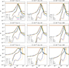	Fig. C.2 Same as Fig. C.1 but for the carbon cycle, C+/C/CO/HCO+.
In the text

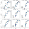	Fig. C.3 Same as Fig. C.1 but for HCN, HNC, N2H+, and HCO+.
In the text

References

- Bayet, E., Williams, D., Hartquist, T., & Viti, S., 2011, MNRAS, 414, 1583 [NASA ADS] [CrossRef] [Google Scholar]
- Bialy, S., & Sternberg, A., 2015, MNRAS, 450, 4424 [NASA ADS] [CrossRef] [Google Scholar]
- Bisbas, T. G., Bell, T. A., Viti, S., Yates, J., & Barlow, M. J., 2012, MNRAS, 427, 2100 [NASA ADS] [CrossRef] [Google Scholar]
- Bisbas, T. G., Papadopoulos, P. P., & Viti, S., 2015, ApJ, 803, 37 [NASA ADS] [CrossRef] [Google Scholar]
- Bisbas, T. G., Schruba, A., & van Dishoeck, E. F., 2019, MNRAS, 485, 3097 [NASA ADS] [Google Scholar]
- Bisbas, T. G., Tan, J. C., & Tanaka, K. E. I., 2021, MNRAS, 502, 2701 [CrossRef] [Google Scholar]
- Bovino, S., Ferrada-Chamorro, S., Lupi, A., Schleicher, D. R. G., & Caselli, P., 2020, MNRAS, 495, L7 [Google Scholar]
- Caselli, P., & Ceccarelli, C., 2012, A&A Rev., 20, 1 [Google Scholar]
- Ceccarelli, C., Caselli, P., Bockelée-Morvan, D., et al. 2014, in Protostars and Planets VI, eds. H. Beuther, R. S. Klessen, C. P. Dullemond, & T. Henning, 859 [Google Scholar]
- Dalgarno, A., 2006, Proc. Natl. Acad. Sci. U.S.A., 103, 12269 [NASA ADS] [CrossRef] [Google Scholar]
- Draine, B. T., 1978, ApJS, 36, 595 [Google Scholar]
- Entekhabi, N., Tan, J. C., Cosentino, G., et al. 2022, A&A, 662, A39 [NASA ADS] [CrossRef] [EDP Sciences] [Google Scholar]
- Feng, S., Beuther, H., Zhang, Q., et al. 2016, A&A, 592, A21 [NASA ADS] [CrossRef] [EDP Sciences] [Google Scholar]
- Gaches, B. A. L., 2025, A&A, 700, L16 [NASA ADS] [CrossRef] [EDP Sciences] [Google Scholar]
- Gaches, B. A. L., & Viti, S., 2025, arXiv e-prints [arXiv:2512.10060] [Google Scholar]
- Gaches, B. A. L., Offner, S. S. R., & Bisbas, T. G., 2019, ApJ, 878, 105 [NASA ADS] [CrossRef] [Google Scholar]
- Gaches, B. A. L., Bisbas, T. G., & Bialy, S. 2022a, A&A, 658, A151 [CrossRef] [EDP Sciences] [Google Scholar]
- Gaches, B. A. L., Bialy, S., Bisbas, T. G., et al. 2022b, A&A, 664, A150 [NASA ADS] [CrossRef] [EDP Sciences] [Google Scholar]
- Gong, M., Ostriker, E. C., & Wolfire, M. G., 2017, ApJ, 843, 38 [NASA ADS] [CrossRef] [Google Scholar]
- Grenier, I. A., Black, J. H., & Strong, A. W., 2015, ARA&A, 53, 199 [Google Scholar]
- Guelin, M., Langer, W. D., Snell, R. L., & Wootten, H. A., 1977, ApJ, 217, L165 [NASA ADS] [CrossRef] [Google Scholar]
- Hsu, C.-J., Tan, J. C., Goodson, M. D., et al. 2021, MNRAS, 502, 1104 [Google Scholar]
- Indriolo, N., & McCall, B. J., 2012, ApJ, 745, 91 [NASA ADS] [CrossRef] [Google Scholar]
- Indriolo, N., & McCall, B. J., 2013, Chem. Soc. Rev., 42, 7763 [Google Scholar]
- Indriolo, N., Geballe, T. R., Oka, T., & McCall, B. J., 2007, ApJ, 671, 1736 [NASA ADS] [CrossRef] [Google Scholar]
- Indriolo, N., Neufeld, D. A., Gerin, M., et al. 2012, ApJ, 758, 83 [NASA ADS] [CrossRef] [Google Scholar]
- Indriolo, N., Neufeld, D. A., Gerin, M., et al. 2015, ApJ, 800, 40 [NASA ADS] [CrossRef] [Google Scholar]
- Ivlev, A. V., Padovani, M., Galli, D., & Caselli, P., 2015, ApJ, 812, 135 [Google Scholar]
- Ivlev, A. V., Dogiel, V. A., Chernyshov, D. O., et al. 2018, ApJ, 855, 23 [NASA ADS] [CrossRef] [Google Scholar]
- Ivlev, A. V., Silsbee, K., Sipilä, O., & Caselli, P., 2019, ApJ, 884, 176 [Google Scholar]
- Kong, S., Caselli, P., Tan, J. C., Wakelam, V., & Sipilä, O., 2015, ApJ, 804, 98 [NASA ADS] [CrossRef] [Google Scholar]
- Kong, S., Tan, J. C., Caselli, P., et al. 2016, ApJ, 821, 94 [NASA ADS] [CrossRef] [Google Scholar]
- Latrille, G., Lupi, A., Bovino, S., et al. 2025, A&A, 699, A126 [NASA ADS] [CrossRef] [EDP Sciences] [Google Scholar]
- Luo, G., Bisbas, T. G., Padovani, M., & Gaches, B. A. L., 2024, A&A, 690, A293 [NASA ADS] [CrossRef] [EDP Sciences] [Google Scholar]
- McCall, B. J., Huneycutt, A., Saykally, R., et al. 2003, Nature, 422, 500 [CrossRef] [Google Scholar]
- McElroy, D., Walsh, C., Markwick, A. J., et al. 2013, A&A, 550, A36 [NASA ADS] [CrossRef] [EDP Sciences] [Google Scholar]
- Morales Ortiz, J. L., Ceccarelli, C., Lis, D. C., et al. 2014, A&A, 563, A127 [NASA ADS] [CrossRef] [EDP Sciences] [Google Scholar]
- Morlino, G., & Gabici, S., 2015, MNRAS, 451, L100 [NASA ADS] [CrossRef] [Google Scholar]
- Mouschovias, T. C., & Spitzer, L., J. 1976, ApJ, 210, 326 [NASA ADS] [CrossRef] [Google Scholar]
- Neufeld, D. A., & Wolfire, M. G., 2017, ApJ, 845, 163 [Google Scholar]
- Neufeld, D. A., Welty, D. E., Ivlev, A. V., et al. 2024, ApJ, 973, 143 [Google Scholar]
- Obolentseva, M., Ivlev, A. V., Silsbee, K., et al. 2024, ApJ, 973, 142 [NASA ADS] [CrossRef] [Google Scholar]
- O’Donoghue, R., Viti, S., Padovani, M., & James, T., 2022, ApJ, 934, 63 [Google Scholar]
- Owen, E. R., On, A. Y. L., Lai, S.-P., & Wu, K. 2021, ApJ, 913, 52 [NASA ADS] [CrossRef] [Google Scholar]
- Padovani, M., & Gaches, B., 2024, in Astrochemical Modeling, eds. S. Bovino, & T. Grassi (Elsevier), 189 [Google Scholar]
- Padovani, M., Galli, D., & Glassgold, A. E., 2009, A&A, 501, 619 [NASA ADS] [CrossRef] [EDP Sciences] [Google Scholar]
- Padovani, M., Ivlev, A. V., Galli, D., & Caselli, P., 2018, A&A, 614, A111 [NASA ADS] [CrossRef] [EDP Sciences] [Google Scholar]
- Padovani, M., Ivlev, A. V., Galli, D., et al. 2020, Space Sci. Rev., 216, 29 [Google Scholar]
- Padovani, M., Bialy, S., Galli, D., et al. 2022, A&A, 658, A189 [NASA ADS] [CrossRef] [EDP Sciences] [Google Scholar]
- Panessa, M., Seifried, D., Walch, S., et al. 2023, MNRAS, 523, 6138 [NASA ADS] [CrossRef] [Google Scholar]
- Phan, V. H. M., Morlino, G., & Gabici, S., 2018, MNRAS, 480, 5167 [NASA ADS] [Google Scholar]
- Pineda, J. E., Sipilä, O., Segura-Cox, D. M., et al. 2024, A&A, 686, A162 [NASA ADS] [CrossRef] [EDP Sciences] [Google Scholar]
- Rathjen, T.-E., Naab, T., Girichidis, P., et al. 2021, MNRAS, 504, 1039 [NASA ADS] [CrossRef] [Google Scholar]
- Redaelli, E., Bovino, S., Lupi, A., et al. 2024, A&A, 685, A67 [NASA ADS] [CrossRef] [EDP Sciences] [Google Scholar]
- Redaelli, E., Sipilä, O., Padovani, M., et al. 2021, A&A, 656, A109 [NASA ADS] [CrossRef] [EDP Sciences] [Google Scholar]
- Rimmer, P. B., Herbst, E., Morata, O., & Roueff, E., 2012, A&A, 537, A7 [NASA ADS] [CrossRef] [EDP Sciences] [Google Scholar]
- Sabatini, G., Bovino, S., Redaelli, E., et al. 2024, A&A, 692, A265 [NASA ADS] [CrossRef] [EDP Sciences] [Google Scholar]
- Schlickeiser, R., 2002, Cosmic Ray Astrophysics (Berlin: Springer) [Google Scholar]
- Schlickeiser, R., Caglar, M., & Lazarian, A., 2016, ApJ, 824, 89 [NASA ADS] [CrossRef] [Google Scholar]
- Silsbee, K., & Ivlev, A. V., 2019, ApJ, 879, 14 [NASA ADS] [CrossRef] [Google Scholar]
- Socci, A., Sabatini, G., Padovani, M., Bovino, S., & Hacar, A., 2024, A&A, 687, A70 [NASA ADS] [CrossRef] [EDP Sciences] [Google Scholar]
- Tielens, A. G., 2005, The Physics and Chemistry of the Interstellar Medium (Cambridge University Press) [Google Scholar]
- Wolfire, M. G., Vallini, L., & Chevance, M., 2022, ARA&A, 60, 247 [Google Scholar]
- Wootten, A., Snell, R., & Glassgold, A., 1979, ApJ, 234, 876 [NASA ADS] [CrossRef] [Google Scholar]
- Wu, B., Tan, J. C., Nakamura, F., et al. 2017, ApJ, 835, 137 [NASA ADS] [CrossRef] [Google Scholar]
3d-pdr can also solve the CR attenuation using a spectrum-resolved solver, but in this work we used the prescribed polynomial function due to memory constraints and the possibility to compare with contemporary studies.