| Issue |
A&A
Volume 708, April 2026
|
|
|---|---|---|
| Article Number | A242 | |
| Number of page(s) | 7 | |
| Section | Extragalactic astronomy | |
| DOI | https://doi.org/10.1051/0004-6361/202556832 | |
| Published online | 08 April 2026 | |
Nitrogen abundances in star-forming galaxies 2.2 Gyr after the Big Bang are not elevated
1
Department of Astronomy, University of Geneva, Chemin Pegasi 51, 1290 Versoix, Switzerland
2
CNRS, IRAP, 14 Avenue E. Belin, 31400 Toulouse, France
3
Bogolyubov Institute for Theoretical Physics, National Academy of Sciences of Ukraine, 14-b Metrolohichna Str., Kyiv 03143, Ukraine
4
Cahill Center for Astronomy and Astrophysics, California Institute of Technology, 1216 East California Boulevard., MS 249-17, Pasadena, CA 91125, USA
5
Department of Physics and Astronomy, University of California, Riverside, 900 University Avenue, Riverside, CA 92521, USA
6
Department of Physics and Astronomy, University of California, Los Angeles, 430 Portola Plaza, Los Angeles, CA 90095, USA
7
Institute of Science and Technology Austria (ISTA), Am Campus 1, 3400 Klosterneuburg, Austria
8
Department of Astronomy, The University of Texas at Austin, Austin, TX 78712, USA
9
Institute for Astronomy, University of Edinburgh, Royal Observatory, Edinburgh EH9 3HJ, UK
10
Center for Astrophysical Sciences, Department of Physics & Astronomy, Johns Hopkins University, Baltimore, MD 21218, USA
11
School of Earth and Space Exploration, Arizona State University, Tempe, AZ 85287, USA
12
Space Telescope Science Institute, 3700 San Martin Dr., Baltimore, MD 21218, USA
13
Waseda Research Institute for Science and Engineering, Faculty of Science and Engineering, Waseda University, 3-4-1 Okubo, Shinjuku, Tokyo 169-8555, Japan
14
Department of Physics, School of Advanced Science and Engineering, Faculty of Science and Engineering, Waseda University, 3-4-1 Okubo, Shinjuku, Tokyo 169-8555, Japan
15
Graduate School of Arts and Sciences, The University of Tokyo, 3-8-1 Komaba, Meguro-ku, Tokyo 153-8902, Japan
16
Cosmic Dawn Center (DAWN), Niels Bohr Institute, University of Copenhagen, Jagtvej 128, København N, DK-2200, Denmark
17
Department of Astronomy, The Oskar Klein Centre, Stockholm University, AlbaNova SE-10691, Stockholm, Sweden
18
INAF – Osservatorio Astronomico di Roma, Via Frascati 33, 00078 Monteporzio Catone, Italy
19
INAF – Osservatorio di Astrofisica e Scienza dello Spazio di Bologna, Via Gobetti 93/3, 40129 Bologna, Italy
20
Department of Astronomy & Astrophysics, The Pennsylvania State University, University Park, PA 16802, USA
21
Institute for Computational & Data Sciences, The Pennsylvania State University, University Park, PA 16802, USA
22
Institute for Gravitation and the Cosmos, The Pennsylvania State University, University Park, PA 16802, USA
★ Corresponding author: This email address is being protected from spambots. You need JavaScript enabled to view it.
Received:
12
August
2025
Accepted:
16
February
2026
Abstract
Using deep, medium-resolution, JWST rest-optical spectra of a sample of typical star-forming galaxies (Lyman-break galaxies and Lyman-α emitters) from the LyC22 survey at z ∼ 3, we determined the nebular abundances of N, O, and Ne relative to H for a subsample of 25 objects with a direct method based on auroral [O III] λ4363 line detections. Our measurements increased the number of accurate N/O determinations at z ∼ 2 − 4 using a homogeneous approach. We found a mean value of log(N/O) = −+0.25−0.21 over a metallicity range of 12 + log(O/H) = 7.56 to 8.44. The observed N/O ratio and scatter are indistinguishable from that observed in low-z galaxies and H II regions over the same metallicity range, thus showing no redshift evolution of N/O for typical galaxies over a significant fraction of cosmic time. We also show that typical z ∼ 3 galaxies have a similar offset in the BPT diagram to galaxies from the low-z Lyman Continuum Survey (LzLCS) when compared to the average of SDSS galaxies, and we demonstrate that this offset is not due to enhanced nitrogen abundances. Our results establish a basis for future studies of the evolution of N and O at higher redshifts.
Key words: galaxies: abundances / galaxies: high-redshift / galaxies: ISM
© The Authors 2026
 Open Access article, published by EDP Sciences, under the terms of the Creative Commons Attribution License (https://creativecommons.org/licenses/by/4.0), which permits unrestricted use, distribution, and reproduction in any medium, provided the original work is properly cited.
This article is published in open access under the Subscribe to Open model. This email address is being protected from spambots. You need JavaScript enabled to view it. to support open access publication.
1. Introduction
The cosmic origin of nitrogen, an element that is abundant in the cosmos and important for life, has been studied for a long time (e.g. Edmunds & Pagel 1978; Henry et al. 2000), and its observed evolution in Milky Way stars, H II regions, and low-redshift galaxies is fairly well understood and reproduced by chemical-evolution models (e.g. Vincenzo & Kobayashi 2018). Recent JWST observations revealed a new category of rare objects showing emission lines of N IV] λ1486 and N III] λ1750 in the rest-UV (hereafter named N-emitters), which are found to show highly supersolar N/O abundance ratios (by factors of ≳2 in several cases) yet subsolar O/H ones (see compilation of Ji et al. 2026), although not exclusively, as the discovery of new N-emitters shows (Morel et al. 2025). The nature of these objects, including the z = 10.6 galaxy GN-z11, the source of enrichment, or other mechanisms leading to a high N/O ratio, are currently a topic of active debate.
To place N-emitters into context, a major question remains, however, concerning the nitrogen abundance and N/O ratio of typical galaxies at high redshift. From stacks of ∼1000 low-resolution (PRISM) spectra taken with NIRSpec/JWST, Hayes et al. (2025) suggested a possible increase of N/O at z > 4 from the UV lines compared to the abundances observed at low redshift. However, the determination of chemical abundances from these spectra is very uncertain. Other studies have used deep, medium-resolution, rest-optical JWST spectra to measure auroral lines for accurate determinations of metallicities (O/H) and the [N II] λ6584 line to then determine the N-abundance. So far, this has been achieved for a small number of galaxies (∼30) spanning a large redshift range (z ∼ 1.8 − 6.3), finding a spread of N/O ratios and only few objects (∼6) with supersolar N/O (Arellano-Córdova et al. 2025a; Scholte et al. 2025; Stiavelli et al. 2025; Marques-Chaves et al. 2025), including lensed galaxies such as RXCJ2248 and the Sunburst arc (Pascale et al. 2023; Topping et al. 2024; Welch et al. 2025; Berg et al. 2025). Another recent study analyzed rest-optical spectra from the MARTA program and other JWST archival data, suggesting that the median N/O abundance ratio of z > 1 galaxies could be elevated by ∼0.18 dex at fixed metallicity (O/H) compared to the average N/O–O/H relations established locally (Cataldi et al. 2025a).
To address these questions and establish the typical N-abundance in “typical” star-forming galaxies (SFGs) at high redshift, we present an analysis of 117 deep JWST spectra of Lyman-break galaxies (LBGs) and Lyman-α emitters (LAEs) at z ∼ 3 drawn from the LyC22 survey (GO 1869, PI: Schaerer), from which we determined accurate chemical abundances of N, O, and Ne relative to H using the direct method for 25 galaxies. We show how their abundance ratios compare with low- and high-redshift galaxies and discuss how these galaxies behave in the BPT diagram (Baldwin et al. 1981) and how the N-abundance affects this diagram.
The structure of our paper is as follows. In Sect. 2, we briefly describe our JWST observations, data reduction, and measurements, as well as comparison samples. The methods adopted to determine elemental abundances are described in Sect. 3. The BPT diagram of the LyC22 sample is shown and discussed in Sect. 4. In Sect. 5, we present the derived abundances and discuss the behavior of N/O. Our main conclusions are summarized in Sect. 6.
2. Observations
The LyC22 survey is a JWST spectroscopic program for testing indirect indicators of Lyman continuum escape, studying the interstellar medium, radiation field, and other properties of known Lyman-continuum emitters and a control sample of z ∼ 3 galaxies, building on the KLCS and LACES surveys (Steidel et al. 2018; Fletcher et al. 2019; Pahl et al. 2021). These surveys mostly included narrow-band-selected Lyα emitters and Lyman-break galaxies at z ∼ 2.5 − 3.5, which represent the main populations of star-forming galaxies at these redshifts (e.g. Shapley 2011). We therefore refer to these galaxies as “typical” star-forming galaxies at this epoch.
Targeting a mixture of both narrow-band-selected Lyα emitters and Lyman-break galaxies at z ∼ 2.5 − 3.5 in the SSA22 and Westphal fields observed by the KLCS and LACES surveys, the final LyC22 observations have provided 117 spectra from three pointings, with a median spectroscopic redshift of  (for all quantities, we quote the median, 16th, and 84th percentiles of the sample). The LyC22 targets have stellar masses of M★ ∼ 108.3 to 1010.7 M⊙ and star-formation rates of SFR ∼ 1−100 M⊙ yr−1, as derived from standard SED fits assuming a constant SFR. More detailed properties of the sample will be described in a subsequent publication.
2.1. JWST NIRSpec observations
The LyC22 sources were observed with NIRSpec in three different micro-shutter assembly (MSA) pointings (two in the SSA22, one in Westphal). Each MSA slitlet consisted of three micro-shutters. We used the medium-resolution grating/filter combinations G140M/F100LP and G235M/F170LP, delivering a spectral resolving power of R ∼ 1000 and continuous wavelength coverage from 0.97 to 3.07 μm. Each source received total on-source integration times of ≃9.2 hours (G140M) and ≃8.8 hours (G235M), which were distributed over 18 individual integrations using the NRSIRS2 readout mode. We reached a 3σ median line-flux sensitivity of ≃2.5 × 10⁻¹⁹ and ≃1.8 × 10⁻¹⁹ erg s−1 cm−2 in the blue and red gratings (for a line width of 300 km s−1).
Data reduction was performed using the official JWST calibration pipeline (v1.13.4) for Level 1 data and the msaexp1 package (v0.7.3; Brammer 2023) for Levels 2 and 3. Processing steps included subtraction of bias and dark current, correction for 1/f noise, and detection and masking of cosmic-ray snowballs. We adopted the calibration reference data system (CRDS) context jwst_1202.pmap to apply flat-field corrections and perform wavelength and flux calibration. The 2D spectra from each slitlet were drizzle-combined, and background subtraction was applied using the standard three-shutter nod pattern. 1D science and error spectra were extracted using the optimal extraction method of Horne (1986) from the rectified G235M 2D spectra, and the same extraction parameters were applied to the G140M data. The error spectra were rescaled upwards to match the observed rms. The 1D spectra were resampled onto a common wavelength grid and flux-matched in the overlapping region (λ ≃ 1.73 − 1.85 μm). Finally, we followed the approach described in Reddy et al. (2023) to determine wavelength-dependent slit losses using a fit of the light profile from the NIRCam F277W images and comparing the fraction of light captured within the slit and extraction apertures as a function of wavelength.
The deep, medium-resolution NIRSpec observations provide a full spectral coverage over ∼2800 − 6800 Å in the rest frame, including the major indicators of LyC escape recently established from studies at low z (cf. Flury et al. 2022a; Jaskot et al. 2024) and numerous other emission lines of interest. Spectra of two LyC22 star-forming galaxies with clear [O III] λ4363 auroral line detections (discussed below) are shown in Fig. 1 for illustration.
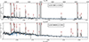 |
Fig. 1. JWST spectra from LyC22 showing object 1005 (top panel, LACES z = 3.676 LAE in SSA22) and 300009 (bottom panel, z = 2.767 LBG in the Westphal field). The blue line shows the adopted fit to the continuum. The main emission and absorption lines are indicated. |
2.2. Emission-line measurements
We modelled the stellar continuum of each LyC22 source using the pPXF software (Cappellari 2017), allowing us to account for underlying stellar absorption, particularly beneath Balmer lines (see Fig. 1). The fits were performed using fsps stellar population-synthesis models (Conroy & Gunn 2010), allowing for ages between 1 Myr and 2.2 Gyr. After continuum subtraction, emission-line fluxes were measured using LiMe (Fernández et al. 2024), fitting Gaussian profiles within a rest-frame spectral window of 20 Å centered on the expected wavelength to the spectra and using tailored continuum windows. Closely spaced emission lines such as Hα and [N II] λλ6550, 6585 were fit simultaneously with multiple Gaussians. We measured a comprehensive set of emission lines from a list of more than 40 features from [Ne IV] λ2423 to [Ar III] λ7751. Finally, emission-line fluxes were corrected for extinction using the Balmer decrement. We used the main Balmer lines (Hα, Hβ, Hγ, and Hδ) and adopted the extinction curve from Cardelli et al. (1989), assuming standard nebular conditions (ne = 100 cm−3 and Te = 104). The median extinction of the LyC22 sources is low: 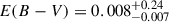 .
.
2.3. Comparison samples
We also compared the LyC22 sources with galaxies from the low-z Lyman Continuum Survey (LzLCS) at z ∼ 0.3 (Flury et al. 2022a,b). This sample includes 66 star-forming galaxies observed with Hubble in the UV and Lyman continuum, which were selected to span a range of UV slopes, SFR surface densities, and [O III] λλ4959,5007/[O II] λλ3727,3729 ratios (Flury et al. 2022b), and 23 compact star-forming galaxies observed earlier by Izotov and collaborators (e.g. Izotov et al. 2016, 2018). The resulting sample includes, for example, galaxies with stellar masses of M★ ∼ 107.3−1010.5 M⊙ and SFR(UV) ∼ 1−100 M⊙ yr−1, and SFR surface densities of log(ΣSFR)∼ − 1 to 2 M⊙ yr−1 kpc−2. Although relatively heterogenous, the low-z comparison sample (89 SFGs) is biased toward low metallicity and more actively star-forming galaxies overall, and it does not represent the full distribution of z ∼ 0 star-forming galaxies from the SDSS.
In terms of stellar mass and SFR, the LzLCS and LyC22 show a strong overlap (see above), although the low-z sample also includes ten objects with masses of M★ ∼ 107 − 108 M⊙, which is below the range covered by LyC22. Further overlaps of these samples are shown below.
Finally, we also compared our results with other JWST observations from the literature, in particular with other studies discussing the nitrogen abundance and N/O in star-forming galaxies, including results from programs such as MARTA, AURORA, EXCELS, and others (Arellano-Córdova et al. 2025a; Sanders et al. 2025; Scholte et al. 2025; Stiavelli et al. 2025; Cataldi et al. 2025a). The properties of the targets of these programs are very diverse, and the selection criteria generally are not very well constrained.
3. Nebular abundance determination
Since accurate abundance determinations require auroral lines, we examined all objects with potential [O III] λ4363 detections. After eliminating the previously identified AGN and following careful visual inspection, this led to a final sample of 25 galaxies with robust [O III] λ4363 detections. We then followed the protocol of Izotov et al. (2006) to determine abundances using the direct method.
Electron densities, measured from the [S II] λλ6717,6731 doublet, are relatively low ( cm−3), and the electron temperatures are not unusual (Te(O III) =
 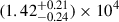 K) for subsolar metallicity star-forming regions. They also agree with those from other studies at z ∼ 1 − 3 using other JWST observations (see e.g. Sanders et al. 2025; Cataldi et al. 2025b).
The electron temperature, Te(O III), was used to obtain the ionic abundances of O2+ and Ne2+; the temperature in the low-ionization region, Te(O II), obtained from the former as described by Izotov et al. (2006), was used to derive the ionic abundance of O+ and N+. For the total oxygen abundance O/H, we used the ionic abundances of O2+/H+ and O+/H+, finding that the former generally dominates in our objects. For N/H, we used the optical [N II] λ6584 lines and the ionization correction factor (ICF) from Izotov et al. (2006); this was similar for Ne/H, for which we used [Ne III] λ3869.
For the LzLCS sample, we derived N/O from the extinction-corrected [N II]/[O II] ratio following Strom et al. (2017), and we took their metallicities (O/H) from the original papers (Flury et al. 2022a,b).
Finally, we also compared our abundance determinations to those using the direct method, but with other prescriptions; for example, for the Te(O II), which is not directly measured, or for the ICF of N/O. In Fig. 2, we compare the N/O abundances derived for the LyC22 using our method to those obtained from the extinction-corrected [N II] λ6584/[O II] λλ3727,3729 line ratio with the prescription from Strom et al. (2017) and the more recently derived fits from Cataldi et al. (2025a), which provided strong line calibrations for N/O using a high-z galaxy sample observed with JWST and an SDSS sample. As Fig. 2 shows, our N/O measurements correlate well with their JWST-based calibration, with an average offset of −0.105 dex. Furthermore, we also see that their SDSS calibration agrees very well with that of Strom et al. (2017), which we used for the LzLCS comparison sample, thus further justifying the use of this relation for our low-z sources. Further discussions and comparisons of methods to determine N/O abundances from the optical-line ratios are discussed in Cataldi et al. (2025a). In short, we conclude that our standard methodology is in good agreement with other studies, with the caveat of a systematic shift in the N/O abundance of ∼ − 0.1 dex compared to the N/O strong line calibration of Cataldi et al. (2025a), which does not, however, affect our conclusions (see below).
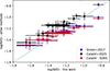 |
Fig. 2. Comparison of N/O abundances derived following the direct method and the assumptions described in this work (x-axis) with those adopting the strong line calibrations of Cataldi et al. (2025a) based on JWST samples (in black; applicable for z > 1) and an SDSS sample (red, applicable at low z), and the calibration from Strom et al. (2017) (blue). All strong line calibrations used the extinction-corrected line ratio of [N II] λ6584/[O II] λλ3727,3729. |
4. BPT diagram of galaxies at z ∼ 3
In Fig. 3, we show the position of the LyC22 sources in one of the classical emission-line (so-called BPT) diagnostic diagrams from Baldwin et al. (1981), together with the “maximum starburst” line from Kewley et al. (2001) and an empirical AGN/star-formation threshold from Kauffmann et al. (2003) established for z ∼ 0 galaxies from the SDSS. Based on this diagram, we robustly identified four LyC22 sources as AGNs, which is also confirmed by their broad hydrogen emission lines. The remainder of our objects were found below the discrimination line of Kewley et al. (2001), and the majority were also below the line from Kauffmann et al. (2003); therefore, they are compatible with photoionization by massive stars. Interestingly, these SF-AGN separations established for z ∼ 0 galaxies are also sufficient to describe the envelope of our z ∼ 3 galaxies, and they do not require shifted separation lines for z ∼ 3, as proposed by several existing studies (e.g. Kewley et al. 2013a,b).
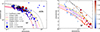 |
Fig. 3. Left: Classical emission-line diagnostic diagram showing the galaxies from the LyC22 sample (blue and red symbols). LyC22 objects with significant [O III] λ4363 detections are surrounded by a black square. LyC22 galaxies with log(N/O) > − 1.2 are shown in red. We only show objects where the involved emission lines are detected at ≥3σ. Typical uncertainties are comparable to the size of the symbols and are hence not plotted. The maximum starburst line from Kewley et al. (2001) (dotted) and the empirical AGN/star-formation threshold from Kauffmann et al. (2003) established for z ∼ 0 (dash-dotted) are also shown. Average relations for z ∼ 2.3 galaxies from Steidel et al. (2014), Shapley et al. (2015) are shown by orange and magenta lines; the average relation of SDSS galaxies from Kewley et al. (2013a) is shown by the red line. Observations from the LzLCS at z ∼ 0.3 are shown by small gray squares. Right: Zoomed-in view of part of the BPT diagram showing all LyC22 sources with color-coded N/O abundances (in log(N/O)); computed from [N II]/[O II]. |
The LyC22 SFGs are in good agreement with the average relations established earlier for z ∼ 2.3 galaxies with Keck observations (Steidel et al. 2014; Shapley et al. 2015). This confirms, for the first time with a large sample at z ∼ 3, the offset of high-z SFGs found previously for z ∼ 2.3 from the average relation of SDSS galaxies, as illustrated by the z ∼ 0 line from Kewley et al. (2013a). Benefiting from accurate abundances for a subset of our galaxies, we also find that galaxies with higher-than-average N/O ratios have systematically higher [N II]/Hα ratios at a given [O III]/Hβ, as shown by the red squares in Fig. 3 (left panel). Indeed, as shown in the right panel, galaxies with increasing N/O abundances are shifted to higher [N II]/Hα ratios at a given [O III]/Hβ, as expected from simple nebular physics, and also observed in SDSS samples (Masters et al. 2016).
We also compared the LyC22 sources with the low-z Lyman Continuum Survey (LzLCS) at z ∼ 0.3 in Fig. 3. They followed very similar sequences in this BPT diagram, thus showing similar excitation properties for the LyC22 and LzLCS samples. Furthermore, since the inferred N/O abundances (see below) are also comparable between these z ∼ 0 and z ∼ 3 samples and not significantly enhanced, this implies that other causes explain the offset in the BPT diagram between the overall z ∼ 0 population and z ∼ 2 − 3 SFGs. For example, Steidel et al. (2016) and Strom et al. (2017) concluded that a harder ionizing spectrum at fixed O/H, due to iron-poor stellar populations, is the most likely explanation for the offset. Alternatively, Masters et al. (2016) have shown that low-z galaxies with higher SFR surface densities are shifted toward the locus of z ∼ 2 − 3 galaxies, which is also reflected in the shift between the overall (average) SDSS population and the LzLCS z ∼ 0.3 by selection (see above). The two explanations could in fact be consistent, since alpha enhancements (increased O/Fe) are equivalent to Fe deficiencies at fixed O/H and are found to increase with increasing specific SFR (sSFR), which also correlates with ΣSFR (e.g. Masters et al. 2016; Flury et al. 2022a).
5. Nitrogen and oxygen abundances in star-forming galaxies at z ∼ 3 and beyond
5.1. Normal nitrogen and oxygen abundances at z ∼ 3
The N/O ratios and metallicities (O/H) of our sample are shown in Fig. 4. O/H ranges from 12 + log(O/H) = 7.56 to 8.44 (with a median of 7.93), the lowest metallicity thus being ∼7% solar (Asplund et al. 2009). With  , the observed N/O ratios of the LyC22 sample are thus clearly subsolar, and both the average N/O ratio and the observed scatter broadly agree with those found in low-z star-forming galaxies and H II regions at the same metallicity, as also shown in this figure. For metallicities of 12 + log(O/H) < 8.45 comparable to LyC22, the Izotov et al. (2023) sample shown here has log(N/O) = − 1.33 ± 0.21, and the LzLCS log(N/O) = − 1.22 ± 0.18.
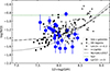 |
Fig. 4. Derived abundance ratio N/O from rest-optical lines of the LyC22 galaxies (blue circles) and low-z samples as a function of O/H. The low-z star-forming galaxies and H II regions from the compilation of Izotov et al. (2023) and the LzLCS are shown by small black and gray symbols, respectively. Dash-dotted and dotted lines show the average trend observed in low-z star-forming galaxies, as parametrized by Vila-Costas & Edmunds (1993) and Nicholls et al. (2017), respectively. The dotted green line shows the solar value. |
We do not consider that the apparent trend of decreasing N/O with increasing O/H is significant2. Comparable galaxies are also found at low z, and the number of objects at 12 + log(O/H)≲7.8 is quite limited. Our sample does not show a correlation of N/O with density either, which, according to Arellano-Córdova et al. (2025b), could explain the observed scatter of N/O. The scatter in the N/O–O/H relation is well known and can in principle be explained in terms of different timescales over which nitrogen and oxygen are released into the ISM (see e.g. Pérez-Montero & Contini 2009; Berg et al. 2019), different star formation histories (e.g. Henry et al. 2000), or other processes, although no dominant mechanism has been identified (see e.g. discussions in Arellano-Córdova et al. 2025b; Cataldi et al. 2025b). However, it has been shown that at a given metallicity, N/O does not correlate with stellar mass (e.g. Masters et al. 2016; Arellano-Córdova et al. 2025b).
In any case, our main empirical finding is that typical star-forming galaxies at z ∼ 3 have essentially the same N/O ratio (and scatter) at a given O/H as galaxies and H II regions at low redshift. With 25 new measurements, our sample increases the number of known galaxies at z ∼ 2 − 4 with accurate N/O measurements from JWST using the same method as here (direct method and optical [N II] lines). This result is also corroborated by the recent study of Cataldi et al. (2025b), which added other data. We also examined the neon abundance ratio, finding 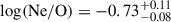 , which is also in good agreement with low-redshift star-forming galaxies (e.g., Guseva et al. 2011).
5.2. The notion of the average N/O ratio at low metallicity increasing beyond z > 4
To examine if at higher redshift (z ≳ 4) the average N/O ratio increases and deviates from the average relation observed at z ∼ 0 − 3, as suggested, for example, by Hayes et al. (2025) and Cataldi et al. (2025a), we show in Fig. 5 the difference Δ(log(N/O)) = log(N/O)−log(N/O)VCE between the derived N/O ratio and the value expected from the relation of Vila-Costas & Edmunds (1993) at the observed O/H. For comparison, we show samples with available abundances determined from JWST spectra using the direct (Te) method and N/O ratios derived from the rest-optical lines, i.e., using the same methodology as our study. This also includes three objects at z ∼ 2.2 − 2.4 studied by Sanders et al. (2023) and Welch et al. (2025), and the lensed N-emitter at z = 6.1 identified by Topping et al. (2024).
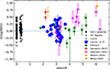 |
Fig. 5. Excess Δ(log(N/O)) of N/O with respect to the local N/O–O/H relation from Vila-Costas & Edmunds (1993) as a function of redshift for galaxies with abundances from the direct method and N/O from rest-optical lines. Low-z star-forming galaxies and H II regions, LzLCS and LyC22 samples are shown with the same symbols as in Fig. 4. Other N/O measurements from the rest-optical lines, obtained primarily from JWST spectra, are shown at z ∼ 2.2 (red symbols, from Sanders et al. 2023), for the EXCELS sample (green stars; Arellano-Córdova et al. 2025a; Scholte et al. 2025), from Stiavelli et al. (2025, magenta), the Sunburst arc at z = 2.4 (orange; Welch et al. 2025), and for the z = 6.1 lensed galaxy (orange) from Topping et al. (2024), with measurements from rest-optical lines by Berg et al. (2025). The two orange symbols indicate objects known to also show UV-emission lines of nitrogen. |
As shown in Fig. 5, N/O also shows a large dispersion at z ≳ 4, and the average N/O ratio is somewhat enhanced with respect to the “local” N/O–O/H relation, although the current samples with accurate abundances are still small. Qualitatively, the same is also found if we use, for example, the more recent local N/O–O/H relation determined by Cataldi et al. (2025a). Clearly, a few individual objects with significant N/O excess measured from the optical lines exist, both at z ∼ 4 − 6 and at z ∼ 2.2, such as the well-studied Sunburst arc (Pascale et al. 2023; Welch et al. 2025) and others. Determining how high and how significant the excess of the average N/O ratio is, and how this evolves at z ≳ 4, requires accurate abundance determinations in larger samples of typical galaxies at high-z, which is are largely lacking at present.
In this context, it is also interesting to compare our findings with those from studies of rare galaxies showing nitrogen lines (N IV] λ1486 or N III] λ1750) in the UV domain, which we refer to as N-emitters. Fig. 5 shows two such objects, the Sunburst arc at z = 2.4 and RXCJ2248-ID3 at z = 6.1 shown in orange (with an excess Δ(log(N/O)) ∼ 0.7 − 0.9), which both also have a high N/O ratio according to the optical-line ratios. To the best of our knowledge, none of the other z > 2 galaxies plotted in Fig. 5 show reported N-lines in the UV. This is in part due to the absence of rest-UV spectra of these objects, and to the non-detection of these lines. For the z ∼ 2 − 3 galaxies including the LyC22 targets, in particular, deep, ground-based rest-UV spectra have also not shown any detections of the N IV] λ1486 or N III] λ1750 lines, which is in agreement with earlier studies; this shows that these lines are generally not present in UV spectra of z ∼ 2 − 3 star-forming galaxies, and they are only very rarely found individually or in stacks of extreme objects (e.g. Christensen et al. 2012; Le Fèvre et al. 2019). Our finding of a “normal” N/O ratio in “typical” z ∼ 3 galaxies is fully consistent with this picture, where only very few objects show a strong excess in N/O at these redshifts. According to the recent works of Morel et al. (2025) and Schaerer et al. (2025), the fraction of star-forming galaxies showing UV nitrogen lines is fN ∼ (1 − 3)×10−3 at z ∼ 3; this is too low to show up and affect samples such as those studied here. Whether the observed increase of fN with redshift is compatible with and sufficient to explain the possible increase of the average N/O ratio at z ≳ 4 discussed here remains to be examined.
6. Conclusions
We present the first JWST spectra from the LyC22 survey, observing known Lyman-continuum emitters and a control sample at z ∼ 3, selected primarily from earlier LyC studies with the HST and Keck (Steidel et al. 2018; Fletcher et al. 2019; Pahl et al. 2021), which targeted a representative sample of LAEs and LBGs. Using LyC22 spectra with robust detections of the [O III] λ4363 auroral line, we determined accurate chemical abundances of N, O, and Ne relative to H for a subset of 25 star-forming galaxies from their rest-optical emission lines. Their metallicities range between 12 + log(O/H)∼7.5 and ∼8.4, and they all show subsolar N/O abundance ratios,  , which is in agreement with the observed N/O abundances of low-z galaxies and H II regions at the same metallicity. From our data and other existing JWST measurements, we therefore conclude that typical star-forming galaxies (LAEs, LBGs) at z ∼ 3 are not enriched in nitrogen compared to their low-redshift counterparts at a given metallicity’s O/H. Statistics for larger samples and establishing the distribution of N, O, and other elemental abundances, in particular at z ≳ 4, will be of great interest for our understanding of the early chemical evolution of galaxies and the nature of rare N-emitters discovered by the JWST.
Our spectra show that the LyC22 sample closely resembles those of other z ∼ 2 samples in the [N II]/Hα BPT diagram, confirming earlier findings of an offset between SFGs at these redshifts and the average of SDSS galaxies (Steidel et al. 2014; Shapley et al. 2015). From our abundance determinations, we found that galaxies with higher N/O ratios show stronger [N II]/Hα emission, as expected. However, our results imply that observed shifts in the BPT are not due to enhanced N-abundances, as suggested by some earlier studies (e.g. Shapley et al. 2015; Masters et al. 2016). Populations with similar offsets also exist at low-z (e.g., the LzLCS sample), and their offset could be due to higher SFR surface densities or a harder ionizing spectrum at fixed O/H (cf. Masters et al. 2016; Steidel et al. 2016).
Acknowledgments
Y.I., N.G., R.M.-C., and D.S. acknowledge support from project No. 224866 carried out in the framework of the Joint Call “Ukrainian-Swiss Joint Research Projects: Call for Proposals 2023”. This work is based in part on observations made with the NASA/ESA/CSA James Webb Space Telescope. The data were obtained from the Mikulski Archive for Space Telescopes at the Space Telescope Science Institute, which is operated by the Association of Universities for Research in Astronomy, Inc., under NASA contract NAS 5-03127 for JWST. These observations are associated with program # 1869. Support for program # 1869 was provided by NASA through a grant from the Space Telescope Science Institute, which is operated by the Association of Universities for Research in Astronomy, Inc., under NASA contract NAS 5-03127. The data used are publicly available at the Mikulski Archive for Space Telescope (MAST), and can be accessed at https://dx.doi.org/10.17909/x6d5-vd44.
References
- Arellano-Córdova, K. Z., Cullen, F., Carnall, A. C., et al. 2025a, MNRAS, 540, 2991 [Google Scholar]
- Arellano-Córdova, K. Z., Berg, D. A., Mingozzi, M., et al. 2025b, MNRAS, 544, 1588 [Google Scholar]
- Asplund, M., Grevesse, N., Sauval, A. J., & Scott, P. 2009, ARA&A, 47, 481 [NASA ADS] [CrossRef] [Google Scholar]
- Baldwin, J. A., Phillips, M. M., & Terlevich, R. 1981, PASP, 93, 5 [Google Scholar]
- Berg, D. A., Erb, D. K., Henry, R. B. C., Skillman, E. D., & McQuinn, K. B. W. 2019, ApJ, 874, 93 [NASA ADS] [CrossRef] [Google Scholar]
- Berg, D. A., Naidu, R. P., Chisholm, J., et al. 2025, ArXiv e-prints [arXiv:2511.13591] [Google Scholar]
- Brammer, G. 2023, https://doi.org/10.5281/zenodo.7299500 [Google Scholar]
- Cappellari, M. 2017, MNRAS, 466, 798 [Google Scholar]
- Cardelli, J. A., Clayton, G. C., & Mathis, J. S. 1989, ApJ, 345, 245 [Google Scholar]
- Cataldi, E., Belfiore, F., Curti, M., et al. 2025a, A&A, submitted [arXiv:2512.07955] [Google Scholar]
- Cataldi, E., Belfiore, F., Curti, M., et al. 2025b, A&A, 703, A208 [NASA ADS] [CrossRef] [EDP Sciences] [Google Scholar]
- Christensen, L., Richard, J., Hjorth, J., et al. 2012, MNRAS, 427, 1953 [Google Scholar]
- Conroy, C., & Gunn, J. E. 2010, Astrophysics Source Code Library [record ascl:1010.043] [Google Scholar]
- Edmunds, M. G., & Pagel, B. E. J. 1978, MNRAS, 185, 77P [NASA ADS] [CrossRef] [Google Scholar]
- Fernández, V., Amorín, R., Firpo, V., & Morisset, C. 2024, A&A, 688, A69 [NASA ADS] [CrossRef] [EDP Sciences] [Google Scholar]
- Fletcher, T. J., Tang, M., Robertson, B. E., et al. 2019, ApJ, 878, 87 [Google Scholar]
- Flury, S. R., Jaskot, A. E., Ferguson, H. C., et al. 2022a, ApJ, 930, 126 [NASA ADS] [CrossRef] [Google Scholar]
- Flury, S. R., Jaskot, A. E., Ferguson, H. C., et al. 2022b, ApJS, 260, 1 [NASA ADS] [CrossRef] [Google Scholar]
- Guseva, N. G., Izotov, Y. I., Stasińska, G., et al. 2011, A&A, 529, A149 [NASA ADS] [CrossRef] [EDP Sciences] [Google Scholar]
- Hayes, M. J., Saldana-Lopez, A., Citro, A., et al. 2025, ApJ, 982, 14 [Google Scholar]
- Henry, R. B. C., Edmunds, M. G., & Köppen, J. 2000, ApJ, 541, 660 [NASA ADS] [CrossRef] [Google Scholar]
- Horne, K. 1986, PASP, 98, 609 [Google Scholar]
- Izotov, Y. I., Stasińska, G., Meynet, G., Guseva, N. G., & Thuan, T. X. 2006, A&A, 448, 955 [CrossRef] [EDP Sciences] [Google Scholar]
- Izotov, Y. I., Orlitová, I., Schaerer, D., et al. 2016, Nature, 529, 178 [Google Scholar]
- Izotov, Y. I., Worseck, G., Schaerer, D., et al. 2018, MNRAS, 478, 4851 [Google Scholar]
- Izotov, Y. I., Schaerer, D., Worseck, G., et al. 2023, MNRAS, 522, 1228 [NASA ADS] [CrossRef] [Google Scholar]
- Jaskot, A. E., Silveyra, A. C., Plantinga, A., et al. 2024, ApJ, 972, 92 [NASA ADS] [CrossRef] [Google Scholar]
- Ji, X., Belokurov, V., Maiolino, R., et al. 2026, MNRAS, 545, staf2110 [Google Scholar]
- Kauffmann, G., Heckman, T. M., White, S. D. M., et al. 2003, MNRAS, 341, 33 [Google Scholar]
- Kewley, L. J., Heisler, C. A., Dopita, M. A., & Lumsden, S. 2001, ApJS, 132, 37 [Google Scholar]
- Kewley, L. J., Maier, C., Yabe, K., et al. 2013a, ApJ, 774, L10 [Google Scholar]
- Kewley, L. J., Dopita, M. A., Leitherer, C., et al. 2013b, ApJ, 774, 100 [NASA ADS] [CrossRef] [Google Scholar]
- Le Fèvre, O., Lemaux, B. C., Nakajima, K., et al. 2019, A&A, 625, A51 [NASA ADS] [CrossRef] [EDP Sciences] [Google Scholar]
- Marques-Chaves, R., Schaerer, D., Dessauges-Zavadsky, M., et al. 2025, A&A, submitted [arXiv:2510.12411] [Google Scholar]
- Masters, D., Faisst, A., & Capak, P. 2016, ApJ, 828, 18 [NASA ADS] [CrossRef] [Google Scholar]
- Morel, I., Schaerer, D., Marques-Chaves, R., et al. 2025, A&A, submitted [arXiv:2511.20484] [Google Scholar]
- Nicholls, D. C., Sutherland, R. S., Dopita, M. A., Kewley, L. J., & Groves, B. A. 2017, MNRAS, 466, 4403 [Google Scholar]
- Pahl, A. J., Shapley, A., Steidel, C. C., Chen, Y., & Reddy, N. A. 2021, MNRAS, 505, 2447 [NASA ADS] [CrossRef] [Google Scholar]
- Pascale, M., Dai, L., McKee, C. F., & Tsang, B. T. H. 2023, ApJ, 957, 77 [NASA ADS] [CrossRef] [Google Scholar]
- Pérez-Montero, E., & Contini, T. 2009, MNRAS, 398, 949 [CrossRef] [Google Scholar]
- Reddy, N. A., Topping, M. W., Sanders, R. L., Shapley, A. E., & Brammer, G. 2023, ApJ, 948, 83 [NASA ADS] [CrossRef] [Google Scholar]
- Sanders, R. L., Shapley, A. E., Clarke, L., et al. 2023, ApJ, 943, 75 [Google Scholar]
- Sanders, R. L., Shapley, A. E., Topping, M. W., et al. 2025, ArXiv e-prints [arXiv:2508.10099] [Google Scholar]
- Schaerer, D., Marques-Chaves, R., Atek, H., et al. 2025, A&A, submitted [arXiv:2512.16549] [Google Scholar]
- Scholte, D., Cullen, F., Carnall, A. C., et al. 2025, MNRAS, 540, 1800 [Google Scholar]
- Shapley, A. E. 2011, ARA&A, 49, 525 [NASA ADS] [CrossRef] [Google Scholar]
- Shapley, A. E., Reddy, N. A., Kriek, M., et al. 2015, ApJ, 801, 88 [NASA ADS] [CrossRef] [Google Scholar]
- Steidel, C. C., Rudie, G. C., Strom, A. L., et al. 2014, ApJ, 795, 165 [Google Scholar]
- Steidel, C. C., Strom, A. L., Pettini, M., et al. 2016, ApJ, 826, 159 [NASA ADS] [CrossRef] [Google Scholar]
- Steidel, C. C., Bogosavljević, M., Shapley, A. E., et al. 2018, ApJ, 869, 123 [Google Scholar]
- Stiavelli, M., Morishita, T., Chiaberge, M., et al. 2025, ApJ, 981, 136 [Google Scholar]
- Strom, A. L., Steidel, C. C., Rudie, G. C., et al. 2017, ApJ, 836, 164 [NASA ADS] [CrossRef] [Google Scholar]
- Topping, M. W., Stark, D. P., Senchyna, P., et al. 2024, MNRAS, 529, 3301 [NASA ADS] [CrossRef] [Google Scholar]
- Vila-Costas, M. B., & Edmunds, M. G. 1993, MNRAS, 265, 199 [NASA ADS] [CrossRef] [Google Scholar]
- Vincenzo, F., & Kobayashi, C. 2018, MNRAS, 478, 155 [NASA ADS] [CrossRef] [Google Scholar]
- Welch, B., Rivera-Thorsen, T. E., Rigby, J. R., et al. 2025, ApJ, 980, 33 [Google Scholar]
Both Spearmann and Kendall tests yield comparable values of p = 0.02.
All Figures
|
Fig. 1. JWST spectra from LyC22 showing object 1005 (top panel, LACES z = 3.676 LAE in SSA22) and 300009 (bottom panel, z = 2.767 LBG in the Westphal field). The blue line shows the adopted fit to the continuum. The main emission and absorption lines are indicated. |
| In the text | |
|
Fig. 2. Comparison of N/O abundances derived following the direct method and the assumptions described in this work (x-axis) with those adopting the strong line calibrations of Cataldi et al. (2025a) based on JWST samples (in black; applicable for z > 1) and an SDSS sample (red, applicable at low z), and the calibration from Strom et al. (2017) (blue). All strong line calibrations used the extinction-corrected line ratio of [N II] λ6584/[O II] λλ3727,3729. |
| In the text | |
|
Fig. 3. Left: Classical emission-line diagnostic diagram showing the galaxies from the LyC22 sample (blue and red symbols). LyC22 objects with significant [O III] λ4363 detections are surrounded by a black square. LyC22 galaxies with log(N/O) > − 1.2 are shown in red. We only show objects where the involved emission lines are detected at ≥3σ. Typical uncertainties are comparable to the size of the symbols and are hence not plotted. The maximum starburst line from Kewley et al. (2001) (dotted) and the empirical AGN/star-formation threshold from Kauffmann et al. (2003) established for z ∼ 0 (dash-dotted) are also shown. Average relations for z ∼ 2.3 galaxies from Steidel et al. (2014), Shapley et al. (2015) are shown by orange and magenta lines; the average relation of SDSS galaxies from Kewley et al. (2013a) is shown by the red line. Observations from the LzLCS at z ∼ 0.3 are shown by small gray squares. Right: Zoomed-in view of part of the BPT diagram showing all LyC22 sources with color-coded N/O abundances (in log(N/O)); computed from [N II]/[O II]. |
| In the text | |
|
Fig. 4. Derived abundance ratio N/O from rest-optical lines of the LyC22 galaxies (blue circles) and low-z samples as a function of O/H. The low-z star-forming galaxies and H II regions from the compilation of Izotov et al. (2023) and the LzLCS are shown by small black and gray symbols, respectively. Dash-dotted and dotted lines show the average trend observed in low-z star-forming galaxies, as parametrized by Vila-Costas & Edmunds (1993) and Nicholls et al. (2017), respectively. The dotted green line shows the solar value. |
| In the text | |
|
Fig. 5. Excess Δ(log(N/O)) of N/O with respect to the local N/O–O/H relation from Vila-Costas & Edmunds (1993) as a function of redshift for galaxies with abundances from the direct method and N/O from rest-optical lines. Low-z star-forming galaxies and H II regions, LzLCS and LyC22 samples are shown with the same symbols as in Fig. 4. Other N/O measurements from the rest-optical lines, obtained primarily from JWST spectra, are shown at z ∼ 2.2 (red symbols, from Sanders et al. 2023), for the EXCELS sample (green stars; Arellano-Córdova et al. 2025a; Scholte et al. 2025), from Stiavelli et al. (2025, magenta), the Sunburst arc at z = 2.4 (orange; Welch et al. 2025), and for the z = 6.1 lensed galaxy (orange) from Topping et al. (2024), with measurements from rest-optical lines by Berg et al. (2025). The two orange symbols indicate objects known to also show UV-emission lines of nitrogen. |
| In the text | |
Current usage metrics show cumulative count of Article Views (full-text article views including HTML views, PDF and ePub downloads, according to the available data) and Abstracts Views on Vision4Press platform.
Data correspond to usage on the plateform after 2015. The current usage metrics is available 48-96 hours after online publication and is updated daily on week days.
Initial download of the metrics may take a while.