| Issue |
A&A
Volume 708, April 2026
|
|
|---|---|---|
| Article Number | A164 | |
| Number of page(s) | 30 | |
| Section | Extragalactic astronomy | |
| DOI | https://doi.org/10.1051/0004-6361/202557286 | |
| Published online | 08 April 2026 | |
Euclid preparation
LXXXVIII. 3D reconstruction of the cosmic web with Euclid Deep spectroscopic samples
1
Université de Strasbourg, CNRS, Observatoire astronomique de Strasbourg, UMR 7550, 67000 Strasbourg, France
2
Institut d’Astrophysique de Paris, UMR 7095, CNRS, and Sorbonne Université, 98 bis boulevard Arago, 75014 Paris, France
3
Department of Physics and Astronomy, University of Waterloo, Waterloo, Ontario N2L 3G1, Canada
4
Waterloo Centre for Astrophysics, University of Waterloo, Waterloo, Ontario N2L 3G1, Canada
5
Institute of Physics, Laboratory of Astrophysics, Ecole Polytechnique Fédérale de Lausanne (EPFL), Observatoire de Sauverny, 1290 Versoix, Switzerland
6
School of Physics and Astronomy, University of Nottingham, University Park, Nottingham NG7 2RD, UK
7
Max Planck Institute for Extraterrestrial Physics, Giessenbachstr. 1, 85748 Garching, Germany
8
Institut de Recherche en Informatique de Toulouse (IRIT), Université de Toulouse, CNRS, Toulouse INP, UT3, 31062 Toulouse, France
9
Laboratoire MCD, Centre de Biologie Intégrative (CBI), Université de Toulouse, CNRS, UT3, 31062 Toulouse, France
10
Kyung Hee University, Dept. of Astronomy & Space Science, Yongin-shi, Gyeonggi-do 17104, Republic of Korea
11
INAF-Osservatorio Astronomico di Trieste, Via G. B. Tiepolo 11, 34143 Trieste, Italy
12
Institut d’Astrophysique de Paris, 98bis Boulevard Arago, 75014 Paris, France
13
Dipartimento di Fisica “G. Occhialini”, Università degli Studi di Milano Bicocca, Piazza della Scienza 3, 20126 Milano, Italy
14
INAF-Istituto di Astrofisica e Planetologia Spaziali, via del Fosso del Cavaliere, 100, 00100 Roma, Italy
15
Univ. Lille, CNRS, Centrale Lille, UMR 9189 CRIStAL, 59000 Lille, France
16
Université Paris-Saclay, CNRS, Institut d’astrophysique spatiale, 91405 Orsay, France
17
INAF-Osservatorio di Astrofisica e Scienza dello Spazio di Bologna, Via Piero Gobetti 93/3, 40129 Bologna, Italy
18
IFPU, Institute for Fundamental Physics of the Universe, via Beirut 2, 34151 Trieste, Italy
19
Institute of Physics, Laboratory for Galaxy Evolution, Ecole Polytechnique Fédérale de Lausanne, Observatoire de Sauverny, CH-1290 Versoix, Switzerland
20
Department of Astronomy, University of Geneva, ch. d’Ecogia 16, 1290 Versoix, Switzerland
21
Université Côte d’Azur, Observatoire de la Côte d’Azur, CNRS, Laboratoire Lagrange, Bd de l’Observatoire, CS 34229, 06304 Nice cedex 4, France
22
Department of Physics and Astronomy, University of the Western Cape, Bellville, Cape Town 7535, South Africa
23
School of Mathematics and Physics, University of Surrey, Guildford, Surrey GU2 7XH, UK
24
INAF-Osservatorio Astronomico di Brera, Via Brera 28, 20122 Milano, Italy
25
INFN, Sezione di Trieste, Via Valerio 2, 34127 Trieste TS, Italy
26
SISSA, International School for Advanced Studies, Via Bonomea 265, 34136 Trieste TS, Italy
27
Dipartimento di Fisica e Astronomia, Università di Bologna, Via Gobetti 93/2, 40129 Bologna, Italy
28
INFN-Sezione di Bologna, Viale Berti Pichat 6/2, 40127 Bologna, Italy
29
Dipartimento di Fisica, Università di Genova, Via Dodecaneso 33, 16146 Genova, Italy
30
INFN-Sezione di Genova, Via Dodecaneso 33, 16146 Genova, Italy
31
Department of Physics “E. Pancini”, University Federico II, Via Cinthia 6, 80126 Napoli, Italy
32
INAF-Osservatorio Astronomico di Capodimonte, Via Moiariello 16, 80131 Napoli, Italy
33
Instituto de Astrofísica e Ciências do Espaço, Universidade do Porto, CAUP, Rua das Estrelas, PT4150-762 Porto, Portugal
34
Faculdade de Ciências da Universidade do Porto, Rua do Campo de Alegre, 4150-007 Porto, Portugal
35
European Southern Observatory, Karl-Schwarzschild-Str. 2, 85748 Garching, Germany
36
Dipartimento di Fisica, Università degli Studi di Torino, Via P. Giuria 1, 10125 Torino, Italy
37
INFN-Sezione di Torino, Via P. Giuria 1, 10125 Torino, Italy
38
INAF-Osservatorio Astrofisico di Torino, Via Osservatorio 20, 10025 Pino Torinese (TO), Italy
39
European Space Agency/ESTEC, Keplerlaan 1, 2201 AZ, Noordwijk, The Netherlands
40
Institute Lorentz, Leiden University, Niels Bohrweg 2, 2333 CA, Leiden, The Netherlands
41
Leiden Observatory, Leiden University, Einsteinweg 55, 2333 CC, Leiden, The Netherlands
42
INAF-IASF Milano, Via Alfonso Corti 12, 20133 Milano, Italy
43
Centro de Investigaciones Energéticas, Medioambientales y Tecnológicas (CIEMAT), Avenida Complutense 40, 28040 Madrid, Spain
44
Port d’Informació Científica, Campus UAB, C. Albareda s/n, 08193 Bellaterra (Barcelona), Spain
45
Institut d’Estudis Espacials de Catalunya (IEEC), Edifici RDIT, Campus UPC, 08860 Castelldefels, Barcelona, Spain
46
Institute of Space Sciences (ICE, CSIC), Campus UAB, Carrer de Can Magrans, s/n, 08193 Barcelona, Spain
47
Institute for Theoretical Particle Physics and Cosmology (TTK), RWTH Aachen University, 52056 Aachen, Germany
48
INAF-Osservatorio Astronomico di Roma, Via Frascati 33, 00078 Monteporzio Catone, Italy
49
INFN section of Naples, Via Cinthia 6, 80126 Napoli, Italy
50
Institute for Astronomy, University of Hawaii, 2680 Woodlawn Drive, Honolulu, HI 96822, USA
51
Dipartimento di Fisica e Astronomia “Augusto Righi” – Alma Mater Studiorum Università di Bologna, Viale Berti Pichat 6/2, 40127 Bologna, Italy
52
Instituto de Astrofísica de Canarias, Vía Láctea, 38205 La Laguna, Tenerife, Spain
53
Institute for Astronomy, University of Edinburgh, Royal Observatory, Blackford Hill, Edinburgh EH9 3HJ, UK
54
Jodrell Bank Centre for Astrophysics, Department of Physics and Astronomy, University of Manchester, Oxford Road, Manchester M13 9PL, UK
55
European Space Agency/ESRIN, Largo Galileo Galilei 1, 00044 Frascati, Roma, Italy
56
ESAC/ESA, Camino Bajo del Castillo, s/n., Urb. Villafranca del Castillo, 28692 Villanueva de la Cañada, Madrid, Spain
57
Université Claude Bernard Lyon 1, CNRS/IN2P3, IP2I Lyon, UMR 5822, Villeurbanne F-69100, France
58
Institut de Ciències del Cosmos (ICCUB), Universitat de Barcelona (IEEC-UB), Martí i Franquès 1, 08028 Barcelona, Spain
59
Institució Catalana de Recerca i Estudis Avançats (ICREA), Passeig de Lluís Companys 23, 08010 Barcelona, Spain
60
UCB Lyon 1, CNRS/IN2P3, IUF, IP2I Lyon, 4 rue Enrico Fermi, 69622 Villeurbanne, France
61
Departamento de Física, Faculdade de Ciências, Universidade de Lisboa, Edifício C8, Campo Grande, PT1749-016 Lisboa, Portugal
62
Instituto de Astrofísica e Ciências do Espaço, Faculdade de Ciências, Universidade de Lisboa, Campo Grande, 1749-016 Lisboa, Portugal
63
Aix-Marseille Université, CNRS, CNES, LAM, Marseille, France
64
INFN-Padova, Via Marzolo 8, 35131 Padova, Italy
65
Aix-Marseille Université, CNRS/IN2P3, CPPM, Marseille, France
66
INFN-Bologna, Via Irnerio 46, 40126 Bologna, Italy
67
Universitäts-Sternwarte München, Fakultät für Physik, Ludwig-Maximilians-Universität München, Scheinerstrasse 1, 81679 München, Germany
68
INAF-Osservatorio Astronomico di Padova, Via dell’Osservatorio 5, 35122 Padova, Italy
69
Institute of Theoretical Astrophysics, University of Oslo, P.O. Box 1029 Blindern 0315 Oslo, Norway
70
Jet Propulsion Laboratory, California Institute of Technology, 4800 Oak Grove Drive, Pasadena, CA 91109, USA
71
Felix Hormuth Engineering, Goethestr. 17, 69181 Leimen, Germany
72
Technical University of Denmark, Elektrovej 327, 2800 Kgs, Lyngby, Denmark
73
Cosmic Dawn Center (DAWN), Denmark
74
Max-Planck-Institut für Astronomie, Königstuhl 17, 69117 Heidelberg, Germany
75
NASA Goddard Space Flight Center, Greenbelt, MD 20771, USA
76
Department of Physics and Astronomy, University College London, Gower Street, London WC1E 6BT, UK
77
Department of Physics and Helsinki Institute of Physics, Gustaf Hällströmin katu 2, University of Helsinki, 00014 Helsinki, Finland
78
Université Paris-Saclay, Université Paris Cité, CEA, CNRS, AIM, 91191 Gif-sur-Yvette, France
79
Université de Genève, Département de Physique Théorique and Centre for Astroparticle Physics, 24 quai Ernest-Ansermet, CH-1211 Genève 4, Switzerland
80
Department of Physics, P.O. Box 64, University of Helsinki, 00014 Helsinki, Finland
81
Helsinki Institute of Physics, Gustaf Hällströmin katu 2, University of Helsinki, 00014 Helsinki, Finland
82
Laboratoire d’etude de l’Univers et des phenomenes eXtremes, Observatoire de Paris, Université PSL, Sorbonne Université, CNRS, 92190 Meudon, France
83
SKAO, Jodrell Bank, Lower Withington, Macclesfield SK11 9FT, United Kingdom
84
Centre de Calcul de l’IN2P3/CNRS, 21 avenue Pierre de Coubertin, 69627 Villeurbanne Cedex, France
85
Dipartimento di Fisica “Aldo Pontremoli”, Università degli Studi di Milano, Via Celoria 16, 20133 Milano, Italy
86
INFN-Sezione di Milano, Via Celoria 16, 20133 Milano, Italy
87
University of Applied Sciences and Arts of Northwestern Switzerland, School of Computer Science, 5210 Windisch, Switzerland
88
Universität Bonn, Argelander-Institut für Astronomie, Auf dem Hügel 71, 53121 Bonn, Germany
89
INFN-Sezione di Roma, Piazzale Aldo Moro, 2 – c/o Dipartimento di Fisica, Edificio G. Marconi, 00185 Roma, Italy
90
Dipartimento di Fisica e Astronomia “Augusto Righi” – Alma Mater Studiorum Università di Bologna, via Piero Gobetti 93/2, 40129 Bologna, Italy
91
Department of Physics, Institute for Computational Cosmology, Durham University, South Road, Durham DH1 3LE, UK
92
Université Paris Cité, CNRS, Astroparticule et Cosmologie, 75013 Paris, France
93
CNRS-UCB International Research Laboratory, Centre Pierre Binétruy, IRL2007, CPB-IN2P3 Berkeley, USA
94
Telespazio UK S.L. for European Space Agency (ESA), Camino bajo del Castillo, s/n, Urbanizacion Villafranca del Castillo, Villanueva de la Cañada, 28692 Madrid, Spain
95
Institut de Física d’Altes Energies (IFAE), The Barcelona Institute of Science and Technology, Campus UAB, 08193 Bellaterra (Barcelona), Spain
96
DARK, Niels Bohr Institute, University of Copenhagen, Jagtvej 155, 2200 Copenhagen, Denmark
97
Perimeter Institute for Theoretical Physics, Waterloo, Ontario N2L 2Y5, Canada
98
Space Science Data Center, Italian Space Agency, via del Politecnico snc, 00133 Roma, Italy
99
Centre National d’Etudes Spatiales – Centre spatial de Toulouse, 18 avenue Edouard Belin, 31401 Toulouse Cedex 9, France
100
Institute of Space Science, Str. Atomistilor, nr. 409 Măgurele, Ilfov 077125, Romania
101
Consejo Superior de Investigaciones Cientificas, Calle Serrano 117, 28006 Madrid, Spain
102
Universidad de La Laguna, Departamento de Astrofísica, 38206 La Laguna, Tenerife, Spain
103
Dipartimento di Fisica e Astronomia “G. Galilei”, Università di Padova, Via Marzolo 8, 35131 Padova, Italy
104
Institut für Theoretische Physik, University of Heidelberg, Philosophenweg 16, 69120 Heidelberg, Germany
105
Institut de Recherche en Astrophysique et Planétologie (IRAP), Université de Toulouse, CNRS, UPS, CNES, 14 Av. Edouard Belin, 31400 Toulouse, France
106
Université St Joseph; Faculty of Sciences, Beirut, Lebanon
107
Departamento de Física, FCFM, Universidad de Chile, Blanco Encalada 2008, Santiago, Chile
108
Universität Innsbruck, Institut für Astro- und Teilchenphysik, Technikerstr. 25/8, 6020 Innsbruck, Austria
109
Satlantis, University Science Park, Sede Bld 48940, Leioa-Bilbao, Spain
110
Infrared Processing and Analysis Center, California Institute of Technology, Pasadena, CA 91125, USA
111
Instituto de Astrofísica e Ciências do Espaço, Faculdade de Ciências, Universidade de Lisboa, Tapada da Ajuda, 1349-018 Lisboa, Portugal
112
Cosmic Dawn Center (DAWN)
113
Niels Bohr Institute, University of Copenhagen, Jagtvej 128, 2200 Copenhagen, Denmark
114
Universidad Politécnica de Cartagena, Departamento de Electrónica y Tecnología de Computadoras, Plaza del Hospital 1, 30202 Cartagena, Spain
115
Kapteyn Astronomical Institute, University of Groningen, PO Box 800, 9700 AV, Groningen, The Netherlands
116
Dipartimento di Fisica e Scienze della Terra, Università degli Studi di Ferrara, Via Giuseppe Saragat 1, 44122 Ferrara, Italy
117
Istituto Nazionale di Fisica Nucleare, Sezione di Ferrara, Via Giuseppe Saragat 1, 44122 Ferrara, Italy
118
INAF, Istituto di Radioastronomia, Via Piero Gobetti 101, 40129 Bologna, Italy
119
Astronomical Observatory of the Autonomous Region of the Aosta Valley (OAVdA), Loc. Lignan 39, I-11020 Nus (Aosta Valley), Italy
120
Department of Physics, Oxford University, Keble Road, Oxford OX1 3RH, UK
121
Aurora Technology for European Space Agency (ESA), Camino bajo del Castillo, s/n, Urbanizacion Villafranca del Castillo, Villanueva de la Cañada, 28692 Madrid, Spain
122
Department of Mathematics and Physics E. De Giorgi, University of Salento, Via per Arnesano, CP-I93, 73100 Lecce, Italy
123
INFN, Sezione di Lecce, Via per Arnesano, CP-193, 73100 Lecce, Italy
124
INAF-Sezione di Lecce, c/o Dipartimento Matematica e Fisica, Via per Arnesano, 73100 Lecce, Italy
125
INAF – Osservatorio Astronomico di Brera, via Emilio Bianchi 46, 23807 Merate, Italy
126
INAF-Osservatorio Astronomico di Brera, Via Brera 28, 20122 Milano, Italy, and INFN-Sezione di Genova, Via Dodecaneso 33, 16146 Genova, Italy
127
ICL, Junia, Université Catholique de Lille, LITL, 59000 Lille, France
128
ICSC – Centro Nazionale di Ricerca in High Performance Computing, Big Data e Quantum Computing, Via Magnanelli 2 Bologna, Italy
129
Instituto de Física Teórica UAM-CSIC, Campus de Cantoblanco, 28049 Madrid, Spain
130
CERCA/ISO, Department of Physics, Case Western Reserve University, 10900 Euclid Avenue, Cleveland, OH 44106, USA
131
Technical University of Munich, TUM School of Natural Sciences, Physics Department, James-Franck-Str. 1, 85748 Garching, Germany
132
Max-Planck-Institut für Astrophysik, Karl-Schwarzschild-Str. 1, 85748 Garching, Germany
133
Laboratoire Univers et Théorie, Observatoire de Paris, Université PSL, Université Paris Cité, CNRS, 92190 Meudon, France
134
Departamento de Física Fundamental. Universidad de Salamanca, Plaza de la Merced s/n, 37008 Salamanca, Spain
135
Instituto de Astrofísica de Canarias (IAC); Departamento de Astrofísica, Universidad de La Laguna (ULL), 38200 La Laguna, Tenerife, Spain
136
Center for Data-Driven Discovery, Kavli IPMU (WPI), UTIAS, The University of Tokyo, Kashiwa, Chiba 277-8583, Japan
137
Ludwig-Maximilians-University, Schellingstrasse 4, 80799 Munich, Germany
138
Max-Planck-Institut für Physik, Boltzmannstr. 8, 85748 Garching, Germany
139
Dipartimento di Fisica – Sezione di Astronomia, Università di Trieste, Via Tiepolo 11, 34131 Trieste, Italy
140
California Institute of Technology, 1200 E California Blvd, Pasadena, CA 91125, USA
141
University of California, Los Angeles, CA 90095-1562, USA
142
Department of Physics & Astronomy, University of California Irvine, Irvine, CA 92697, USA
143
Departamento Física Aplicada, Universidad Politécnica de Cartagena, Campus Muralla del Mar, 30202 Cartagena, Murcia, Spain
144
Instituto de Física de Cantabria, Edificio Juan Jordá, Avenida de los Castros, 39005 Santander, Spain
145
Observatorio Nacional, Rua General Jose Cristino, 77-Bairro Imperial de Sao Cristovao, Rio de Janeiro, 20921-400, Brazil
146
Institute of Cosmology and Gravitation, University of Portsmouth, Portsmouth PO1 3FX, UK
147
Department of Computer Science, Aalto University, PO Box 15400 Espoo FI-00 076, Finland
148
Instituto de Astrofísica de Canarias, c/ Via Lactea s/n, La Laguna 38200, Spain. Departamento de Astrofísica de la Universidad de La Laguna, Avda. Francisco Sanchez, La Laguna, 38200, Spain
149
Ruhr University Bochum, Faculty of Physics and Astronomy, Astronomical Institute (AIRUB), German Centre for Cosmological Lensing (GCCL), 44780 Bochum, Germany
150
Department of Physics and Astronomy, Vesilinnantie 5, University of Turku, 20014 Turku, Finland
151
Serco for European Space Agency (ESA), Camino bajo del Castillo, s/n, Urbanizacion Villafranca del Castillo, Villanueva de la Cañada, 28692 Madrid, Spain
152
ARC Centre of Excellence for Dark Matter Particle Physics, Melbourne, Australia
153
Centre for Astrophysics & Supercomputing, Swinburne University of Technology, Hawthorn, Victoria 3122, Australia
154
DAMTP, Centre for Mathematical Sciences, Wilberforce Road, Cambridge CB3 0WA, UK
155
Kavli Institute for Cosmology Cambridge, Madingley Road, Cambridge CB3 0HA, UK
156
Department of Astrophysics, University of Zurich, Winterthurerstrasse 190, 8057 Zurich, Switzerland
157
Department of Physics, Centre for Extragalactic Astronomy, Durham University, South Road, Durham DH1 3LE, UK
158
IRFU, CEA, Université Paris-Saclay, 91191 Gif-sur-Yvette Cedex, France
159
Oskar Klein Centre for Cosmoparticle Physics, Department of Physics, Stockholm University, Stockholm SE-106 91, Sweden
160
Astrophysics Group, Blackett Laboratory, Imperial College London, London SW7 2AZ, UK
161
Univ. Grenoble Alpes, CNRS, Grenoble INP, LPSC-IN2P3, 53, Avenue des Martyrs, 38000 Grenoble, France
162
INAF-Osservatorio Astrofisico di Arcetri, Largo E. Fermi 5, 50125 Firenze, Italy
163
Dipartimento di Fisica, Sapienza Università di Roma, Piazzale Aldo Moro 2, 00185 Roma, Italy
164
Centro de Astrofísica da Universidade do Porto, Rua das Estrelas, 4150-762 Porto, Portugal
165
HE Space for European Space Agency (ESA), Camino bajo del Castillo, s/n, Urbanizacion Villafranca del Castillo, Villanueva de la Cañada, 28692 Madrid, Spain
166
Theoretical astrophysics, Department of Physics and Astronomy, Uppsala University, Box 516, 751 37 Uppsala, Sweden
167
Mathematical Institute, University of Leiden, Einsteinweg 55, 2333 CA, Leiden, The Netherlands
168
Institute of Astronomy, University of Cambridge, Madingley Road, Cambridge CB3 0HA, UK
169
Department of Astrophysical Sciences, Peyton Hall, Princeton University, Princeton, NJ 08544, USA
170
Space physics and astronomy research unit, University of Oulu, Pentti Kaiteran katu 1, FI-90014 Oulu, Finland
171
Center for Computational Astrophysics, Flatiron Institute, 162 5th Avenue, 10010 New York, NY, USA
★ Corresponding author: This email address is being protected from spambots. You need JavaScript enabled to view it.
Received:
17
September
2025
Accepted:
8
January
2026
Abstract
The ongoing Euclid mission is aimed at measuring spectroscopic redshifts for approximately two million galaxies using the Hα line emission detected in near-infrared slitless spectroscopic data from the Euclid Deep Fields, leveraging both the red and blue grisms. These measurements will reach a flux limit of 5 × 10⁻¹⁷ erg cm−2 s−1 in the redshift range 0.4 < z < 1.8, paving the way to numerous scientific investigations involving galaxy evolution, extending well beyond the mission’s core objectives. The achieved Hα luminosity depth will lead to a sufficiently high sampling, enabling the reconstruction of the large-scale galaxy environment. Here, we assess the quality of the reconstruction of the galaxy cosmic web environment with the expected spectroscopic dataset in Euclid Deep Fields. The analysis was carried out on the Flagship and GAEA galaxy mock catalogues. The quality of the reconstruction was first evaluated using simple geometrical and topological statistics measured on the cosmic web network; namely, the length of filaments, the area of walls, the volume of voids, and its connectivity and multiplicity. We then quantified how accurately gradients in galaxy properties can be recovered, with respect to the distance from filaments. As expected, the small-scale redshift-space distortions, such as Fingers of God (FoG) effects, have a strong impact on filament lengths and connectivity; however, they can be mitigated by compressing galaxy groups identified with an anisotropic group finder prior to a skeleton extraction. The cosmic web reconstruction is biased when relying solely on Hα emitters. This limitation can be mitigated by applying stellar mass weighting during the cosmic web reconstruction. However, this approach introduces non-trivial biases that need to be accounted for when comparing to theoretical predictions. Redshift uncertainties pose the greatest challenge in recovering the expected dependence of galaxy properties, although the well-established stellar mass transverse gradients towards filaments can still be observed to a lesser extent.
Key words: galaxies: evolution – cosmology: observations – large-scale structure of Universe
© The Authors 2026
 Open Access article, published by EDP Sciences, under the terms of the Creative Commons Attribution License (https://creativecommons.org/licenses/by/4.0), which permits unrestricted use, distribution, and reproduction in any medium, provided the original work is properly cited.
This article is published in open access under the Subscribe to Open model. This email address is being protected from spambots. You need JavaScript enabled to view it. to support open access publication.
1. Introduction
Since the first observations in the late 1970s, which revealed the existence of coherent patterns on scales larger than those of galaxy clusters, mapping the large-scale structure of the Universe has become possible thanks to large galaxy redshift surveys. Early observations of the nearby Universe have uncovered complex structures of interconnected superclusters (e.g. Davis et al. 1982) and enabled unexpected discoveries of the first large cosmic voids (e.g. Kirshner et al. 1981), providing a preliminary hint that the spatial distribution of galaxies is highly inhomogeneous. It was quickly confirmed that this is a general feature of the large-scale distribution of galaxies, once observations from surveys covering wider areas on the sky started to become available. Beginning with the first redshift slices of the Center of Astrophysics redshift survey (CfA, de Lapparent et al. 1986), the progressively increasing depth and coverage offered by the next generations of surveys such as Las Campanas Redshift Survey (LCRS, Shectman et al. 1996), 2dF Galaxy Redshift Survey (2dFGRS, Colless et al. 2001), Sloan Digital Sky Survey (SDSS, York et al. 2000; Abazajian et al. 2009, for DR7), 6dF Galaxy Survey (6dFGS, Jones et al. 2004, 2009), and Galaxy and Mass Assembly (GAMA, Driver et al. 2011) have allowed us to map the large-scale structure of the nearby Universe (z ≲ 0.3) in unprecedented detail. These surveys have revealed a cosmic landscape where galaxies are distributed within high-density peaks, intermediate-density filaments, and walls, enclosing low-density, nearly empty voids. This view has been extended up to z ≃ 1 by the VIMOS Public Extragalactic Redshift Survey (VIPERS, Guzzo et al. 2014), which encompasses a volume and galaxy sampling density comparable to those of spectroscopic surveys of the local Universe. Further improvement, in terms of significantly increased galaxy number density and depth compared to any of these surveys in the comparable redshift range, will be achieved by the ongoing Dark Energy Spectroscopic Instrument (DESI; DESI Collaboration 2016) collaboration, which has already collected high-confidence spectroscopic redshifts (McCullough et al. 2024) for more than ten million galaxies (DESI Collaboration 2025).
Mapping the large-scale structure in three dimensions at even higher redshifts (z ≳ 1) is currently impossible with existing spectroscopic surveys, due to their rapidly decreasing completeness and sampling number density. For the time being, the density field at high redshifts is observationally accessible only through the tomographic reconstruction using the Lyman-α forest absorption of light from bright background sources, such as quasars, typically at z ∼ 2.5 − 3 (e.g. Lee & White 2016; Ravoux et al. 2020). The redshift range 1 ≲ z ≲ 2, near the peak epoch of star formation (e.g. Madau & Dickinson 2014) remains largely uncharted territory in understanding the co-evolution of galaxies and large-scale structures.
The web-like pattern observed in the distribution of galaxies, spanning scales from a few to over a hundred megaparsecs and revealed by large galaxy redshift surveys, is now understood within the framework of the so-called cosmic web (e.g. Klypin & Shandarin 1983, 1993; Bond et al. 1996). This structure connects observed galaxy clusters through a network of filaments, which arise from initial fluctuations in the primordial density field and are amplified by anisotropic gravitational collapse (Lynden-Bell 1964; Zel’dovich 1970) during later cosmic times. One of the most important features of this network is that it naturally sets the large-scale environment within which galaxies form and evolve. Since more than a decade now, interest has been shifting from extensively studied high-density regions, such as galaxy groups and clusters (e.g. Davis & Geller 1976; Dressler 1980; Dressler et al. 1997; Goto et al. 2003; Blanton et al. 2003a; Baldry et al. 2006; Bamford et al. 2009; Cucciati et al. 2010; Burton et al. 2013; Cucciati et al. 2017, and references therein), towards intermediate-density filaments and walls. These anisotropic large-scale environments seem to play a role in shaping at least some of the galaxy properties. Indeed, observational studies of the local and higher-z Universe (z ≲ 0.9) have demonstrated that more massive and/or passive galaxies tend to reside closer to large-scale filaments, compared to their lower-mass and/or star-forming counterparts (e.g. Chen et al. 2017; Kuutma et al. 2017; Malavasi et al. 2017; Kraljic et al. 2018; Laigle et al. 2018; Winkel et al. 2021). This trend is qualitatively aligned with results from large hydrodynamical simulations (Kraljic et al. 2018; Laigle et al. 2018; Hasan et al. 2023; Bulichi et al. 2024) and with theoretical expectations (Musso et al. 2018), since the assembly history of galaxies encoded in a conditional excursion set is biased by the eigenvalues and eigenvectors of anisotropic tides.
The role of the cosmic web in modulating other galaxy properties (i.e. beyond stellar mass and star formation activity) could also be modelled in this framework, but it has so far only been explored at low redshifts (z ≲ 0.2). In particular, it was found that after controlling for stellar mass, halo mass, or density, a clear signature of the impact of the cosmic filaments, walls, and nodes can be found for the galaxy age, stellar metallicity, and element abundance ratio [α/Fe] (Winkel et al. 2021), gas-phase metallicity (Donnan et al. 2022), or H I fraction (Kleiner et al. 2017; Crone Odekon et al. 2018). Another property of galaxies that is characterised by a dependence on their large-scale environment, as expected by the tidal torque theory (for a review, see Schäfer 2009 and Codis et al. 2015 for the corresponding theory of constrained tidal torques near filaments), is their angular momentum (or spin) orientation, as identified in low-z observations (e.g. Lee & Erdogdu 2007; Tempel et al. 2013; Tempel & Libeskind 2013; Zhang et al. 2013, 2015; Pahwa et al. 2016; Krolewski et al. 2019; Kraljic et al. 2021; Barsanti et al. 2022).
An alternative approach to studying the impact of the cosmic network on galaxy properties involves analysing its connectivity; namely, the number of filaments connected to a given node of the cosmic web. This serves as a probe for the geometry of accretion at halo and galaxy scales (Codis et al. 2018b). When applied to SDSS data (see also, e.g. Darragh Ford et al. 2019; Sarron et al. 2019; Einasto et al. 2020, 2021; Smith et al. 2023, for measurements on galaxy groups and cluster scales), more massive galaxies were found to exhibit higher connectivity (Kraljic et al. 2020b), a result consistent with theoretical predictions (Codis et al. 2018b). At fixed stellar mass, galaxy properties such as star formation activity and morphology also show some dependence on connectivity: less star-forming and less rotation-supported galaxies tend to be more connected. This trend is qualitatively consistent with the findings of hydrodynamical simulations (Kraljic et al. 2020b).
Our understanding of how the anisotropic large-scale environment shapes galaxy properties remains observationally constrained to the low-redshift Universe (z ≲ 0.9), with the majority of studies focusing on the nearby Universe (z ≲ 0.2). However, ongoing and upcoming surveys, such as Euclid (Laureijs et al. 2011), the Prime Focus Spectrograph (PFS) Galaxy Evolution survey (Greene et al. 2022) at the Subaru Telescope, MOONRISE (the main GTO MOONS extra-galactic survey, Maiolino et al. 2020) at the Very Large Telescope (VLT), and Nancy Grace Roman Space Telescope (Roman; Akeson et al. 2019), will enable us to extend these analyses to redshifts between 1 and 2. This epoch is critical for unraveling the details of gas accretion onto galaxies, its conversion into stars, and the physical processes responsible for the quenching of star formation.
The ongoing Euclid survey (Euclid Collaboration: Mellier et al. 2025) will primarily focus on characterising the nature of dark energy and understanding the distribution of dark matter in the Universe. However, while Euclid has been specifically prepared to meet these core science objectives, it will also address a wide range of other scientific questions. This “byproduct” research will be notably made possible by an extensive database of approximately two million galaxies observed over a 53 deg2 area (so-called Euclid Deep Fields; hereafter, EDFs ). It will, for the first time, enable detailed tracing of the large-scale environment of galaxies between redshifts 1 and 2, providing new insights into its connection to galaxy growth and properties.
In this paper, we examine the extent to which the cosmic web environment of galaxies can be reconstructed using the upcoming spectroscopic dataset in EDFs. We use Euclid Deep mock galaxy catalogues to evaluate the quality of cosmic web reconstruction. Specifically, we investigate how factors such as the selection function, redshift-space distortions, and anticipated uncertainties in redshift measurements affect the reconstruction quality. This analysis has been conducted using various geometrical and topological properties of the cosmic web. We also examine how accurately stellar-mass gradients towards cosmic web filaments can be recovered. A key objective of this study is to provide practical guidelines for cosmic web reconstruction using the EDF dataset. While this paper focuses on the three-dimensional (3D) reconstruction of the cosmic web, its two-dimensional (2D) counterpart is discussed in Euclid Collaboration: Malavasi et al. (2025), while the reconstruction of cluster-scale filaments is addressed in Sarron et al. (in prep.). In the present approach, the skeleton is used as an effective summary statistics. An alternative is simulation-based inference via forward modelling, which aims to match the full data set to mocks without constructing specific estimators (e.g. Cranmer et al. 2020). These methods have recently gained some traction given the available computing power (e.g. Angulo et al. 2021; Kobayashi et al. 2022; Hou et al. 2024). Similarly, alternative approaches exist for the reconstruction of the large-scale environment (see Libeskind et al. 2018, for a detailed comparison of different estimators).
The paper is organised as follows. Section 2 presents the Euclid Deep Survey and simulated galaxy catalogues, together with methods used to create mock data and extract the cosmic web. Section 3 quantifies the quality of the cosmic web reconstruction and its ability to recover the stellar-mass gradients with respect to cosmic filaments. Section 4 provides guidelines for cosmic web reconstruction with the Euclid Deep dataset, outlines possible science cases, and discusses possible synergies with other surveys. Section 5 summarises the key results and concludes. Finally, Appendix A investigates the impact of the selection function of galaxies and reduced sampling on the distribution of filament lengths, while Appendix B focuses on their impact on connectivity and multiplicity. Appendix C complements the analysis of stellar mass gradients.
2. Data
2.1. The Euclid Deep Survey (EDS)
This survey is described in Euclid Collaboration: Mellier et al. (2025), but we summarise its main characteristics below. In brief, it includes three non-contiguous fields: EDF North (EDF-N, 20 deg2), EDF Fornax (EDF-F, 10 deg2), and EDF South (EDF-S, 23 deg2). Altogether, they cover 53 deg2 and will eventually reach a 5σ point source depth of at least two magnitudes deeper than Euclid Wide Survey (EWS, Euclid Collaboration: Scaramella et al. 2022), namely, ∼28.2 AB mag in IE and 26.4 AB mag in YE, JE, and HE. These fields will be complemented by deep photometry from the Cosmic DAWN survey in the UV, optical, and IR, which will be very valuable for deriving reliable masses and star formation histories for the observed galaxies (Euclid Collaboration: McPartland et al. 2025; Euclid Collaboration: Zalesky et al. 2025). In addition, the Euclid Auxiliary Fields (EAF), designed to serve the calibration of the VIS and NISP instruments, will reach a nearly similar depth to the EDF, with the special case of the self-calibration field, which will be ultra-deep (29.4 AB mag in IE and 27.7 AB mag in YE, JE, and HE in 2.5 deg2). The EAF will cover a total of 9 deg2 distributed over seven fields, all of them already having deep multi-wavelength coverage in a large number of bands covering the whole electromagnetic spectrum. The forecasts presented in this paper are relevant for both the EDF and at least the three largest EAF (COSMOS, SXDS, and the self-calibration field).
On the spectroscopic side, the red grisms will allow the detection of Hα emitters over 0.84 < z < 1.88 and will operate over the full survey (EWS, EDS, and EAF). The blue grism will operate only on the EDF and EAF, and will allow the Hα detection down to z = 0.41. Since the forecasts presented in the present work concern the EDS, we adopted the redshift range 0.4 < z < 1.8 throughout this paper. The expected flux limit in the EDFs is 5 × 10⁻¹⁷ erg cm−2 s−1 for sources with S/N > 3.5. These objects virtually all meet the expected photometric magnitude limits of the EDS.
2.2. Performance of the EDS for cosmic web mapping
2.2.1. Redshift accuracy:
The red grisms have a resolving power of ℛRG ≥ 480 for sources with  diameter and the blue grism has a resolving power of ℛBG ≥ 400. The expected redshift accuracy is σ(z) < 0.001(1 + z), confirmed by the analysis using the first Euclid Quick Data Release (Q1; Euclid Collaboration: Le Brun et al. 2026).
2.2.2. Completeness and purity:
Slitless spectroscopy is essentially dispersed imaging. The features of the various overlapping spectra must be separated from each other by taking advantage of the fact that the same field is observed with several dispersion angles. A complex extraction and decontamination process produces 1D spectra, performed with the OU-SIR unit (Euclid Collaboration: Copin et al. 2026). The probability distribution function of the redshift can then be determined from these spectra using a spectral template fitting algorithm, performed by the OU-SPE unit (Euclid Collaboration: Le Brun et al. 2026). The algorithm returns the most probable redshift as the first solution, which is then used for cosmic web reconstruction. In addition, a reliability score is assigned to each galaxy and a threshold is determined to obtain a good compromise between the completeness and purity of the galaxy sample1.
This threshold will exclude a significant fraction of galaxies above the flux limit, leading to incompleteness and a higher flux cut. For the cosmic web reconstruction, we will need a high level of purity and, thus, a very high OSU-SPE reliability cut. Similarly to Hamaus et al. (2022), we assume that it will lead to a completeness of 60% and a higher flux limit (see Sect. 2.3.3). This high purity will, in turn, allow us to neglect the existence of catastrophic redshift failures in our current analysis.
2.3. Mock catalogues
To make forecasts about the quality of the cosmic web reconstruction with the upcoming Euclid data, we relied on two simulated sets: Euclid Flagship 2 and GAEA simulations.
2.3.1. Flagship galaxy mock catalogues
The Euclid Flagship Simulation (Flagship, hereafter) is described in great detail in Euclid Collaboration: Castander et al. (2025). Here, we only summarise its main features.
The Flagship lightcone, produced on the fly out to z = 3, is based on an N-body dark matter simulation of four trillion dark matter particles in a periodic box of 3600 h−1 hMpc on a side, leading to the particle mass resolution of ∼109 h−1 M⊙. The simulation was performed using the code PKDGRAV3 (Potter & Stadel 2016), with cosmological parameters of h = 0.67, Ωm = 0.319, Ωb = 0.049, ns = 0.96, and As = 2.1 × 10⁻⁹.
Dark matter halos, identified with the ROCKSTAR halo finder (Behroozi et al. 2013), were populated by galaxies using a combination of halo occupation distribution (HOD) and abundance matching (AM) techniques, satisfying some of the observed relations between galaxy properties. Following the HOD prescription, each halo was assigned a central galaxy and a number of satellites depending on the halo mass, reproducing observational constraints of galaxy clustering in the Local Universe (Zehavi et al. 2011). Luminosities were assigned to galaxies by performing abundance matching between the halo mass function and the galaxy luminosity function, calibrated on local observations (Blanton et al. 2003b, 2005) in a way that allowed us to match the observed clustering of galaxies as a function of color (Zehavi et al. 2011).
The star formation rate (SFR) was computed from the rest-frame ultraviolet luminosity, following the Kennicutt (1998) relation for a Chabrier initial mass function (IMF; Chabrier 2003). The stellar mass was computed from the galaxy luminosity and the stellar mass-to-luminosity ratio. The Hα line flux was computed from the SFR using the Kennicutt (1998) relation adapted to the Chabrier (2003) IMF, using the unextincted ultraviolet absolute magnitude. The dust extinguished Hα flux was then computed following Calzetti et al. (2000) and Saito et al. (2020). Finally, the resulting Hα flux distribution was calibrated based on the empirical models of Pozzetti et al. (2016); namely, model 1 and model 3 (hereafter, m1 and m3).
A validation of the Flagship galaxy catalogue by comparing it with observations is presented in Euclid Collaboration: Castander et al. (2025), showing good agreement for many galaxy properties, distributions, and relations. Among them, we see that the stellar mass function and the SFR-stellar mass relation show good consistency when compared to observational data up to z ∼ 3.
The full galaxy catalogue covers one octant of the sky (∼5157 deg2) centred at approximately the North Galactic Pole (145 deg < RA < 235 deg, 0 deg < Dec < 90 deg), sampling a redshift range 0 < z < 3. However, only a limited area (150 deg < RA < 155 deg, 5 deg < Dec < 10 deg), with no magnitude or line flux cut, can be used to simulate the EDF (see Sect. 2.3.3). The Flagship catalogues were accessed through CosmoHub (Carretero et al. 2017; Tallada et al. 2020).
2.3.2. The GAEA lightcone
GAlaxy Evolution and Assembly (GAEA)2 is a semi-analytic model (see, e.g. De Lucia et al. 2014; Hirschmann et al. 2016; Fontanot et al. 2017) run on the Millennium simulation (Springel et al. 2005) containing 21603 dark matter particles in a periodic box of 500 h−1 hMpc on one side, leading to a particle mass resolution of 8.6 × 10⁸ h−1 M⊙. The Millennium simulation was performed using the code GADGET (Springel et al. 2001) with cosmological parameters h = 0.73, Ωm = 0.25, Ωb = 0.045, ns = 1, and σ8 = 0.9. From this simulation, a lightcone was created following Zoldan et al. (2017).
The GAEA semi-analytic model traces the evolution of galaxy populations within DM halos by self-consistently treating gas, metal and energy recycling, as well as chemical enrichment, using physically or observationally motivated prescriptions. Two versions of this model have been implemented. These are described in Hirschmann et al. (2016) and Fontanot et al. (2020) and, respectively, denoted as ECLH and ECLQ in the following. One of the major differences between these two models is an improved prescription for active galactic nucleus (AGN) feedback in ECLQ. While both ECLH and ECLQ models include radio-mode AGN feedback, ECLQ also includes a quasar-driven wind component, following an improved modelling of cold-gas accretion onto the supermassive black hole, based on both analytic approaches and high-resolution simulations.
To compute the dust-attenuated Hα flux, the non-attenuated Hα luminosity was derived from the SFR following the Kennicutt et al. (1994) relation (rescaled to follow the Chabrier 2003 IMF). The obtained Hα flux was then attenuated by dust following the dust attenuation curve of Calzetti et al. (2000). GAEA was shown to aptly reproduce a number of observations, such as the evolution of the galaxy stellar mass function and the cosmic SFR density up to z ∼ 7 (Fontanot et al. 2017), or the evolution of the stellar mass-gas metallicity relation up to z ∼ 2 (Hirschmann et al. 2016). The full galaxy catalogue covers a region on the plane of the sky with a diameter of 5.27 deg (∼22 deg2), samples a redshift range 0 < z < 4, including all galaxies with magnitude H ≤ 25 (i.e. deep enough to allow for the construction of EDF mocks; see Sect. 2.3.3).
2.3.3. Mocking the EDS
To mimic the EDFs, from the full Flagship volume, we selected the ∼25 deg2 region with no magnitude or line flux cut, in the redshift range 0.4 < z < 1.8. The same redshift selection is applied to the GAEA galaxy catalogues, having comparable sky coverage.
2.3.3.1. Flux limit:
In this work, we selected all galaxies with an Hα flux limit of 6 × 10⁻¹⁷ erg cm−2 s−1, which is a more conservative threshold compared to the predicted limit (see Sect. 2.1). This selection ensures that (as expected) all objects satisfy the EDS photometric magnitude limits. To assess the impact of galaxy selection on the quality of cosmic web reconstruction, we also considered a stellar mass-limited sample of galaxies for each mock. To keep the same total number density, we selected from each mock, ordered in decreasing stellar mass, the same number of galaxies as in its flux-limited counterpart. The resulting stellar mass limits are 109.5 M⊙, 109.8 M⊙, for the Flagship m1 and m3 models, respectively, and 109.8 M⊙ for both GAEA models. The M*- and Hα flux-limited samples therefore contain by construction different populations of galaxies. Hα flux-limited samples have fewer satellites (and therefore more centrals), missing an important fraction of quiescent massive galaxies compared to M*-limited catalogues. In the following, flux-limited catalogues are denoted as 𝒟, while mass-limited catalogues are denoted as M* in the subscript (i.e. 𝒟M*).
2.3.3.2. Completeness:
To mimic the expected sample completeness of 60% due to observational effects (see Sect. 2.2), we randomly discarded 40% of our galaxies (as done in e.g. Hamaus et al. 2022). We note that the incompleteness will not be truly random. However, since the incompleteness has not been characterised in detail against parameters, such as the local projected density, a more precise model remains currently unavailable. In the following, the corresponding catalogues are denoted with ‘60%’ in the subscript (e.g. 𝒟60%).
2.3.3.3. Redshift uncertainties:
To model the redshift uncertainties associated with Euclid measurement, we perturbed galaxy redshifts, as taken from the mocks, using a Gaussian redshift-dependent error with an RMS of σz = 0.001(1 + z). For each model, we make five realisations and the corresponding catalogues are denoted with ’noise’ in the subscript in the following (e.g. 𝒟noise).
2.3.3.4. Fiducial realisation:
Applying all these constraints to the selection of galaxies, namely, with a Hα flux limit of 6 × 10⁻¹⁷ erg cm−2 s−1, redshift uncertainty σz = 0.001(1 + z), and completeness of 60%, leads to fiducial realisations mimicking the EDFs, denoted in the following as 𝒟noise, 60%.
2.3.4. Qualitative assessment of the mocks
As they are based on different N-body simulations and using different methods to assign galaxies to dark matter halos and to compute their properties, the Flagship and GAEA simulations are expected to provide different predictions in terms of galaxy distribution, galaxy clustering, and their dependence on stellar mass or Hα flux. In this section, we provide a qualitative assessment of the mock catalogues without additional observational biases (i.e. using true redshifts and a full sampling) by focusing on their mean intergalactic separation, stellar mass and Hα luminosity functions, and main sequence and Hα-dependent galaxy clustering.
2.3.4.1. Mean intergalactic separation:
The mean number density of Hα-selected galaxies across the entire redshift range is higher in GAEA compared to Flagship, 1.2 × 10⁻² (h−1 hMpc)−3 and 9.7 × 10⁻³ (h−1 hMpc)−3 for ECLH and ECLQ GAEA models, respectively, and 3.9 × 10⁻³ (h−1 hMpc)−3 and 2.5 × 10⁻³ (h−1 hMpc)−3 for the two Flagship models m1 and m3, respectively. This translates into the smaller mean intergalactic separations for GAEA compared to Flagship, shown in Fig. 1. The two GAEA models show very little difference in mean intergalactic separations in particular when galaxy selection is based on the Hα flux and above z ∼ 0.9. The two Flagship models show larger differences in the mean intergalactic separation compared to GAEA, regardless of galaxy selection, which is roughly constant across the entire redshift range considered in this work. For comparison, the mean galaxy separations are shown also for the M*-limited samples for all mocks. As expected, they show a flatter redshift dependence compared to Hα galaxy selection for all the mocks, especially at redshifts below z ∼ 1.4. We anticipate that the expected large redshift uncertainties (see the dotted lines in Fig. 1) are going to play a major role in reducing the quality of the cosmic web reconstruction.
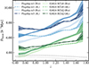 |
Fig. 1. Mean intergalactic separation in Flagship (blue colours) and GAEA (green colours) simulations for all considered models (m1 and m3 for Flagship, ECLH and ECLQ for GAEA). For each model, the fiducial galaxy selection based on the Hα flux (Hα) is compared to the stellar mass-based selection (M*). Shaded regions correspond to the standard deviation across five mocks for each model. Dotted and dashed grey lines represent the corresponding redshift uncertainties converted into distances for Flagship and GAEA simulations, respectively. GAEA models show smaller differences between each other and compared to the Flagship simulation models, in particular for the Hα selection of galaxies. Above z ∼ 0.9, the Hα selection follows the selection more closely, based on stellar mass for the Flagship simulation, with respect to GAEA. |
2.3.4.2. Stellar mass and Hα luminosity functions:
The stellar mass (SMF) and Hα luminosity functions (LF) for all Flagship and GAEA models are displayed in Fig. 2 in three different redshift bins. To highlight the impact of Hα flux selection on these observables, we also show the results for samples without any Hα flux limit. The SMFs of Flagship and GAEA models are compared with the COSMOS2020 observational dataset (Shuntov et al. 2022), while for the LFs the models are compared to data from the Emission Line COSMOS catalogue (Saito et al. 2020), HST-NICMOS (Shim et al. 2009), HST WISP (Colbert et al. 2013), and HiZELS (Sobral et al. 2013).
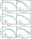 |
Fig. 2. Stellar mass (left) and Hα luminosity functions (right) in three redshift bins, 0.4 < z < 0.9 (top), 0.9 < z < 1.3 (middle), and 1.3 < z < 1.7 (bottom), in all models considered in this work for Hα flux limited samples (coloured solid lines) and for samples without any limit (coloured dashed lines). Black symbols correspond to observational data at these redshifts, COSMOS2020 (Shuntov et al. 2022) for stellar mass functions and the Emission Line COSMOS catalogue (Saito et al. 2020), HST-NICMOS (Shim et al. 2009), HST WISP (Colbert et al. 2013), and HiZELS (Sobral et al. 2013) for Hα luminosity functions. |
Overall, the SMFs of Flagship and GAEA galaxies without the Hα flux limit (dashed lines) agree well with the observational measurements in all redshift bins3. This is not surprising, particularly for GAEA, since the SMF was used to calibrate their models.
The application of an Hα flux limit translates non-trivially to the change in the SMF in a model-dependent way. The SMFs for the Hα flux-limited samples show a reduced amplitude at all stellar masses for all models except GAEA ECLH for which the SMFs overlap at the high-mass end (the stellar mass at which the deviation occurs depends on the redshift). Overall, the SMFs follow a qualitatively similar trend for all models. The steep increase at the high-mass end is followed by a shallower slope at intermediate masses and a downturn of the SMF at low masses. The stellar mass at which the SMFs start to decrease at the low-mass end increases with increasing redshift and depends on the model. For Flagship it corresponds to ∼109.5 M⊙, 109.5 M⊙, and 109.65 M⊙ in the three increasing redshift bins, while for GAEA the corresponding masses are slightly higher, particularly in the two highest redshift bins (109.75 M⊙ and 1010.15 M⊙).
The Hα LF of observed galaxies at low redshifts (0.4 < z < 0.9; Colbert et al. 2013; Saito et al. 2020) is well reproduced by Flagship, the model m3 in particular. This is expected, given that the LF of galaxies was among the observables used to calibrate the Flagship mocks. GAEA mocks reproduce reasonably well the LF of galaxies at the faint end, whereas they over-predict the number of observed galaxies at the bright end. At intermediate redshifts (0.9 < z < 1.3), the Hα LF of the observed galaxies (Shim et al. 2009; Colbert et al. 2013) lies well within the range spanned by the four galaxy mocks, making them a fairly good representation of galaxies at luminosities  , corresponding to the Hα flux limit of EDS at z = 1.3. At higher redshifts (1.3 < z < 1.7), the Hα LFs of all mocks under-predict observations (Colbert et al. 2013; Saito et al. 2020) below LHα ∼ 1042.8 erg s−1, while at higher luminosities, most models agree well with observations. GAEA in particular reproduces well the observed LF at the bright end in spite of the fact that this observable has not been used to calibrate the models.
We note that the drop (down turn) of the LF at the faint end for the Hα flux-limited sample is a consequence of the relatively large width of the redshift bins. The luminosity at which the two LFs (for full and Hα flux-limited samples) start to deviate corresponds to the Hα flux limit of the upper bound of each redshift bin. This corresponds to the Hα luminosity of 1040.51 erg s−1, 1041.37 erg s−1, 1041.77 erg s−1, and 1042.07 erg s−1, at redshifts 0.4, 0.9, 1.3, and 1.7, respectively.
2.3.4.3. Main sequence:
Figure 3 shows the relation between the stellar mass and star formation rate of galaxies in the Flagship and GAEA simulations in two redshift bins, 0.4 < z < 0.9 (top panels) and 0.9 < z < 1.8 (bottom panels). We only show models m3 and ECLH, but the results are similar for m1 and ECLQ. All galaxy mocks recover the expected correlation between the SFR and Hα luminosity. Comparison with the compilation of observational data from Popesso et al. (2023) confirms that, in general, there is good agreement between observations and simulations. The shape of the star-forming main sequence for Hα flux-limited sample (solid black lines) is better reproduced in GAEA compared to Flagship across a wide range of stellar masses in both redshift bins. However, both models show a shift compared to the observed main sequence. In GAEA, galaxies lie below, whereas in Flagship, they tend to be above the observed relation.
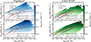 |
Fig. 3. Star-forming main sequence in the Flagship (left) and GAEA (right) simulations (models m3 and ECLH, respectively) at 0.4 < z < 0.9 (top) and 0.9 < z < 1.8 (bottom), color-coded by the Hα luminosity, which essentially correlates with SFR. The red lines correspond to the compilation of observational data presented in Popesso et al. (2023). The contours encompass 50% and 75% of the galaxy distribution for Hα flux-limited sample (solid lines) and for the sample without any limit (dashed lines). |
2.3.4.4. Galaxy clustering:
Figure 4 shows the two-point correlation functions of galaxies, relying on the Landy–Szalay estimator (Landy & Szalay 1993), in the redshift range 0.8 < z < 1.3 for the 5% Hα flux-brightest and the 5% least bright galaxies in the Flagship m3 and GAEA ECLH mocks. Similar results are found in Flagship m1 and GAEA ECLQ. In both simulations, the clustering is generally higher for the 5% brightest galaxies compared to their 5% lowest Hα flux counterparts at large separations (≳1 h−1 hMpc). At separations ≲1 h−1 hMpc, the 5% brightest galaxies in GAEA show reduced clustering with respect to their lower-brightness counterparts, whereas in Flagship, the clustering of the brightest galaxies continues to be higher, presumably better tracing the substructures. We note that galaxy clustering was among the constraints used during the construction of Flagship mocks to set the number of satellites and assign colour types to galaxies, while this information was not considered at all for the GAEA models. We note also that the considered redshift range bin is quite large. However, the median (and also mean) redshifts of the 5% highest and lowest Hα flux galaxies are comparable ( for Flagship m3 and GAEA ECLH;
  for the 5% highest and
  for the 5% lowest Hα flux sample in Flagship m1 and GAEA ECLQ). Therefore, the observed differences in the clustering of these populations are unlikely to be driven by their redshifts alone. We finally note that qualitatively similar results are found when considering 10% cut in the Hα flux, and/or for higher redshift range, e.g. 1.3 < z < 1.8.
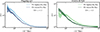 |
Fig. 4. Two-point correlation functions of galaxies in the redshift range 0.8 < z < 1.3 for galaxies with the 5% highest and lowest Hα flux in the Flagship m3 (left) and GAEA ECLH (right) mocks. Shaded regions correspond to jackknife error bars. At small separations (≲1 h−1 Mpc), brightest galaxies show enhanced clustering in Flagship compared to their low Hα flux counterparts, while the brightest galaxies in GAEA show comparable (or reduced) clustering to their lower brightness counterparts. At larger separations (≳1 h−1 Mpc), the brightest galaxies are more clustered compared to their low Hα flux counterparts in all mocks. |
2.4. Cosmic web reconstruction
To extract the cosmic web network, we rely on the publicly available and widely used structure finder DisPerSE (Sousbie 2011; Sousbie et al. 2011). To account for the redshift-space distortions that affect any 3D galaxy distribution relying on redshift-based distance measurements, we follow the method outlined in Kraljic et al. (2018). This approach has been previously adopted for the cosmic web reconstruction in 3D space using spectroscopic surveys, such as GAMA or SDSS (Kraljic et al. 2018, 2020b). Here, we only briefly describe its main steps.
To minimise the impact of redshift-space distortions induced by the random motions of galaxies within virialised haloes, the so-called Fingers of God (FoG) effect (e.g. Jackson 1972), we first need to identify the galaxy groups. This is done using an anisotropic friends of friends (FoF) algorithm that operates on the projected perpendicular and parallel separations of galaxies (see Treyer et al. 2018, for details on the group finder algorithm) calibrated on the Flagship and GAEA mock catalogues. Table 1 shows the resulting optimal linking lengths, in units of the mean intergalactic separation, for all models used in this work.
Optimal linking lengths (in units of the mean intergalactic separation).
The next step consists of the radial compression of the groups such that the dispersions of their member galaxies in transverse and radial directions are equal (see also e.g. Tegmark et al. 2004). The resulting isotropic galaxy distribution within the groups about their centres minimises the impact of elongated structures along the line-of-sight (i.e. the FoG effect) that could be misidentified as filaments of the cosmic web.
Finally, DisPerSE is used to coherently identify all the components of the cosmic web (i.e. voids, walls, filaments, and nodes) directly from the inhomogeneous distribution of galaxies, relying on discrete Morse theory (Forman 2001). To deal with such a discrete data set, DisPerSE builds on the Delaunay tessellation allowing one to provide a scale-free Delaunay Tessellation Field Estimator (DTFE; Schaap & van de Weygaert 2000) density and reconstruct the local topology. In this work we will consider the cosmic web reconstruction relying on both the non-weighted and stellar mass-weighted Delaunay tessellation. To deal with noisy data, such as galaxy catalogues, DisPerSE implements the concept of the topological persistence allowing to effectively filter out the topologically less robust features, i.e. features that would disappear or change after resampling of or adding a noise to the underlying field of the galaxy distribution. The level of filtering is controlled by the persistence threshold Nσ, such that higher values of Nσ select structures that are topologically more robust with respect to noise. The fiducial value used throughout this work is Nσ = 5. This higher value, compared to the more commonly used Nσ = 3, allows us to better highlight challenges of reconstructing cosmic web structures when working with Hα flux-limited, rather than stellar mass-limited, noisy data (see Sect. 3). Lastly, the cosmic web skeleton was smoothed in post-processing three times.
For illustration, Figs. 5 and 6 show a ∼40 h−1 hMpc thick slice of the distribution of galaxies within the redshift range 0.4 < z < 0.85 from the Flagship and GAEA mock catalogues (models m3 and ECLH, respectively) together with the corresponding network of filaments, reconstructed using unweighted Delaunay tessellation, for the reference catalogue, i.e. without FoG effect and with 100% completeness (top), after adding redshift error, 60% sampling and FoG effect (middle), and after correcting for the FoG effect (bottom). This visual inspection allows us to already identify some of the key factors impacting the quality of the cosmic web reconstruction, namely, the FoG effect, redshift uncertainty, and the incompleteness of the underlying galaxy sample. In the following, catalogues including redshift-space distortions are denoted with ’wFoG’ in the superscript (e.g. 𝒟wFoG), while catalogues with applied correction for the FoG effect include FoG, corr’ in the superscript (e.g. 𝒟FoG, corr).
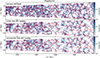 |
Fig. 5. Visualisation of a ∼40 h−1 Mpc thick slice of the galaxy distribution from the Flagship m3 mock and the corresponding cosmic web skeleton reconstructed without weighting Delaunay tessellation for the reference catalogue without the FoG effect, without added noise and with 100% completeness (𝒟; top), with the FoG, added redshift error and 60% sampling ( |


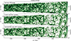 |
Fig. 6. Same as in Fig. 5, but for the GAEA ECLH mock. The higher galaxy number density of the GAEA ECLH mock compared to Flagship m3 (Fig. 5) can be clearly seen. |
3. Results
To assess the quality of the cosmic web reconstruction expected for the EDFs, we considered three different measures. These involve geometrical and topological properties of the cosmic web and transverse stellar-mass gradients of galaxies with respect to filaments of the cosmic web; namely, the observed and theoretically expected trend of increasing galaxies’ stellar mass with their decreasing distance from filaments.
3.1. The geometrical cosmic web measures
Geometrical measures of individual cosmic web components, such as the length of filaments, the area of walls, and the volume of voids, provide a straightforward way to assess the impact of different parameters on the quality of the cosmic web reconstruction. We explore in particular the impact of the FoG effect, redshift errors, and incompleteness of the galaxy sample.
Figure 7 shows the probability distribution function (PDF) of the lengths of filaments4, areas of walls, and volumes of voids for Flagship mock, m3 model (m1 model leads to the same conclusions) for the cosmic web reconstruction with (left) and without (right) the stellar mass-weighted Delaunay tessellation. Similarly, Fig. 8 presents the PDF of the filaments’ lengths for GAEA mock, model ECLH (the same conclusions apply to the ECLQ model). For walls and voids (not shown), qualitatively similar results and conclusions to those of Flagship are obtained.
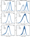 |
Fig. 7. PDF of filament lengths (top), wall areas (middle) and void volumes (bottom) for Flagship mocks (model m3) without redshift-space distortions for full (𝒟; solid grey lines), and 60% (𝒟60%; solid coloured lines) sampling, including the FoG effect ( |


As expected, the FoG effect has a strong impact on the filaments of the cosmic web, and much less so on its other components. When this effect is not corrected for, the reconstructed filaments tend to be too long as manifested by the shift of the distribution of filaments’ lengths towards larger values ( ) compared to the reference sample without redshift-space distortions (𝒟60%). After correcting for the FoG effect (
 ), the distributions of filaments’ lengths are in excellent agreement, both in terms of medians and overall shape for Flagship. For GAEA, the correction is not perfect, showing some residual deficit of long and excess of intermediate length filaments. We note, however, that the medians of the distributions are comparable.
Weighting the Delaunay tessellation by the stellar mass of galaxies turns out to be important for recovering a better agreement between the distributions before and after correcting for the FoG effect when the galaxy sample is not stellar mass-limited, as is the case for the EDS. As can be seen, the agreement between the distributions of filaments’ lengths does improve once the correction of the FoG effect is applied, but it is not as good as in the case of weighting. This is a direct consequence of the galaxy sample being Hα flux- rather than stellar mass-limited (see Fig. A.1). For stellar mass-limited galaxy samples the method used to deal with the FoG is efficient even without weighting the tessellation. The sample selection based on the Hα flux is also responsible for our failure to correct completely for the FoG effect seen for GAEA. The underlying reason is the inability to properly reconstruct galaxy groups, virialised structures responsible for small-scale redshift-space distortions, when the sample is not stellar mass-limited. As discussed in Sect. 2.3.4, Flagship and GAEA mocks show different clustering on small scales, with brightest galaxies tracing presumably more closely substructures in Flagship models, therefore resembling more the stellar mass selection.
The incompleteness of the galaxy sample manifests, as expected, by a shift of the distributions towards higher values (compare 𝒟60% vs. 𝒟 in Figs. 7 and 8), in particular for the filaments’ lengths. Walls and voids are impacted to a much lesser degree, especially when weighting is applied.
The redshift error, on top of the sample selection (whether it is stellar mass- or Hα flux-selected), strongly impacts our ability to correct for the FoG effect (see Fig. A.3). However, the correction works better for the stellar mass-limited sample.
In summary, the small-scale redshift-space distortions strongly impact the cosmic web reconstruction, filamentary network in particular, regardless of the sample selection and regardless of the weighting of the tessellation. The applied correction for the FoG effect works better for stellar mass-limited samples. On top of the sample selection, the redshift uncertainties hinder our ability to correct for the FoG effect.
3.2. Connectivity and multiplicity
The connectivity and multiplicity of the cosmic web, namely, the number of filaments that are globally and locally connected, respectively, to the nodes of the cosmic web, where massive galaxy groups and clusters predominantly reside, are interesting topological measures. They are expected to depend on the underlying cosmology and to impact the assembly of galaxies and hence their properties. It is therefore important to assess our ability to recover these quantities from the expected configuration for the EDFs.
We start by considering the distribution of connectivity, defined as the number of filaments connected to a given node of the cosmic web. Figure 9 shows the histograms of connectivity of central galaxies5 in the Hα flux-limited sample measured in the Flagship and GAEA mocks (models m3 and ECLH, respectively, but qualitatively similar results are obtained for models m1 and ECLQ). The FoG effect has a strong impact on the connectivity of galaxies at the nodes of the cosmic web (𝒟wFoG), modifying both the shape of the distribution, but also its median (indicated by a vertical line), regardless of the sample selection; namely, by including M*-limited samples (𝒟M*wFoG; see Fig. B.1). The correction of the FoG effect works very well for the M*-limited sample and reasonably well for the Hα flux-limited sample in terms of the overall shape of distributions, but also their mean and median values (see Tables B.1 and B.2). The weighting of the tessellation by stellar mass for the Hα flux-based selection (left panels of Fig. 9) tends to artificially increase connectivity even in the absence of redshift-space distortions, for example, with a median value of 8 (11) as opposed to a median value of 3 (5) without weighting for Flagship m3 (GAEA ECLH). For the M*-limited selection, the impact of weighting of the tessellation by stellar mass on the connectivity is very weak (see Fig. B.1). Adding redshift errors and incompleteness decreases the quality of the cosmic web reconstruction, in particular for the Hα-based selection (Fig. 10) due to the reduced ability to correct for FoG. In this configuration, stellar mass weighting of the tessellation improves the cosmic web reconstruction (see Tables B.1 and B.2).
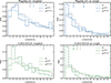 |
Fig. 9. PDFs of the connectivity of central galaxies for the Hα-limited selection of galaxies in the full sample without redshift error (𝒟) for Flagship model m3 (top) and GAEA model ECLH (bottom) mocks, with stellar mass weighting of the skeleton (left) and without weighting (right). In each panel, vertical lines indicate the medians of distributions. For a better visibility, the histograms are limited to the connectivity values below 14. Mean and median values for all distributions are reported in Tables B.1 and B.2. The redshift-space distortions have a strong impact on the connectivity of galaxies, but this effect that can be reasonably corrected for. |
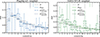 |
Fig. 10. PDFs of the connectivity of central galaxies for the Hα-limited selection of galaxies in the fiducial sample (𝒟noise, 60%; coloured lines) for Flagship model m3 (left) and GAEA model ECLH (right) mocks, with stellar mass weighting of the skeleton. The full sample without noise (𝒟) is shown for comparison (grey lines). In each panel, vertical lines indicate the medians of distributions and error bars correspond to the standard deviation across five mocks. For a better visibility, the histograms are limited to the connectivity values below 14. Mean and median values for all distributions are reported in Tables B.1 and B.2. Redshift errors and incompleteness of the sample decrease the quality of the cosmic web reconstruction, which can be improved by stellar mass weighting. |
Next, we explore the multiplicity and our ability to recover this local property of the cosmic web, defined as the connectivity minus the number of bifurcation points (i.e. points where filaments split, even though they are not extrema, Pogosyan et al. 2009), associated with each node. Figure 11 shows the multiplicity of central galaxies in Flagship and GAEA mocks (models m3 and ECLH, respectively, but almost identical results are obtained for the Flagship model m1 and the GAEA model ECLQ) for the fiducial sample (𝒟noise, 60%). Similarly to the connectivity, not correcting for the FoG effect modifies the distribution of multiplicity, but to a much lesser extent, in particular when the Delaunay tessellation is weighted by stellar mass. The mean and median values of the multiplicity agree very well across all mocks for weighted tessellation. For cosmic web reconstruction without weighting the tessellation, the correction of the FoG effect is needed to obtain good agreement between the distributions of multiplicity (Tables B.3–B.4). Qualitatively similar conclusions apply to the M*-limited samples. The multiplicity of the cosmic web therefore appears to be a more robust topological property compared to connectivity given its weak sensitivity to the FoG effect, redshift error, sample completeness, and its selection.
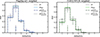 |
Fig. 11. PDFs of the multiplicity of central galaxies for an Hα-limited selection of galaxies in the fiducial sample (𝒟noise, 60%; coloured lines) for Flagship model m3 (left) and GAEA model ECLH (right) mocks, with stellar mass weighting of the skeleton. The full sample without noise (𝒟) is shown for a comparison (grey lines). In each panel, vertical lines indicate the medians of distributions and error bars correspond to the standard deviation across five mocks. The mean and median values for all distributions are reported in Tables B.3 and B.4. The multiplicity of the cosmic web shows only a weak sensitivity to the FoG effect, redshift error, and sample completeness. |
Beyond the statistical measurements of connectivity and multiplicity, it is of interest to explore these quantities as a function of different galaxy properties. In this work, we focus on stellar mass. Figure 12 shows the connectivity of central galaxies as a function of their stellar mass for the Flagship and GAEA mocks (models m3 and ECLH, respectively, with qualitatively similar conclusions for m1 and ECLQ) for the fiducial sample (𝒟noise, 60%). Regardless of the sample selection, i.e. Hα- or M*-limited (see Fig. B.2), central galaxies in the reference sample follow the expected trend, where the connectivity increases with increasing stellar mass, for the probed stellar mass range and when no weighting is applied prior to the cosmic web reconstruction (right panels of Fig. 12). Weighting of the Delaunay tessellation introduces a bias at lower stellar masses, in particular for the Hα-based galaxy selection, leading to an increase of the connectivity with decreasing stellar mass (left panels of Fig. 12). As already seen from the global distributions, the redshift-space distortions have a strong impact on the connectivity of the cosmic web. This leaves a clear signature in the form of a shift of the M*-connectivity relation towards higher values of connectivity, for mocks with FoG compared to the reference sample, regardless of the tessellation weighting. The applied correction of the FoG effect allows us to recover reasonably well the M*-connectivity relation of the reference samples, in particular for weighted tessellations. Weighting the tessellation by stellar mass is crucial for recovering the M*-connectivity trend if the sample is Hα flux-limited, in the presence of the redshift errors, and for reduced sampling, albeit with an introduced bias at lower masses.
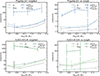 |
Fig. 12. Connectivity of central galaxies as a function of their stellar mass in Flagship model m3 (top) and GAEA model ECLH (bottom) mocks for the fiducial galaxy sample 𝒟noise, 60%, with stellar mass weighting of the skeleton (left) and without weighting (right). As expected, connectivity increases with stellar mass, with weighting of the Delaunay tessellation introducing a bias at lower stellar masses leading to reversed trend. Correction for the FoG effect is needed to recover reasonably well the M*-connectivity relation, in particular for weighted tessellations. |
Figure 13 shows the multiplicity of central galaxies as a function of their stellar mass for the Flagship and GAEA mocks (models m3 and ECLH, respectively, with qualitatively similar conclusions for m1 and ECLQ) for the fiducial sample (𝒟noise, 60%). As in the case of connectivity, the multiplicity of central galaxies increases with increasing stellar mass for galaxies in all reference catalogues (𝒟) regardless of sample selection (see Fig. B.3 for the M*-limited sample; 𝒟M*) and without tessellation weighting (see Fig. B.4). At the lowest stellar mass end (below 109.5 M⊙), accessible only in the Hα flux-selected samples, multiplicity tends to increase when stellar mass-weighted tessellation is used for the cosmic web reconstruction. Contrary to connectivity, the redshift-space distortions do not strongly modify the amplitude of the M*-and-multiplicity relation. The impact of FoG on this relation is overall very limited for the reconstruction with the stellar mass-weighted tessellation, but critically reduces our ability to recover the trend when the sample is Hα flux-limited (𝒟wFoG,  ) and no weighting is applied. The applied FoG correction significantly improves our ability to recover the M*-multiplicity relation in all mocks, but as for connectivity, the quality of this correction decreases with added redshift errors.
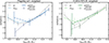 |
Fig. 13. Multiplicity of central galaxies as a function of their stellar mass in Flagship model m3 (left) and GAEA model ECLH (right) mocks for the fiducial sample, with stellar mass weighting of the skeleton. As for connectivity, multiplicity increases with M*, with a reversed trend at low M*. In contrast to connectivity, the redshift-space distortions do not strongly modify the amplitude of the M*-multiplicity relation. |
In summary, for Hα flux-limited samples, as in the case of EDF, the multiplicity appears to be a more robust quantity, compared to connectivity. Indeed, even without weighting the tessellation, and after applying a correction for the FoG effect, we are able to recover the M*-multiplicity relation in the presence of redshift error and reduced sampling. However, given that the range of multiplicity values is quite restrained, we anticipate that it might still be difficult to retrieve correlations between the multiplicity of galaxies located at nodes of the cosmic web and their properties beyond stellar mass (e.g. morphology or star formation activity).
3.3. Stellar-mass gradients
As explained by the theory of biased clustering (e.g. Kaiser 1984; Efstathiou et al. 1988), the mass of galaxies is expected to depend on their large-scale environment, such that more massive galaxies are preferentially formed in over-dense regions (e.g. Bond & Myers 1996; Pogosyan et al. 1996; Malavasi et al. 2017; Kraljic et al. 2018; Laigle et al. 2018). We go on to explore the stellar-mass gradients with respect to filaments of the cosmic web and our ability to recover this trend with the EDS below.
Figure 14 shows the PDFs of the distances of galaxies to their closest filament for the Flagship m3 model and for the reconstruction of the cosmic web with weighted tessellation as a function of stellar mass and redshift. The equivalent PDFs for the reconstruction without weighting are presented in Fig. C.2. Similar results are obtained for the Flagship m1 model and both GAEA models. The distances are normalised by the mean intergalactic separation to take into account the effect of decreasing the density of galaxies with increasing redshift. After accounting for these redshift variations, stellar-mass gradients, where more massive galaxies are preferentially located closer to filaments compared to their lower-mass counterparts, exhibit only minimal evolution in the redshift range 0.4 < z < 1.8, with galaxies typically found closer to the filaments of the cosmic web at lower redshifts.
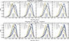 |
Fig. 14. PDFs of the closest filament’s distance, normalised by the redshift dependent mean intergalactic separation, for galaxies in the Flagship mock (model m3) in different stellar mass bins (coloured lines; with numbers indicating log10(M*/M⊙) values) and the cosmic web reconstructed using the stellar mass-weighted Delaunay tessellation. Stellar-mass gradients are shown as a function of redshift from the lowest redshift bin (left) to the highest one (right). Stellar-mass gradients, with more massive galaxies located closer to the filaments than their lower mass counterparts, present in the reference Hα flux-limited sample (𝒟; top), are recovered when the FoG correction is performed ( |

Stellar-mass gradients towards filaments of the cosmic web are recovered in the reference sample (𝒟, first rows of Figs. 14 and C.2) regardless of whether the weighting of Delaunay tessellation is applied or not. We note that the bimodality seen for the distributions without weights is due to our choice for a relatively high value of the persistence threshold Nσ applied to select filaments. This is caused by the removal of topologically less significant filaments for higher Nσ, which leaves some galaxies associated with filaments further away.
Reducing sample completeness weakens this signal (𝒟60%, Figs. C.1 and C.2), especially when the cosmic web is reconstructed without stellar mass-weighted tessellation. Redshift errors further reduce our ability to detect the stellar-mass gradients across the entire mass range ( , Fig. C.1), in particular for reconstructions without tessellation weighting. Correcting for the FoG effect does not significantly improve the strength of the signal (
 , second rows of Figs. 14 and C.2).
4. Discussion
4.1. Guidelines for cosmic web reconstruction with the spectroscopic Euclid Deep dataset
One of the major difficulties identified in this work hampering the reconstruction of the cosmic web in three dimensions is the galaxy selection function. An Hα flux-limited (rather than a stellar mass-limited selection of galaxies) is suboptimal for the reconstruction of the cosmic web in three dimensions. In addition, the redshift errors expected for the EDS further reduce the quality of the cosmic web reconstruction. In this section, we summarise and discuss possible choices to deal with these issues together with their implications.
Any cosmic web reconstruction in three dimensions employing galaxy redshift-based distances needs to account for the redshift-space distortions. Widely used methods to correct for such an effect on small scales depend on a reliable detection of galaxy groups and clusters. The optimisation of a group finder is typically performed on galaxy mocks designed to capture the specificities of a given survey. We have at our disposal two sets of mock catalogues, the Flagship and GAEA simulations, each providing two models of Hα flux of galaxies. As all these models reasonably represent galaxy populations at 0.4 < z < 1.8, based on comparisons with observational datasets of the galaxies’ main sequence, stellar mass, and Hα luminosity functions, we used them to optimise the anisotropic group finder.
However, due to inherent differences in the modelling of Hα flux, Flagship and GAEA show some fundamental differences; for example, in the clustering of galaxies on small scales (below ∼1 h−1 hMpc; see Fig. 4) or number density of galaxies across the entire redshift range (see Fig. 1). All of these non-trivial differences make it difficult to homogenise the cosmic web reconstruction. Consequently, we decided to treat each model as a plausible representation of our Universe and optimised the reconstruction process individually. The resulting optimal linking lengths are reported in Table 1. We note that these values are different for the Flagship and GAEA mocks, but they are reasonably close, not only to each other but also to the values adopted for the FoF algorithm-based group reconstruction method concentrating on lower redshift spectroscopic surveys (e.g. Robotham et al. 2011; Duarte & Mamon 2014; Treyer et al. 2018). This means that the exact choice of the linking lengths for the reconstruction of galaxy groups in the EDS will have to be made once the data are available on the basis of the comparison with the two mocks.
When reconstructing the cosmic web from discrete galaxy samples that are Hα flux- rather than stellar mass-limited, weighting the Delaunay tessellation by stellar mass of galaxies might improve the quality of the reconstruction, in particular in the presence of redshift errors with an RMS of 0.001(1 + z). However, this only holds for certain quantities. Among those explored in this work, geometrical cosmic web quantities (i.e. the length of filaments, the area of walls, and the volume of voids) are better recovered when stellar mass weighting is applied.
For topological cosmic web measurements, such as connectivity and multiplicity, the recommendation to apply weighing is less obvious. The main reason is that the stellar mass-weighted tessellation modifies the connectivity of the reconstructed filamentary network by typically shifting it towards higher values. Hence, the comparison with theoretical predictions and existing measurements from hydrodynamical simulations (e.g. Kraljic et al. 2020b; Galárraga-Espinosa et al. 2024) and low-redshift mass- or volume-limited samples (e.g. Kraljic et al. 2020b) becomes less obvious; this should be properly taken into account when interpreting any such connectivity measurement. However, stellar mass weighting helps to recover the M*-connectivity correlation. Interestingly, the multiplicity of the cosmic web seems to be very weakly affected by weighting, allowing us to reconstruct the correlation between the stellar mass of central galaxies and the number of locally connected filaments, as well as the global measure of the multiplicity such as its PDF. We therefore recommend using multiplicity rather than connectivity.
Finally, the segregation of galaxies by stellar mass with respect to their distance to the filaments of the cosmic web, as explored in this work, is found to be strongly impacted by the redshift error expected for the EDS. The stellar-mass gradients are recovered even without weighting by the stellar mass of galaxies. However, this signal is quite weak, and we anticipate that measuring gradients of quantities beyond stellar mass of galaxies, for example, gradients of the specific SFR (sSFR) would be very challenging in this regard. A significant improvement can be obtained by weighting the tessellation by stellar mass. Weighting the tessellation by stellar mass may seem to lead to stellar-mass gradients somewhat by construction. However, the stellar-mass gradients with respect to the filaments are naturally present and recovered in the reference sample without any weighting for the cosmic web reconstruction. In addition, the tests we conducted revealed that weighting by stellar masses randomly assigned to galaxies from the same catalogue significantly reduces the presence of stellar-mass gradients. We therefore conclude that while the stellar mass weighting of the tessellation clearly biases to some extent the cosmic web reconstruction (by construction more massive galaxies will follow the cosmic web more closely), the stellar-mass gradients are inherently present in the distribution of galaxies on large scales.
4.2. Science cases with Euclid Deep Survey
The current study focuses on the technical aspects of cosmic web reconstruction within EDS, with the aim of providing basic guidelines for future analysis. Validation has been performed by analysing some of the more fundamental properties of the cosmic web, with correlations involving filaments on the one hand and stellar mass of galaxies on the other. Euclid data provide the foundation to extend this analysis to other properties beyond their stellar mass, potentially allowing us to study the co-evolution of galaxies and the cosmic web at epochs close to cosmic noon.
It will be of particular interest to assess the impact of the cosmic web on the star formation of galaxies. Through measurements of the Hα flux of galaxies, Euclid will provide access to their SFR for the spectroscopic sample within the EDS. It will therefore be possible to perform the analysis of the gradients of the sSFR of galaxies with respect to the distance to filaments and walls of the cosmic web. At low redshifts, galaxies with lower sSFR (or redder colours) are found to be located closer to filaments and walls, compared to galaxies with higher sSFR (or bluer colours) at fixed M*. Qualitatively similar trends are found in cosmological hydrodynamical simulations, with such a behaviour persisting up to at least redshift z ∼ 1, and weakening or vanishing at z ∼ 2 (e.g. Xu et al. 2020; Hasan et al. 2023; Bulichi et al. 2024), with a hint of a reversal with increasing sSFR in the vicinity of filaments (Bulichi et al. 2024). Euclid will allow us to test these predictions, and extend to higher redshifts our knowledge on the impact of the cosmic web on the star formation activity of galaxies.
Low-redshift studies, both observational and numerical, also highlight the important role of connectivity (and multiplicity) of the cosmic web in shaping galaxy properties beyond their stellar mass. At fixed M*, galaxies at the nodes of the cosmic web with higher number of connected filaments tend to have lower sSFR and to be less rotationally supported compared to galaxies with lower connectivity (Kraljic et al. 2020b). As connectivity is a practical observational proxy for past and present accretion of galaxies and therefore controls their assembly history, it is of great importance to extend this kind of study to higher redshifts. Euclid will allow us to infer the cosmic evolution of connectivity (and multiplicity) of the cosmic web and its impact on various galaxy properties, such as sSFR and morphology, as well as metallicity, to name a few. In particular, detailed morphological information will be obtained from photometry (with various methods: profile-fitting, non-parametric estimates, deep learning; Euclid Collaboration: Bretonnière et al. 2023) provided by the VIS instrument (Euclid Collaboration: Cropper et al. 2025). The Euclid pipeline includes a model-fitting algorithm evaluated through the Euclid Morphology Challenge using simulated datasets. Euclid is expected to deliver robust structural parameters for more than 400 million galaxies, with a less than 10% scatter for single Sérsic profiles down to IE = 23 and double Sérsic profiles down to IE = 21. For complex morphologies, performance can be improved using the Zoobot convolutional neural network (CNN) and larger crowd-sourced datasets. Zoobot’s adaptability to new morphological labels was demonstrated with peculiar galaxies, highlighting its utility for detailed Euclid catalogues (Euclid Collaboration: Aussel et al. 2024).
Besides morphology measurements, the VIS instrument will provide precise estimates of the position angle of galaxies that jointly with access to large-scale structure will enable us to investigate the alignment of angular momentum (or spin) of galaxies with respect to the filaments and walls of the cosmic web. At low redshifts (z ≲ 0.2), statistical studies using data from the SDSS, SDSS-IV MaNGA and SAMI surveys revealed that rotationally supported, disk-dominated low-mass galaxies tend to have their spin aligned with their neighbouring filaments and walls, while bulge-dominated (S0-type) massive galaxies have their spin preferentially in the perpendicular direction (e.g. Tempel et al. 2013; Tempel & Libeskind 2013; Welker et al. 2020; Kraljic et al. 2021). As suggested by hydrodynamical cosmological simulations, such a spin alignment signal is expected to be stronger at z ≳ 1 (e.g. Dubois et al. 2014; Codis et al. 2018a; Wang et al. 2018; Kraljic et al. 2020a), making the EDS an ideal data set for measuring the 3D orientation of galaxies’ angular momentum with respect to large-scale filaments and walls at high redshift.
Understanding the co-evolution of galaxies and large-scale structure is of interest not only in the context of galaxy formation and evolution, but it is also of paramount importance for cosmology. An important example is the spin alignment of galaxies with regard to large-scale structure, as it is a known source of contamination for weak-lensing-based dark energy surveys (e.g. Chisari et al. 2017). Another example is cosmic connectivity and its evolution that is expected to depend on cosmology (e.g. Codis et al. 2018b; Mainieri et al. 2024; Boldrini & Laigle 2025) and, therefore, it could be an interesting probe of cosmological models beyond ΛCDM. Beyond connectivity, other cosmic web properties, such as exclusion zones present in the cross-correlations of critical points of the density field that were found to behave as standard rulers, represent a promising tool for constraining cosmological parameters (Shim et al. 2024).
4.3. Synergies with other surveys
Connecting the evolution of galaxies and the large-scale cosmic web requires spectroscopic surveys with high spatial sampling across a wide area in order to properly sample a wide range of cosmic environments. The EDS will in this regard be complementary to the PFS Galaxy Evolution survey (PFS hereafter; Greene et al. 2022). The PFS main continuum-selected sample of ∼3 × 10⁵ galaxies with J < 22.8 in the redshift range 0.7 ≲ z ≲ 1.7 will allow one to capture ∼90% of the population with M* ≳ 1010 M⊙. With 70% average completeness, PFS will enable the observation of multiple galaxies in groups with halo masses down to ∼1013 M⊙. This makes it ideal not only for studying the assembly history of galaxy groups, but also for the cosmic web-related analysis, thanks to an improved reconstruction of the large-scale structure (Kraljic et al., in prep.).
The EDS is also complementary to the main guaranteed time observation (GTO) MOONS extra-galactic survey at the VLT (MOONRISE; Maiolino et al. 2020), an upcoming massively multiplexed spectroscopic survey that enables the study of galaxy properties with rest-frame optical line coverage up to z ∼ 2. With its unique observing capabilities and strategy, MOONS is expected to capture the environment of galaxies across four orders of magnitude in over-density, from large under-dense void regions to high-density groups and clusters at z ∼ 1 − 2. This will, in turn, allow for the reconstruction of the cosmic web (particularly the filaments connected to galaxy clusters) and facilitate the study of their impact on galaxy properties at the peak of the cosmic SFR in the Universe.
In the comparable redshift range z ∼ 1 − 2, additional complementarity will be provided by the planned Nancy Grace Roman Space Telescope (Roman; Akeson et al. 2019). Galaxy samples from Roman’s deeper observations with the High-Latitude Wide-Area Survey (HLWAS; Wang et al. 2022), in particular its deep and ultra-deep tiers covering, respectively, ∼19 and ∼5 deg2 areas, are expected to allow for a reconstruction of the cosmic web with a mean galaxy number density comparable to that of EDS (Hasan et al. 2025). However, thanks to the larger wavelength coverage of Roman grisms, the emission lines [OIII] will be detectable beyond z ∼ 1.9, extending the Roman redshift coverage to z ∼ 2.8 (Zhai et al. 2021). This represents a true complementarity to Euclid, pushing potentially the cosmic web reconstruction in 3D to even higher redshifts.
Another potential complementarity with the EDS will be offered, at lower redshifts, by DESI, which is already collecting spectra (e.g. DESI Collaboration 2024, 2025). In particular, the DESI magnitude-limited Bright Galaxy Survey (BGS; Hahn et al. 2023), comprising approximately ten million galaxies over the redshift range 0 < z < 0.6, will provide a galaxy sample up to two magnitudes fainter than the SDSS Main Galaxy Sample (Strauss et al. 2002), with doubled median redshift (z ≈ 0.2). With significantly higher number density than any previous survey in this redshift range, spectra and photometry for ten million galaxies, BGS will enable measurements of their physical properties and the reconstruction of the cosmic web in three dimensions. This will in turn enable studies of the connection between the large-scale environment and galaxies, by focusing on their properties and statistics (e.g. the mass-metallicity relation, the star-forming main sequence, and stellar mass and luminosity functions at lower redshifts).
Finally, the Spectro-Photometer for the History of the Universe, Epoch of Reionization and Ices Explorer (SPHEREx, Bock et al. 2025) and the Vera C. Rubin Observatory’s Legacy Survey of Space and Time (LSST, Ivezić et al. 2019) will both provide photometric data on wavelength range complementary to the Euclid ground-based and NIR photometric filters. On the one hand, SPHEREx, launched on 11 March 2025, will provide an all-sky low-resolution spectro-photometric survey in 102 narrow-bands from 0.75 to 5.0 μm, at a depth comparable to the Euclid spectroscopic survey but with much lower spatial (6 2 pixels) and spectral (λ/Δλ = 35 − 130) resolutions. The EDFs and SPHEREx deep fields are planned to overlap (Doré et al. 2018), making SPHEREx a tool of choice to mitigate the fraction of catastrophic outliers in the Euclid spectroscopic survey, by providing additional constraints for line identification on a larger wavelength range. On the other hand, LSST, will provide a 18 000 deg2 coverage of the south hemisphere, thereby overlapping with EDFS and EDFF. In these fields, LSST will provide deep optical photometry in six filters ugrizy, covering the wavelength range 0.32–1.05 μm (in a range where Euclid has only one broad-band). This photometry could also be used to help tuning the spectroscopic solution of galaxies in the spectroscopic EDS. Beyond constraining the redshifts, these photometric data will be valuable in improving the stellar mass measurements of the Euclid galaxies, which, in turn, is pivotal to weighting the density field at the stage of skeleton extraction.
5. Conclusions
In this study, we investigated the quality of the reconstruction of the cosmic web with the expected spectroscopic dataset of galaxies in the EDFs in the redshift range 0.4 < z < 1.8, with an Hα flux limit of 6 × 10⁻¹⁷ erg cm−2 s−1. This analysis was carried out using the Flagship and GAEA mock galaxy catalogues. Our main findings are as follows:
-
Geometry of the cosmic web: The small-scale redshift-space distortions strongly impact the cosmic web reconstruction, and its filamentary network in particular, regardless of the sample selection (Hα flux- or M*-limited) and regardless of what weighting of the tessellation by the stellar mass of galaxies is chosen. The correction applied for the FoG effect works better for stellar mass-limited samples. In addition to sample selection, the redshift uncertainties hinder our ability to correct for the FoG effect.
-
Connectivity of the cosmic web: For the overall properties of the PDF of the connectivity, the correction of the FoG effect works very well for the M*-limited sample and reasonably well for the Hα flux-limited sample. Weighting the tessellation by stellar mass for the Hα flux-based selection artificially enhances the connectivity, even in the absence of redshift-space distortions. Adding noise and incompleteness reduces the quality of the cosmic web reconstruction for both Hα-based and M*-based galaxy selections, due to the diminished ability to correct for FoG effects. In this configuration, stellar mass weighting of the tessellation significantly improves the cosmic web reconstruction, particularly for an Hα-based galaxy selection. Weighting is similarly crucial to recover the M*-connectivity relation when the sample is Hα flux-limited, in the presence of redshift errors, and for reduced sampling.
-
Multiplicity of the cosmic web: For Hα flux-limited samples (in contrast to the case of M*-limited samples), the multiplicity appears to be a more robust quantity compared to the connectivity. Even without weighting the tessellation, the applied correction for the FoG effect enables us to recover the M*-multiplicity relation. This holds true even in the presence of redshift errors and reduced sampling.
-
Stellar-mass gradients: In cases where more massive galaxies are preferentially located closer to filaments compared to their lower-mass counterparts, stellar-mass gradients can be recovered regardless of whether the tessellation is weighted by stellar mass. However, the redshift error and limited sampling significantly weaken the strength of the measured signal for the Hα flux-limited sample in the absence of tessellation weighting.
In this work, we performed the cosmic web reconstruction in three dimensions using simulated spectroscopic redshifts in the range 0.4 < z < 1.8, expected in EDFs. The reconstruction methodology will therefore be applicable once the EDS data will be available and the performance of spectroscopic measurements fully assessed in this redshift range. The first results using the Euclid Quick Data Release (Q1) of the Spectroscopic Processing Functions of the Euclid pipeline (Euclid Collaboration: Le Brun et al. 2026) in the redshift range 0.9 < z < 1.8 are promising. It was shown that a success rate above 80%, and excellent redshift precision (∼10−3) and accuracy (better than 3 × 10⁻⁵) can be reached in only one visit. The final EDS will be made of about 40 visits and with much better performance.
The analysis of the cosmic web in two dimensions using photometric redshifts from the Q1 release, focussed on the galaxy morphology and shape alignments at 0.5 < z < 0.9, is presented in Euclid Collaboration: Laigle et al. (2026), while in Euclid Collaboration: Gouin et al. (2026), the focus is on cosmic connectivity of galaxy clusters at 0.2 < z < 0.7.
The present work is centred on the technical aspects of cosmic web reconstruction, with the goal of providing guidelines for future applications to real data. For this reason, we specifically only considered trends with the stellar mass of galaxies, leaving the exploration of the impact of the cosmic web on other galaxy properties for future studies. Euclid will enable such investigations for the first time across cosmic time, up to z ≈ 1.8.
Acknowledgments
The Euclid Consortium acknowledges the European Space Agency and a number of agencies and institutes that have supported the development of Euclid, in particular the Agenzia Spaziale Italiana, the Austrian Forschungsförderungsgesellschaft funded through BMIMI, the Belgian Science Policy, the Canadian Euclid Consortium, the Deutsches Zentrum für Luft- und Raumfahrt, the DTU Space and the Niels Bohr Institute in Denmark, the French Centre National d’Etudes Spatiales, the Fundação para a Ciência e a Tecnologia, the Hungarian Academy of Sciences, the Ministerio de Ciencia, Innovación y Universidades, the National Aeronautics and Space Administration, the National Astronomical Observatory of Japan, the Netherlandse Onderzoekschool Voor Astronomie, the Norwegian Space Agency, the Research Council of Finland, the Romanian Space Agency, the State Secretariat for Education, Research, and Innovation (SERI) at the Swiss Space Office (SSO), and the United Kingdom Space Agency. A complete and detailed list is available on the Euclid web site (www.euclid-ec.org). This work has made use of CosmoHub, developed by PIC (maintained by IFAE and CIEMAT) in collaboration with ICE-CSIC. CosmoHub received funding from the Spanish government (MCIN/AEI/10.13039/501100011033), the EU NextGeneration/PRTR (PRTR-C17.I1), and the Generalitat de Catalunya. This work is partially supported by the grant SEGAL ANR-19-CE31-0017 of the French Agence Nationale de la Recherche. This research has made use of computing facilities operated by CeSAM data centre at LAM, Marseille, France. We thank Stéphane Rouberol for the smooth running of the Infinity cluster, where part of the computations was performed.
References
- Abazajian, K. N., Adelman-McCarthy, J. K., Agüeros, M. A., et al. 2009, ApJS, 182, 543 [Google Scholar]
- Akeson, R., Armus, L., Bachelet, E., et al. 2019, arXiv e-prints [arXiv:1902.05569] [Google Scholar]
- Angulo, R. E., Zennaro, M., Contreras, S., et al. 2021, MNRAS, 507, 5869 [NASA ADS] [CrossRef] [Google Scholar]
- Baldry, I. K., Balogh, M. L., Bower, R. G., et al. 2006, MNRAS, 373, 469 [Google Scholar]
- Bamford, S. P., Nichol, R. C., Baldry, I. K., et al. 2009, MNRAS, 393, 1324 [NASA ADS] [CrossRef] [Google Scholar]
- Barsanti, S., Colless, M., Welker, C., et al. 2022, MNRAS, 516, 3569 [NASA ADS] [CrossRef] [Google Scholar]
- Behroozi, P. S., Wechsler, R. H., & Wu, H.-Y. 2013, ApJ, 762, 109 [NASA ADS] [CrossRef] [Google Scholar]
- Blanton, M. R., Hogg, D. W., Bahcall, N. A., et al. 2003a, ApJ, 594, 186 [NASA ADS] [CrossRef] [Google Scholar]
- Blanton, M. R., Hogg, D. W., Bahcall, N. A., et al. 2003b, ApJ, 592, 819 [Google Scholar]
- Blanton, M. R., Lupton, R. H., Schlegel, D. J., et al. 2005, ApJ, 631, 208 [Google Scholar]
- Bock, J. J., Aboobaker, A. M., Adamo, J., et al. 2025, ApJ, accepted [arXiv:2511.02985] [Google Scholar]
- Boldrini, P., & Laigle, C. 2025, A&A, 700, A182 [NASA ADS] [CrossRef] [EDP Sciences] [Google Scholar]
- Bond, J. R., & Myers, S. T. 1996, ApJS, 103, 1 [NASA ADS] [CrossRef] [Google Scholar]
- Bond, J. R., Kofman, L., & Pogosyan, D. 1996, Nature, 380, 603 [NASA ADS] [CrossRef] [Google Scholar]
- Bulichi, T.-E., Davé, R., & Kraljic, K. 2024, MNRAS, 529, 2595 [NASA ADS] [CrossRef] [Google Scholar]
- Burton, C. S., Jarvis, M. J., Smith, D. J. B., et al. 2013, MNRAS, 433, 771 [Google Scholar]
- Calzetti, D., Armus, L., Bohlin, R. C., et al. 2000, ApJ, 533, 682 [NASA ADS] [CrossRef] [Google Scholar]
- Carretero, J., Tallada, P., Casals, J., et al. 2017, in Proceedings of the European Physical Society Conference on High Energy Physics. 5–12 July, 488 [Google Scholar]
- Chabrier, G. 2003, PASP, 115, 763 [Google Scholar]
- Chen, Y.-C., Ho, S., Mandelbaum, R., et al. 2017, MNRAS, 466, 1880 [NASA ADS] [CrossRef] [Google Scholar]
- Chisari, N. E., Koukoufilippas, N., Jindal, A., et al. 2017, MNRAS, 472, 1163 [Google Scholar]
- Codis, S., Pichon, C., & Pogosyan, D. 2015, MNRAS, 452, 3369 [Google Scholar]
- Codis, S., Jindal, A., Chisari, N. E., et al. 2018a, MNRAS, 481, 4753 [Google Scholar]
- Codis, S., Pogosyan, D., & Pichon, C. 2018b, MNRAS, 479, 973 [Google Scholar]
- Colbert, J. W., Teplitz, H., Atek, H., et al. 2013, ApJ, 779, 34 [NASA ADS] [CrossRef] [Google Scholar]
- Colless, M., Dalton, G., Maddox, S., et al. 2001, MNRAS, 328, 1039 [Google Scholar]
- Cranmer, K., Brehmer, J., & Louppe, G. 2020, Proc. Natl. Acad. Sci., 117, 30055 [Google Scholar]
- Crone Odekon, M., Hallenbeck, G., Haynes, M. P., et al. 2018, ApJ, 852, 142 [NASA ADS] [CrossRef] [Google Scholar]
- Cucciati, O., Iovino, A., Kovač, K., et al. 2010, A&A, 524, A2 [NASA ADS] [CrossRef] [EDP Sciences] [Google Scholar]
- Cucciati, O., Davidzon, I., Bolzonella, M., et al. 2017, A&A, 602, A15 [NASA ADS] [CrossRef] [EDP Sciences] [Google Scholar]
- Darragh Ford, E., Laigle, C., Gozaliasl, G., et al. 2019, MNRAS, 489, 5695 [Google Scholar]
- Davis, M., & Geller, M. J. 1976, ApJ, 208, 13 [NASA ADS] [CrossRef] [Google Scholar]
- Davis, M., Huchra, J., Latham, D. W., & Tonry, J. 1982, ApJ, 253, 423 [NASA ADS] [CrossRef] [Google Scholar]
- de Lapparent, V., Geller, M. J., & Huchra, J. P. 1986, ApJ, 302, L1 [Google Scholar]
- De Lucia, G., Tornatore, L., Frenk, C. S., et al. 2014, MNRAS, 445, 970 [Google Scholar]
- DESI Collaboration (Aghamousa, A., et al.) 2016, arXiv e-prints [arXiv:1611.00036] [Google Scholar]
- DESI Collaboration (Adame, A. G., et al.) 2024, AJ, 168, 58 [NASA ADS] [CrossRef] [Google Scholar]
- DESI Collaboration (Abdul-Karim, M., et al.) 2025, ApJ, submitted [arXiv:2503.14745] [Google Scholar]
- Donnan, C. T., Tojeiro, R., & Kraljic, K. 2022, Nat. Astron., 6, 599 [NASA ADS] [CrossRef] [Google Scholar]
- Doré, O., Werner, M. W., Ashby, M. L. N., et al. 2018, arXiv e-prints [arXiv:1805.05489] [Google Scholar]
- Dressler, A. 1980, ApJ, 236, 351 [Google Scholar]
- Dressler, A., Oemler, A., Jr., Couch, W. J., et al. 1997, ApJ, 490, 577 [NASA ADS] [CrossRef] [Google Scholar]
- Driver, S. P., Hill, D. T., Kelvin, L. S., et al. 2011, MNRAS, 413, 971 [Google Scholar]
- Duarte, M., & Mamon, G. A. 2014, MNRAS, 440, 1763 [CrossRef] [Google Scholar]
- Dubois, Y., Pichon, C., Welker, C., et al. 2014, MNRAS, 444, 1453 [Google Scholar]
- Efstathiou, G., Frenk, C. S., White, S. D. M., & Davis, M. 1988, MNRAS, 235, 715 [NASA ADS] [CrossRef] [Google Scholar]
- Einasto, M., Deshev, B., Tenjes, P., et al. 2020, A&A, 641, A172 [NASA ADS] [CrossRef] [EDP Sciences] [Google Scholar]
- Einasto, M., Kipper, R., Tenjes, P., et al. 2021, A&A, 649, A51 [NASA ADS] [CrossRef] [EDP Sciences] [Google Scholar]
- Euclid Collaboration (Aussel, B., et al.) 2024, A&A, 689, A274 [NASA ADS] [CrossRef] [EDP Sciences] [Google Scholar]
- Euclid Collaboration (Bretonnière, H., et al.) 2023, A&A, 671, A102 [NASA ADS] [CrossRef] [EDP Sciences] [Google Scholar]
- Euclid Collaboration (Castander, F., et al.) 2025, A&A, 697, A5 [Google Scholar]
- Euclid Collaboration (Cropper, M., et al.) 2025, A&A, 697, A2 [Google Scholar]
- Euclid Collaboration (Malavasi, N., et al.) 2025, A&A, submitted [arXiv:2508.15915] [Google Scholar]
- Euclid Collaboration (McPartland, C. J. R., et al.) 2025, A&A, 695, A259 [Google Scholar]
- Euclid Collaboration (Mellier, Y., et al.) 2025, A&A, 697, A1 [Google Scholar]
- Euclid Collaboration (Scaramella, R., et al.) 2022, A&A, 662, A112 [NASA ADS] [CrossRef] [EDP Sciences] [Google Scholar]
- Euclid Collaboration (Zalesky, L., et al.) 2025, A&A, 695, A229 [Google Scholar]
- Euclid Collaboration (Copin, Y., et al.) 2026 A&A, in press, https://doi.org/10.1051/0004-6361/202554627 [Google Scholar]
- Euclid Collaboration (Gouin, C., et al.) 2026, A&A, in press, https://doi.org/10.1051/0004-6361/202554655 [Google Scholar]
- Euclid Collaboration (Laigle, C., et al.) 2026 A&A, in press, https://doi.org/10.1051/0004-6361/202554651 [Google Scholar]
- Euclid Collaboration (Le Brun, V., et al.) 2026 A&A, https://doi.org/10.1051/0004-6361/202554607 [Google Scholar]
- Fontanot, F., Hirschmann, M., & De Lucia, G. 2017, ApJ, 842, L14 [Google Scholar]
- Fontanot, F., De Lucia, G., Hirschmann, M., et al. 2020, MNRAS, 496, 3943 [CrossRef] [Google Scholar]
- Forman, R. 2001, Sém. Lothar. Combin., 48 [Google Scholar]
- Galárraga-Espinosa, D., Cadiou, C., Gouin, C., et al. 2024, A&A, 684, A63 [NASA ADS] [CrossRef] [EDP Sciences] [Google Scholar]
- Goto, T., Yamauchi, C., Fujita, Y., et al. 2003, MNRAS, 346, 601 [NASA ADS] [CrossRef] [Google Scholar]
- Greene, J., Bezanson, R., Ouchi, M., Silverman, J., & the PFS Galaxy Evolution Working Group 2022, arXiv e-prints [arXiv:2206.14908] [Google Scholar]
- Guzzo, L., Scodeggio, M., Garilli, B., et al. 2014, A&A, 566, A108 [NASA ADS] [CrossRef] [EDP Sciences] [Google Scholar]
- Hahn, C., Wilson, M. J., Ruiz-Macias, O., et al. 2023, AJ, 165, 253 [CrossRef] [Google Scholar]
- Hamaus, N., Aubert, M., Pisani, A., et al. 2022, A&A, 658, A20 [NASA ADS] [CrossRef] [EDP Sciences] [Google Scholar]
- Hasan, F., Burchett, J. N., Abeyta, A., et al. 2023, ApJ, 950, 114 [NASA ADS] [CrossRef] [Google Scholar]
- Hasan, F., Zhang, H., Pandya, V., et al. 2025, ApJ, submitted [arXiv:2509.23549] [Google Scholar]
- Hirschmann, M., De Lucia, G., & Fontanot, F. 2016, MNRAS, 461, 1760 [Google Scholar]
- Hou, J., Dizgah, A. M., Hahn, C., et al. 2024, Phys. Rev. D, 109, 103528 [NASA ADS] [CrossRef] [Google Scholar]
- Ivezić, Ž., Kahn, S. M., Tyson, J. A., et al. 2019, ApJ, 873, 111 [Google Scholar]
- Jackson, J. C. 1972, MNRAS, 156, 1P [CrossRef] [Google Scholar]
- Jones, D. H., Saunders, W., Colless, M., et al. 2004, MNRAS, 355, 747 [NASA ADS] [CrossRef] [Google Scholar]
- Jones, D. H., Read, M. A., Saunders, W., et al. 2009, MNRAS, 399, 683 [Google Scholar]
- Kaiser, N. 1984, ApJ, 284, L9 [NASA ADS] [CrossRef] [Google Scholar]
- Kennicutt, R. C., Jr. 1998, ARA&A, 36, 189 [Google Scholar]
- Kennicutt, R. C., Jr., Tamblyn, P., & Congdon, C. E. 1994, ApJ, 435, 22 [Google Scholar]
- Kirshner, R. P., Oemler, A., Jr., Schechter, P. L., & Shectman, S. A. 1981, ApJ, 248, L57 [NASA ADS] [CrossRef] [Google Scholar]
- Kleiner, D., Pimbblet, K. A., Jones, D. H., Koribalski, B. S., & Serra, P. 2017, MNRAS, 466, 4692 [Google Scholar]
- Klypin, A. A., & Shandarin, S. F. 1983, MNRAS, 204, 891 [NASA ADS] [Google Scholar]
- Klypin, A., & Shandarin, S. F. 1993, ApJ, 413, 48 [NASA ADS] [CrossRef] [Google Scholar]
- Kobayashi, Y., Nishimichi, T., Takada, M., & Miyatake, H. 2022, Phys. Rev. D, 105, 083517 [CrossRef] [Google Scholar]
- Kraljic, K., Arnouts, S., Pichon, C., et al. 2018, MNRAS, 474, 547 [Google Scholar]
- Kraljic, K., Davé, R., & Pichon, C. 2020a, MNRAS, 493, 362 [NASA ADS] [CrossRef] [Google Scholar]
- Kraljic, K., Pichon, C., Codis, S., et al. 2020b, MNRAS, 491, 4294 [Google Scholar]
- Kraljic, K., Duckworth, C., Tojeiro, R., et al. 2021, MNRAS, 504, 4626 [NASA ADS] [CrossRef] [Google Scholar]
- Krolewski, A., Ho, S., Chen, Y.-C., et al. 2019, ApJ, 876, 52 [NASA ADS] [CrossRef] [Google Scholar]
- Kuutma, T., Tamm, A., & Tempel, E. 2017, A&A, 600, L6 [NASA ADS] [CrossRef] [EDP Sciences] [Google Scholar]
- Laigle, C., Pichon, C., Arnouts, S., et al. 2018, MNRAS, 474, 5437 [Google Scholar]
- Landy, S. D., & Szalay, A. S. 1993, ApJ, 412, 64 [Google Scholar]
- Laureijs, R., Amiaux, J., Arduini, S., et al. 2011, ESA/SRE(2011)12, [arXiv:1110.3193] [Google Scholar]
- Lee, J., & Erdogdu, P. 2007, ApJ, 671, 1248 [Google Scholar]
- Lee, K.-G., & White, M. 2016, ApJ, 831, 181 [NASA ADS] [CrossRef] [Google Scholar]
- Libeskind, N. I., van de Weygaert, R., Cautun, M., et al. 2018, MNRAS, 473, 1195 [NASA ADS] [CrossRef] [Google Scholar]
- Lynden-Bell, D. 1964, ApJ, 139, 1195 [Google Scholar]
- Madau, P., & Dickinson, M. 2014, ARA&A, 52, 415 [Google Scholar]
- Mainieri, V., Anderson, R. I., Brinchmann, J., et al. 2024, arXiv e-prints [arXiv:2403.05398] [Google Scholar]
- Maiolino, R., Cirasuolo, M., Afonso, J., et al. 2020, Messenger, 180, 24 [Google Scholar]
- Malavasi, N., Arnouts, S., Vibert, D., et al. 2017, MNRAS, 465, 3817 [Google Scholar]
- McCullough, J., Gruen, D., Amon, A., et al. 2024, MNRAS, 531, 2582 [NASA ADS] [CrossRef] [Google Scholar]
- Musso, M., Cadiou, C., Pichon, C., et al. 2018, MNRAS, 476, 4877 [Google Scholar]
- Pahwa, I., Libeskind, N. I., Tempel, E., et al. 2016, MNRAS, 457, 695 [NASA ADS] [CrossRef] [Google Scholar]
- Pogosyan, D., Bond, J. R., Kofman, L., & Wadsley, J. 1996, AAS Meet. Abstr., 189, 13.03 [Google Scholar]
- Pogosyan, D., Pichon, C., Gay, C., et al. 2009, MNRAS, 396, 635 [NASA ADS] [CrossRef] [Google Scholar]
- Popesso, P., Concas, A., Cresci, G., et al. 2023, MNRAS, 519, 1526 [Google Scholar]
- Potter, D., & Stadel, J. 2016, Astrophysics Source Code Library [record ascl:1609.016] [Google Scholar]
- Pozzetti, L., Hirata, C. M., Geach, J. E., et al. 2016, A&A, 590, A3 [NASA ADS] [CrossRef] [EDP Sciences] [Google Scholar]
- Ravoux, C., Armengaud, E., Walther, M., et al. 2020, JCAP, 07, 010 [Google Scholar]
- Robotham, A. S. G., Norberg, P., Driver, S. P., et al. 2011, MNRAS, 416, 2640 [NASA ADS] [CrossRef] [Google Scholar]
- Saito, S., de la Torre, S., Ilbert, O., et al. 2020, MNRAS, 494, 199 [NASA ADS] [CrossRef] [Google Scholar]
- Sarron, F., Adami, C., Durret, F., & Laigle, C. 2019, A&A, 632, A49 [NASA ADS] [CrossRef] [EDP Sciences] [Google Scholar]
- Schaap, W. E., & van de Weygaert, R. 2000, A&A, 363, L29 [Google Scholar]
- Schäfer, B. M. 2009, Int. J. Mod. Phys. D, 18, 173 [Google Scholar]
- Shectman, S. A., Landy, S. D., Oemler, A., et al. 1996, ApJ, 470, 172 [NASA ADS] [CrossRef] [Google Scholar]
- Shim, H., Colbert, J., Teplitz, H., et al. 2009, ApJ, 696, 785 [NASA ADS] [CrossRef] [Google Scholar]
- Shim, J., Pichon, C., Pogosyan, D., et al. 2024, MNRAS, 528, 1604 [Google Scholar]
- Shuntov, M., McCracken, H. J., Gavazzi, R., et al. 2022, A&A, 664, A61 [NASA ADS] [CrossRef] [EDP Sciences] [Google Scholar]
- Smith, R., Hwang, H. S., Kraljic, K., et al. 2023, MNRAS, 525, 4685 [NASA ADS] [CrossRef] [Google Scholar]
- Sobral, D., Smail, I., Best, P. N., et al. 2013, MNRAS, 428, 1128 [NASA ADS] [CrossRef] [Google Scholar]
- Sousbie, T. 2011, MNRAS, 414, 350 [NASA ADS] [CrossRef] [Google Scholar]
- Sousbie, T., Pichon, C., & Kawahara, H. 2011, MNRAS, 414, 384 [NASA ADS] [CrossRef] [Google Scholar]
- Springel, V., Yoshida, N., & White, S. D. M. 2001, New Astron., 6, 79 [Google Scholar]
- Springel, V., White, S. D. M., Jenkins, A., et al. 2005, Nature, 435, 629 [Google Scholar]
- Strauss, M. A., Weinberg, D. H., Lupton, R. H., et al. 2002, AJ, 124, 1810 [Google Scholar]
- Tallada, P., Carretero, J., Casals, J., et al. 2020, Astron. Comput., 32, 100391 [Google Scholar]
- Tegmark, M., Blanton, M. R., Strauss, M. A., et al. 2004, ApJ, 606, 702 [Google Scholar]
- Tempel, E., & Libeskind, N. I. 2013, ApJ, 775, L42 [NASA ADS] [CrossRef] [Google Scholar]
- Tempel, E., Stoica, R. S., & Saar, E. 2013, MNRAS, 428, 1827 [NASA ADS] [CrossRef] [Google Scholar]
- Treyer, M., Kraljic, K., Arnouts, S., et al. 2018, MNRAS, 477, 2684 [NASA ADS] [CrossRef] [Google Scholar]
- Wang, P., Guo, Q., Kang, X., & Libeskind, N. I. 2018, ApJ, 866, 138 [NASA ADS] [CrossRef] [Google Scholar]
- Wang, Y., Zhai, Z., Alavi, A., et al. 2022, ApJ, 928, 1 [Google Scholar]
- Welker, C., Bland-Hawthorn, J., van de Sande, J., et al. 2020, MNRAS, 491, 2864 [NASA ADS] [CrossRef] [Google Scholar]
- Winkel, N., Pasquali, A., Kraljic, K., et al. 2021, MNRAS, 505, 4920 [CrossRef] [Google Scholar]
- Xu, W., Guo, Q., Zheng, H., et al. 2020, MNRAS, 498, 1839 [Google Scholar]
- York, D. G., Adelman, J., Anderson, J. E., Jr., et al. 2000, AJ, 120, 1579 [NASA ADS] [CrossRef] [Google Scholar]
- Zehavi, I., Zheng, Z., Weinberg, D. H., et al. 2011, ApJ, 736, 59 [NASA ADS] [CrossRef] [Google Scholar]
- Zel’dovich, Y. B. 1970, A&A, 5, 84 [NASA ADS] [Google Scholar]
- Zhai, Z., Wang, Y., Benson, A., et al. 2021, arXiv e-prints [arXiv:2109.12216] [Google Scholar]
- Zhang, Y., Yang, X., Wang, H., et al. 2013, ApJ, 779, 160 [NASA ADS] [CrossRef] [Google Scholar]
- Zhang, Y., Yang, X., Wang, H., et al. 2015, ApJ, 798, 17 [Google Scholar]
- Zoldan, A., De Lucia, G., Xie, L., Fontanot, F., & Hirschmann, M. 2017, MNRAS, 465, 2236 [NASA ADS] [CrossRef] [Google Scholar]
Completeness is defined as the fraction of objects recovered with a correct redshift from a full sample above a certain intrinsic flux limit and in a certain redshift range, while purity is the fraction of correctly measured redshifts in the recovered sample.
We note that we have not transformed the stellar masses of mock galaxies to units of the Hubble constant used in the observed galaxy catalogues.
In practice, half length of filaments, measured as the curvilinear distance between filament-type saddle points and maxima, the nodes of the cosmic web.
We focus on central galaxies to limit the complications due to the non-linear nature of the satellite population and to ease the comparison with theoretical predictions (for a more detailed discussion on the effect of satellites on connectivity, see Kraljic et al. 2020b).
Appendix A: Cosmic web statistics
Figure A.1 illustrates the effect of the selection function of galaxies and the mass weighting of the Delaunay tessellation on the distribution of filament lengths in the Flagship m3 model (see Fig. A.2 for the GAEA ECLH model with weighting). For the Hα-limited samples (left panels), weighting of the tessellation by stellar mass is necessary to correct for the FoG effect (compare the top left and bottom left panels). For a M*-limited sample (right panels), weighting is not needed to obtain a good agreement for the distribution of filaments’ length after correcting for the FoG effect (compare top right and middle right panels). This behaviour is recovered in all models used in this work. Figure A.3 highlights the effect of the reduced sampling on the distribution of filament lengths. As expected, reduced sampling (60 %, as estimated for the EDF) shifts the distribution of lengths of filaments to higher values, regardless of sample selection (Hα- and M*-limited sample, left and right panels, respectively).
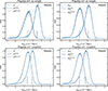 |
Fig. A.1. PDF of filament lengths for Hα- (left) and stellar mass-limited (right) samples. Top and bottom panels compare non-weighted and weighted tessellations, respectively, for the Flagship m3 model. Vertical lines indicate the medians of distributions. Shaded regions correspond to the bootstrap error bars. For the stellar mass-limited galaxy sample, weighting of the Delaunay tessellation for the cosmic web reconstruction is not required to obtain a good agreement for the distribution of filaments’ length. |
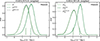 |
Fig. A.2. Same as in Fig. A.1 (bottom) i.e. using the stellar mass-weighted tessellation for the cosmic web reconstruction, but for the GAEA ECLH model. |
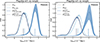 |
Fig. A.3. PDF of filaments’ length for stellar mass-limited (left) and Hα-limited (right) samples with 60 % sampling. |
Appendix B: Connectivity and multiplicity
Figure B.1 shows the PDFs of the connectivity of central galaxies for M*- limited selection of galaxies in the full sample without redshift error (𝒟) for Flagship (model m3, top panels) and GAEA (model ECLH, bottom panels), with stellar mass weighting of the Delaunay tessellation (left) and without weighting (right). The stellar mass weighting impacts the PDF of the connectivity to a much lesser degree when the galaxy sample is M*-limited compared to an Hα-limited selection. After correcting for the FoG effect, the shape of the distributions and their medians (vertical lines) are in very good agreement with the measurements in the absence of redshift-space distortions without tessellation weighting for both Flagship and GAEA. Stellar mass weighting introduces some spurious effects, preventing us from completely correcting for the FoG effect in GAEA. However, the distribution of the connectivity and its median are substantially improved. The mean and median values of connectivity for all mocks and selections are reported in Tables B.1 and B.2.
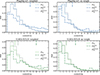 |
Fig. B.1. Same as in Fig. 9, but for the M*-limited galaxy selection. The mean and median values for all distributions are reported in Tables B.1 and B.2. |
Median and mean connectivity for the Flagship m3 and Flagship m1 mocks for tessellations with and without stellar mass weighting.
Median and mean connectivity for the GAEA ECLH and GAEA ECLQ mocks for tessellations with and without stellar mass weighting.
Regarding the multiplicity, in general, PDFs of the multiplicity and their median values are only weakly impacted by the FoG effect when stellar mass-weighted tessellation is used for cosmic web extraction. Without weighting, the applied FoG compression efficiently corrects for the redshift-space distortion for the distribution of the multiplicity and its median value. These conclusions apply to all tested models (i.e. including M*-limited samples). The mean and median values of multiplicity for all mocks and selections are reported in Tables B.3 and B.4.
Median and mean multiplicity for the Flagship m3 and Flagship m1 mocks for tessellations with and without stellar mass weighting.
Median and mean multiplicity for the GAEA ECLH and GAEA ECLQ mocks for tessellations with and without stellar mass weighting.
Figure B.2 illustrates the mean connectivity of central galaxies as a function of their stellar mass in the model m3 of the Flagship (left) and model ECLH of GAEA (right) for M*-limited samples with reduced sampling and redshift uncertainties (𝒟noise, 60%) with tessellation weighting, but qualitatively similar results are obtained without weighting. Regardless of weighting, the FoG effect increases the connectivity by an order of magnitude at all stellar masses. The method used to correct for the small-scale redshift-space distortions helps bring the connectivity close to the values obtained for the sample without FoG. Weighting the tessellation for the M*-limited sample does not seem to introduce the bias seen for the selection of galaxies based on their Hα flux, that is the increasing connectivity at low stellar masses. Similar conclusions apply to all other models.
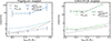 |
Fig. B.2. Connectivity of central galaxies as a function of their stellar mass in the Flagship (model m3) and GAEA (model ECLH) mocks, right and left panels, respectively, for M*-limited samples ( |

Figure B.3 shows the mean multiplicity of central galaxies as a function of their stellar mass in the model m3 of Flagship (left) and model ECLH of GAEA (right) for M*-limited samples with reduced sampling and redshift uncertainties (𝒟noise, 60%) with tessellation weighting, but qualitatively similar results are found without weighting. The multiplicity appears to be a more robust quantity than the connectivity, given that the FoG effect has an overall much weaker impact on its values, in particular when the tessellation is weighted by stellar mass.
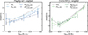 |
Fig. B.3. Multiplicity of central galaxies as a function of their stellar mass in Flagship (model m3) and GAEA (model ECLH) mocks, left and right panels, respectively, for M*-limited samples ( |

Figure B.4 shows the multiplicity of central galaxies as a function of their stellar mass for the Flagship and GAEA mocks (models m3 and ECLH, respectively, with qualitatively similar conclusions for m1 and ECLQ) for the fiducial sample (𝒟noise, 60%) without stellar mass-weighted tessellation. The multiplicity of central galaxies increases with increasing stellar mass for galaxies in all reference catalogues (𝒟), catalogues with reduced sampling and redshift uncertainties (𝒟noise, 60%). The applied FoG correction significantly improves our ability to recover the M*-multiplicity relation.
Appendix C: Stellar-mass gradients
Figure C.1 shows the PDFs of the distances of galaxies to their closest filament for the Flagship m1 model (the results for the Flagship m3 and GAEA models are comparable) and for the reconstruction of the cosmic web with weighting the tessellation as a function of stellar mass and redshift, for Hα flux-limited sample with reduced sampling (𝒟60%, first row) and when redshift error and FoG are added ( , second row). Stellar-mass gradients, with more massive galaxies located closer to the filaments than their lower mass counterparts, present in the reference Hα flux-limited sample are recovered.
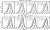 |
Fig. C.1. Same as in Fig. 14, but for a catalogue with reduced sampling (𝒟60%; top) and with added redshift error and FoG ( |

Figure C.2 shows the PDFs of the distances of galaxies to their closest filament for the Flagship m1 model (the results for the Flagship m3 and GAEA models are comparable) and for the reconstruction of the cosmic web without weighting the tessellation as a function of stellar mass and redshift. The distances are normalised by the mean intergalactic separation to take into account the effect of decreasing the density of galaxies with increasing redshift.
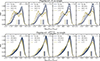 |
Fig. C.2. Same as in Fig. 14, but for the reconstruction without stellar mass-weighted Delaunay tessellation. The error on redshift in combination with the redshift-space distortions strongly reduce the stellar-mass gradients, that are only slightly improved after the correction of the FoG effect. |
The first row shows the PDFs for the reference sample (𝒟), while the second row shows the PDFs after correction of the FoG effect ( ). When the cosmic web is reconstructed without weighting the Delaunay tessellation, reduced galaxy sampling tends to decrease the stellar mass gradient signal (not shown), as in the case of the reconstruction including the weighting. Redshift errors have the strongest impact, by significantly reducing our ability to recover the stellar-mass gradients towards filaments of the cosmic web (not shown). Correcting for the FoG effect only mildly improves the signal.
All Tables
Median and mean connectivity for the Flagship m3 and Flagship m1 mocks for tessellations with and without stellar mass weighting.
Median and mean connectivity for the GAEA ECLH and GAEA ECLQ mocks for tessellations with and without stellar mass weighting.
Median and mean multiplicity for the Flagship m3 and Flagship m1 mocks for tessellations with and without stellar mass weighting.
Median and mean multiplicity for the GAEA ECLH and GAEA ECLQ mocks for tessellations with and without stellar mass weighting.
All Figures
|
Fig. 1. Mean intergalactic separation in Flagship (blue colours) and GAEA (green colours) simulations for all considered models (m1 and m3 for Flagship, ECLH and ECLQ for GAEA). For each model, the fiducial galaxy selection based on the Hα flux (Hα) is compared to the stellar mass-based selection (M*). Shaded regions correspond to the standard deviation across five mocks for each model. Dotted and dashed grey lines represent the corresponding redshift uncertainties converted into distances for Flagship and GAEA simulations, respectively. GAEA models show smaller differences between each other and compared to the Flagship simulation models, in particular for the Hα selection of galaxies. Above z ∼ 0.9, the Hα selection follows the selection more closely, based on stellar mass for the Flagship simulation, with respect to GAEA. |
| In the text | |
|
Fig. 2. Stellar mass (left) and Hα luminosity functions (right) in three redshift bins, 0.4 < z < 0.9 (top), 0.9 < z < 1.3 (middle), and 1.3 < z < 1.7 (bottom), in all models considered in this work for Hα flux limited samples (coloured solid lines) and for samples without any limit (coloured dashed lines). Black symbols correspond to observational data at these redshifts, COSMOS2020 (Shuntov et al. 2022) for stellar mass functions and the Emission Line COSMOS catalogue (Saito et al. 2020), HST-NICMOS (Shim et al. 2009), HST WISP (Colbert et al. 2013), and HiZELS (Sobral et al. 2013) for Hα luminosity functions. |
| In the text | |
|
Fig. 3. Star-forming main sequence in the Flagship (left) and GAEA (right) simulations (models m3 and ECLH, respectively) at 0.4 < z < 0.9 (top) and 0.9 < z < 1.8 (bottom), color-coded by the Hα luminosity, which essentially correlates with SFR. The red lines correspond to the compilation of observational data presented in Popesso et al. (2023). The contours encompass 50% and 75% of the galaxy distribution for Hα flux-limited sample (solid lines) and for the sample without any limit (dashed lines). |
| In the text | |
|
Fig. 4. Two-point correlation functions of galaxies in the redshift range 0.8 < z < 1.3 for galaxies with the 5% highest and lowest Hα flux in the Flagship m3 (left) and GAEA ECLH (right) mocks. Shaded regions correspond to jackknife error bars. At small separations (≲1 h−1 Mpc), brightest galaxies show enhanced clustering in Flagship compared to their low Hα flux counterparts, while the brightest galaxies in GAEA show comparable (or reduced) clustering to their lower brightness counterparts. At larger separations (≳1 h−1 Mpc), the brightest galaxies are more clustered compared to their low Hα flux counterparts in all mocks. |
| In the text | |
|
Fig. 5. Visualisation of a ∼40 h−1 Mpc thick slice of the galaxy distribution from the Flagship m3 mock and the corresponding cosmic web skeleton reconstructed without weighting Delaunay tessellation for the reference catalogue without the FoG effect, without added noise and with 100% completeness (𝒟; top), with the FoG, added redshift error and 60% sampling ( |
| In the text | |
|
Fig. 6. Same as in Fig. 5, but for the GAEA ECLH mock. The higher galaxy number density of the GAEA ECLH mock compared to Flagship m3 (Fig. 5) can be clearly seen. |
| In the text | |
|
Fig. 7. PDF of filament lengths (top), wall areas (middle) and void volumes (bottom) for Flagship mocks (model m3) without redshift-space distortions for full (𝒟; solid grey lines), and 60% (𝒟60%; solid coloured lines) sampling, including the FoG effect ( |
| In the text | |
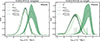 |
Fig. 8. Same as in Fig. 7, but for GAEA mocks (model ECLH) and filament lengths alone. |
| In the text | |
|
Fig. 9. PDFs of the connectivity of central galaxies for the Hα-limited selection of galaxies in the full sample without redshift error (𝒟) for Flagship model m3 (top) and GAEA model ECLH (bottom) mocks, with stellar mass weighting of the skeleton (left) and without weighting (right). In each panel, vertical lines indicate the medians of distributions. For a better visibility, the histograms are limited to the connectivity values below 14. Mean and median values for all distributions are reported in Tables B.1 and B.2. The redshift-space distortions have a strong impact on the connectivity of galaxies, but this effect that can be reasonably corrected for. |
| In the text | |
|
Fig. 10. PDFs of the connectivity of central galaxies for the Hα-limited selection of galaxies in the fiducial sample (𝒟noise, 60%; coloured lines) for Flagship model m3 (left) and GAEA model ECLH (right) mocks, with stellar mass weighting of the skeleton. The full sample without noise (𝒟) is shown for comparison (grey lines). In each panel, vertical lines indicate the medians of distributions and error bars correspond to the standard deviation across five mocks. For a better visibility, the histograms are limited to the connectivity values below 14. Mean and median values for all distributions are reported in Tables B.1 and B.2. Redshift errors and incompleteness of the sample decrease the quality of the cosmic web reconstruction, which can be improved by stellar mass weighting. |
| In the text | |
|
Fig. 11. PDFs of the multiplicity of central galaxies for an Hα-limited selection of galaxies in the fiducial sample (𝒟noise, 60%; coloured lines) for Flagship model m3 (left) and GAEA model ECLH (right) mocks, with stellar mass weighting of the skeleton. The full sample without noise (𝒟) is shown for a comparison (grey lines). In each panel, vertical lines indicate the medians of distributions and error bars correspond to the standard deviation across five mocks. The mean and median values for all distributions are reported in Tables B.3 and B.4. The multiplicity of the cosmic web shows only a weak sensitivity to the FoG effect, redshift error, and sample completeness. |
| In the text | |
|
Fig. 12. Connectivity of central galaxies as a function of their stellar mass in Flagship model m3 (top) and GAEA model ECLH (bottom) mocks for the fiducial galaxy sample 𝒟noise, 60%, with stellar mass weighting of the skeleton (left) and without weighting (right). As expected, connectivity increases with stellar mass, with weighting of the Delaunay tessellation introducing a bias at lower stellar masses leading to reversed trend. Correction for the FoG effect is needed to recover reasonably well the M*-connectivity relation, in particular for weighted tessellations. |
| In the text | |
|
Fig. 13. Multiplicity of central galaxies as a function of their stellar mass in Flagship model m3 (left) and GAEA model ECLH (right) mocks for the fiducial sample, with stellar mass weighting of the skeleton. As for connectivity, multiplicity increases with M*, with a reversed trend at low M*. In contrast to connectivity, the redshift-space distortions do not strongly modify the amplitude of the M*-multiplicity relation. |
| In the text | |
|
Fig. 14. PDFs of the closest filament’s distance, normalised by the redshift dependent mean intergalactic separation, for galaxies in the Flagship mock (model m3) in different stellar mass bins (coloured lines; with numbers indicating log10(M*/M⊙) values) and the cosmic web reconstructed using the stellar mass-weighted Delaunay tessellation. Stellar-mass gradients are shown as a function of redshift from the lowest redshift bin (left) to the highest one (right). Stellar-mass gradients, with more massive galaxies located closer to the filaments than their lower mass counterparts, present in the reference Hα flux-limited sample (𝒟; top), are recovered when the FoG correction is performed ( |
| In the text | |
|
Fig. A.1. PDF of filament lengths for Hα- (left) and stellar mass-limited (right) samples. Top and bottom panels compare non-weighted and weighted tessellations, respectively, for the Flagship m3 model. Vertical lines indicate the medians of distributions. Shaded regions correspond to the bootstrap error bars. For the stellar mass-limited galaxy sample, weighting of the Delaunay tessellation for the cosmic web reconstruction is not required to obtain a good agreement for the distribution of filaments’ length. |
| In the text | |
|
Fig. A.2. Same as in Fig. A.1 (bottom) i.e. using the stellar mass-weighted tessellation for the cosmic web reconstruction, but for the GAEA ECLH model. |
| In the text | |
|
Fig. A.3. PDF of filaments’ length for stellar mass-limited (left) and Hα-limited (right) samples with 60 % sampling. |
| In the text | |
|
Fig. B.1. Same as in Fig. 9, but for the M*-limited galaxy selection. The mean and median values for all distributions are reported in Tables B.1 and B.2. |
| In the text | |
|
Fig. B.2. Connectivity of central galaxies as a function of their stellar mass in the Flagship (model m3) and GAEA (model ECLH) mocks, right and left panels, respectively, for M*-limited samples ( |
| In the text | |
|
Fig. B.3. Multiplicity of central galaxies as a function of their stellar mass in Flagship (model m3) and GAEA (model ECLH) mocks, left and right panels, respectively, for M*-limited samples ( |
| In the text | |
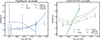 |
Fig. B.4. Same as in Fig. 13, but without any stellar mass weighting of the skeleton. |
| In the text | |
|
Fig. C.1. Same as in Fig. 14, but for a catalogue with reduced sampling (𝒟60%; top) and with added redshift error and FoG ( |
| In the text | |
|
Fig. C.2. Same as in Fig. 14, but for the reconstruction without stellar mass-weighted Delaunay tessellation. The error on redshift in combination with the redshift-space distortions strongly reduce the stellar-mass gradients, that are only slightly improved after the correction of the FoG effect. |
| In the text | |
Current usage metrics show cumulative count of Article Views (full-text article views including HTML views, PDF and ePub downloads, according to the available data) and Abstracts Views on Vision4Press platform.
Data correspond to usage on the plateform after 2015. The current usage metrics is available 48-96 hours after online publication and is updated daily on week days.
Initial download of the metrics may take a while.