| Issue |
A&A
Volume 708, April 2026
|
|
|---|---|---|
| Article Number | A312 | |
| Number of page(s) | 59 | |
| Section | Planets, planetary systems, and small bodies | |
| DOI | https://doi.org/10.1051/0004-6361/202557546 | |
| Published online | 23 April 2026 | |
Observational constraints on the chemical tracers of planet formation history
A systematic survey of 13 directly imaged low-mass companions with VLT/ERIS★
1
ETH Zurich, Institute for Particle Physics and Astrophysics,
Wolfgang-Pauli-Strasse 27,
8093
Zurich,
Switzerland
2
Max Planck Institute for Intelligent Systems,
Max-Planck-Ring 4,
72076
Tübingen,
Germany
3
National Center of Competence in Research PlanetS,
Switzerland
4
University of Zurich,
Rämistrasse 71,
8006
Zurich,
Switzerland
5
European Southern Observatory,
Alonso de Córdova 3107,
Vitacura, Santiago,
Chile
6
Max-Planck-Institut für extraterrestrische Physik,
Postfach 1312,
85741
Garching,
Germany
7
Space Sciences, Technologies, and Astrophysics Research Institute, Université de Liège,
4000
Sart Tilman,
Belgium
8
Leiden Observatory, Leiden University,
Einsteinweg 55,
2333
CC
Leiden,
The Netherlands
9
ETH Zurich, Department of Earth and Planetary Sciences,
Sonneggstrasse 5,
8092
Zurich,
Switzerland
10
Aix Marseille Université, CNRS, CNES, LAM,
Marseille,
France
11
Department of Physics & Astronomy, Johns Hopkins University,
3400 N. Charles Street,
Baltimore,
MD
21218,
USA
12
Department of Physics, University of California, Santa Barbara,
Santa Barbara,
CA
93106,
USA
13
LIRA, Observatoire de Paris, Univ PSL, CNRS, Sorbonne Univ, Univ de Paris,
5 place Jules Janssen,
92195
Meudon,
France
14
Department of Physics and Astronomy, University of Texas at San Antonio,
San Antonio,
TX
78249,
USA
15
Max-Planck-Institut für Astronomie,
Königstuhl 17,
69117
Heidelberg,
Germany
16
Laboratoire Lagrange, Université Côte d’Azur, CNRS, Observatoire de la Côte d’Azur,
06304
Nice,
France
17
INAF – Osservatorio Astrofisico di Arcetri,
Largo E. Fermi 5,
50125,
Firenze,
Italy
18
INAF – Osservatorio Astronomico di Padova,
Vicolo dell’Osservatorio 5,
35122,
Padova,
Italy
19
STFC UK ATC, Royal Observatory Edinburgh, Blackford Hill.
Edinburgh,
EH9 3HJ,
UK
20
I. Physikalisches Institut, Universität zu Köln,
Zülpicher Str. 77,
50937
Köln,
Germany
21
INAF – Osservatorio Astronomico d’Abruzzo, Via Mentore Maggini,
64100
Teramo,
Italy
★★ Corresponding author: This email address is being protected from spambots. You need JavaScript enabled to view it.
Received:
3
October
2025
Accepted:
18
February
2026
Abstract
Context. Constraining the link between the atmospheric composition of giant exoplanets and their formation history is a key goal of exoplanet studies. In particular, the atmospheric carbon-to-oxygen (C/O) ratio and metallicity – which are readily measurable with direct spectroscopic observations – are believed to be chemical tracers of the birth location of substellar and planetary companions.
Aims. We aim to collect observational constraints for planet formation theories by performing a large and systematic survey of the atmospheric C/O ratio and metallicity.
Methods. We collected new K-band moderate-resolution (R ~ 11 000) spectroscopic observations of 13 directly imaged planetary-mass companions spanning the molecular snowlines of CO2, CO, and CH4 and with masses 4–30 MJ with VLT/ERIS/SPIFFIER. Additionally, we gathered a large portion of the available archival observations for these targets, amounting to 40 spectra and 140 photometric fluxes. We performed spectral fits using self-consistent grid models and freely parametrisable models. We obtained robust estimates of the key atmospheric parameters by aggregating the results from the different models, thereby reducing modelling systematics.
Results. Using molecular mapping, we detected H2O and CO in 12 of our targets as well as 13CO in HR 2562 B. With our multimodel spectral fitting strategy, we obtained stellar to superstellar C/O ratios – ranging between 0.3 and 0.8 – and predominantly superstellar metallicities – between −1 and 1 dex – across all targets. We measured a substantial enrichment of 13CO for HR 2562 B with 12CO/13CO= 12.0−3.3+4.5. If corroborated by independent observations, it could indicate that the companion might have formed beyond the CO snowline and later migrated inwards to its current location. We find an anti-correlation (R = −0.64) between the C/O ratio and the companion mass, consolidating a previous result.
Conclusions. Our work demonstrates the scientific potential of the ERIS/SPIFFIER instrument for the orbital and atmospheric characterisation of close-in substellar and exoplanet companions.
Key words: techniques: high angular resolution / techniques: imaging spectroscopy / planets and satellites: atmospheres / planets and satellites: formation / infrared: planetary systems
Based on observations collected at the European Organisation for Astronomical Research in the Southern Hemisphere under ESO programs 112.2628.001, 112.2628.002, and 112.2628.003.
F.R.S.-FNRS Research Director.
© The Authors 2026
 Open Access article, published by EDP Sciences, under the terms of the Creative Commons Attribution License (https://creativecommons.org/licenses/by/4.0), which permits unrestricted use, distribution, and reproduction in any medium, provided the original work is properly cited.
This article is published in open access under the Subscribe to Open model. This email address is being protected from spambots. You need JavaScript enabled to view it. to support open access publication.
1 Introduction
Linking the atmospheric composition of giant exoplanets and substellar companions with their formation history has been a key goal of exoplanet studies for the past decade (Madhusudhan 2019; Feinstein et al. 2025). The original idea that the birth location of gas giants could be traced by their atmospheric composition first came from the simple remark that molecular snowlines – which denote the radial distance beyond which a gaseous molecule in the protoplanetary disc freezes into ice – would significantly influence the balance of elemental abundance ratios of volatile disc matter in the gas or solid phase (Öberg et al. 2011).
A planet forming outside of the water snowline via coreaccretion (Pollack et al. 1996) would start slowly building a core from the abundant H2O ice and other refractory elements – with its growth limited by its cooling efficiency (Lee & Chiang 2015) – until it reaches the rapid runaway gas accretion phase. At that point, it would accrete the surrounding oxygen-depleted gas until the mass of the gas becomes similar to that of the accreted solids (Mizuno 1980; Stevenson 1982; Bodenheimer et al. 2000; Rafikov 2006). The atmospheric composition of the forming planet would thus inherit the oxygen depletion of the accreted gas, leading to an increased carbon-to-oxygen (C/O) elemental abundance ratio compared to the gas contained within the H2O snowline.
On the other hand, a substellar companion forming via gravitational instability – which is believed to occur when a protoplanetary disc is massive enough to overcome its gas pressure and centrifugal forces (Kuiper 1951; Boss 1997) – would inherit the chemical composition of the disc (Feinstein et al. 2025). These theoretical considerations motivated the idea that measurements of elemental ratios – enabled by remote sensing of exoplanets (Madhusudhan 2018) – could trace the origins of exoplanet formation relative to the location of the molecular snowlines (Madhusudhan et al. 2011; Turrini et al. 2021; Mollière et al. 2022).
Countless factors and physical processes have been put forward since the elaboration of these theories that complicate the simple picture they propose and confuse the link between atmospheric composition and planet formation history (see the following reviews: Goldreich et al. 2004; Johansen & Lambrechts 2017; Mordasini & Burn 2024; Feinstein et al. 2025). For example, protoplanetary discs are shaped by the opacities and evolution of the dust (Schmitt et al. 1997; Birnstiel et al. 2016; Savvidou et al. 2020). The discs evolve over time (Lynden-Bell & Pringle 1974) through photoevaporation (Clarke et al. 2001) and disc winds (Bai et al. 2016; Suzuki et al. 2016; Chambers 2019), can be affected by instabilities (Flock et al. 2017; Klahr et al. 2018), and they can form vortices (Lobo Gomes et al. 2015) and open gaps (Lin & Papaloizou 1986; Crida et al. 2006; Pinilla et al. 2015; Binkert et al. 2021) when massive planets are forming. Beyond structural and thermal changes in protoplanetary discs (which modify the positions of the molecular snowlines), their chemical makeup is further affected by transport. Large pebbles can drift inwards through the protoplanetary disc faster than the gas, releasing volatile-rich ice when they cross their molecular snowlines and thereby change the balance between volatile and refractory elements (Cuzzi & Zahnle 2004; Öberg & Bergin 2016; Booth et al. 2017). Moreover, planets continue to accrete planetesimals after emptying their feeding zones, and the growth of the core stops (Lissauer 1987) when gas-accreting planets increase their feeding zone (Pollack et al. 1996) and migrate (Tanaka & Ida 1999; Turrini et al. 2021).
This long – yet incomplete – list of processes and factors makes it challenging to create a clear and consistent picture of the link between the atmospheric composition of substellar companions and their formation history. A promising means of disentangling the relative importance of each process is to create an inventory of the diversity of atmospheric compositions and investigate whether trends emerge from a population analysis. The atmospheric C/O ratio and metallicities have been readily measured for a range of directly-imaged (DI) substellar companions and exoplanets. To name only a few, there are estimates available for the four exoplanets in the HR 8799 system (Konopacky et al. 2016; Ruffio et al. 2021; Wang et al. 2023; Nasedkin et al. 2024), β Pic b (Gaia Collaboration 2020; Landman et al. 2024), AB Pic b (Palma-Bifani et al. 2023), and AF Lep b (Zhang et al. 2023b; Palma-Bifani et al. 2024; Balmer et al. 2025a; Denis et al. 2025). Recently proposed as an additional tracer of planet formation accessible by remote sensing (Mollière & Snellen 2019), the 13CO isotopologue has been detected in a few companions: YSES-1 b (Zhang et al. 2021a), HIP 79098 (AB) B (Xuan et al. 2024), VHS 1256 b (Gandhi et al. 2023), GQ Lup B (Xuan et al. 2024; González Picos et al. 2025), and DH Tau b (Xuan et al. 2024).
However, inhomogeneous spectral resolutions and wavelength coverages as well as different spectral fitting strategies render comparisons between studies of single targets problematic. So far, only a few studies have compared the atmospheric composition of a population of companions. Hoch et al. (2023) compared the atmospheric C/O ratios of a few DI companions – only one of which was measured in their study – with a sample of transiting planets, finding a negative trend with companion mass. Nasedkin et al. (2024) investigated a broad range of atmospheric models to fit the archival data of the HR 8799 planets, deriving a stellar to superstellar C/O ratio and metallicity. Xuan et al. (2024) applied the same spectral fitting framework to KPIC observations of eight substellar companions, finding broadly solar C/O ratios and metallicities. With the largest sample so far, Petrus et al. (2023) analysed a homogeneous sample of 43 isolated brown dwarfs and substellar companions with the X-Shooter instrument at the Very Large Telescope (VLT), comparing the results of fits obtained with the grid models Exo-REM (Baudino et al. 2015, 2017), Sonora Diamondback (Marley et al. 2021; Morley et al. 2024), and ATMO (Tremblin et al. 2016), yielding population-wide solar C/O ratios and metallicities consistent with stellar formation mechanisms. These systematic population analyses offer the best chance at constraining the link between the atmospheric composition of substellar companions and their formation history.
In that light, we performed a large (N ≥ 10) and systematic investigation of the key atmospheric tracers of giant planet formation, namely, the C/O ratio, metallicity, and 12CO/13CO isotopologue ratio. As part of the ETH Zurich Guaranteed Time Observations (GTO) program, we obtained new K-band R ~ 11 000 spectroscopic observations with the new Enhanced Resolution Imager and Spectrograph (ERIS; Davies et al. 2023), which is mounted on the Unit Telescope four at the VLT. As the most recent adaptive optics (AO) assisted, diffraction-limited infrared facility on an 8 m class telescope, ERIS offers a promising avenue to investigate the atmospheric composition of young, DI, substellar companions across the carbon-bearing molecular snowlines (CH4, CO, CO2), and maybe even within the H2O snowline (Hayoz et al. 2025). Apart from our new datasets, we also collected a large set of archival data for all of our targets, totalling 40 spectra and over 140 photometric fluxes. Armed with this wealth of data, we applied a state-of-the-art, multimodel spectral fitting strategy, combining the results of several models to obtain robust estimates of the atmospheric parameters of our targets (Nasedkin et al. 2024; Petrus et al. 2024). This enabled us to investigate trends between the C/O ratio, metallicity, and 12CO/13CO isotopologue ratio in relation to the mass of our targets and their current location relative to the molecular snowlines.
In Sect. 2, we describe our target sample (Sect. 2.1), observations (Sect. 2.2), data reduction (Sect. 2.3), and the archival data that we collected (Sect. 2.4). In Sect. 3, we introduce our spectral fitting strategy by revisiting our atmospheric retrieval framework CROCODILE (Sect. 3.1) and by describing our choice of freely parametrised models (Sect. 3.2) and self-consistent grid models (Sect. 3.3). We present our results in Sect. 4, specifically our detection of our observed companions in the molecular maps of H2O, CO, and – for one target – even 13CO (Sect. 4.1). In the appendix, we characterise their orbit by measuring their relative astrometry (Appendix I.1) and Radial Velocity (RV) (Appendix I.2). We present the results of our spectral fits in Sect. 4.2. In Sect. 5, we compare our estimated atmospheric parameters with previous studies (Sect. 5.1), investigate the robustness of our retrieved molecular abundances (Sect. 5.2), highlight the signs of chemical disequilibrium in the atmospheres of our targets (Sect. 5.3), and constrain their 12CO/13CO isotopologue ratio (Sect. 5.4). We discuss the different formation scenarios that are compatible with our retrieved atmospheric properties for each of our targets (Sect. 5.5) and how our population analysis helps constrain the link between the atmospheric composition and the formation history of substellar companions (Sect. 5.6). As we present the first High-Contrast Imaging (HCI) observing campaign with ERIS/SPIFFIER, we discuss the lessons learned, best observing practices, and future work required to further improve the scientific return of the new instrument for DI companions (Sect. 5.7). In Sect. 6, we summarise our key results and provide concluding remarks.
2 Observations
2.1 Description of the sample
We selected a sample of DI substellar companions spanning the molecular snowlines of CO2, CO, and CH4 within the reach of the capabilities of the ERIS/SPIFFIER instrument. We started by downloading the list of DI low-mass companions in the NASA exoplanet archive. We removed all targets that were not observable during the selected observing period for our GTO program, i.e. P112, as well as the targets known to be embedded in a dusty environment in order to avoid significant extinction that would prohibit molecular mapping (e.g. the PDS 70 system, Cugno et al. 2021).
Next, we determined which targets were within reach of the capabilities of the ERIS/SPIFFIER instrument. As the sensitivity limits and high-contrast capabilities of ERIS/SPIFFIER were not known at the time, we assumed that the instrument would be better than its predecessor, SINFONI, thanks to its improved Strehl ratio (Davies et al. 2023). With a Strehl ratio ~3.5 times higher for ERIS compared to SINFONI – which has been reported to be ~20% (Hoeijmakers et al. 2018; Petrus et al. 2021) – , we estimated that the detection limits of ERIS/SPIFFIER should be deeper than those of SINFONI by a factor of 3.52, i.e. ~12. We therefore removed all targets with a contrast and apparent magnitude more than 2.7 mag fainter than those of β Pic b and HIP 65426 b.
The saturation limits of ERIS/SPIFFIER prevent direct observation of bright stars, even when using its smallest field of view (FOV) – having the highest saturation limits. The only way to circumvent this restriction and avoid any detector saturation – leading to a persistent signal that might impact subsequent observations – is to offset the star outside of the FOV. This decreases the intensity of stellar light reaching the detector. However, this strategy increases the complexity of the data reduction due to the lack of robust reference for alignment of the images. Combined with pointing drifts due to residual instrument flexures, this restricts the targets to those that can be detected within a limited number of detector integrations. This effectively provides an additional sensitivity limit for exoplanets around bright stars where such off-axis observations are necessary. Concretely, these considerations can be formulated as the following two criteria for the observability of DI planets around bright stars: (i) the companions and their host stars should fit within one of the three fields of view (FoVs) of SPIFFIER whilst avoiding saturation, or (ii) be bright enough themselves to be detectable within the time it takes for the pointing drift to reach 1 λ/D (where λ is the wavelength and D the aperture size of the telescope, i.e. 1 λ/D = 58.5 mas in the K-long grating of ERIS/SPIFFIER) whilst keeping the host star outside of the FOV. At the time of preparing the sample, we assumed a pessimistic drift that would offset the target by 1 λ/D within 20 min. Since then, Hayoz et al. (2025) measured a drift timescale of 1 h. With a minimal detector integration time (DIT) of 1.6 s, the brightest stars that can be observed using the K-long grating of ERIS/SPIFFIER without exceeding half of the full well depth have a K-band magnitude of 1.6 mag1. However, this comes at the cost of significant detector overheads (see Sect. 5.7.1 for a discussion on instrument overheads), and therefore we decided to set the minimal DIT to 10 s. This effectively sets the brightness limit at K = 3.6 mag. Any targets failing to satisfy one of the above-mentioned criteria cannot be reliably observed with ERIS/SPIFFIER, and we removed them from our sample, for example β Pic with K = 3.48 mag.
The final step of our sample selection was to locate the remaining targets in relation to the molecular snowlines. For simplicity, we assumed that the locations of the molecular snowlines only depend on the stellar irradiation, and we relied on the separations calculated by Öberg et al. (2011) for the snowlines of H2O, CO2, CO, and CH4. We calculated the stellar irradiation Iirr for each of the remaining targets as well as for the molecular snowlines by using the relation ![Mathematical equation: $\[I_{\mathrm{irr}}=\frac{L_{\star}}{4 \pi a^{2}}\]$](/articles/aa/full_html/2026/04/aa57546-25/aa57546-25-eq2.png) , where L⋆ is the stellar luminosity and a is the orbital separation, which we replaced by the projected separation (i.e. ρd, with the angular separation ρ and distance from the Sun d) if the semi-major axis was unknown. The remaining targets spanned the snowlines of CO2, CO, and CH4, with the majority at large separations. We selected all remaining targets within the CH4 snowline, yielding two companions for each interval of two snowlines, as well as four companions outside of the CH4 snowline, adding to a total of ten targets and a list of backup targets. In total, 13 targets were observed over the course of three GTO observing runs, namely (in order of increasing companion mass) AF Lep b, HR 8799 e, HR 8799 c, 1RXS J160929.1-210524 b (from here on ‘1RXSJ1609 b’), ROXs 42 B b, AB Pic b, HR 2562 B, 2MASS J02192210-3925225 b (from here on ‘2MJ0219 b’), VHS J125601.92-125723.9 b (from here on ‘VHS 1256 b’), CT Cha b, ROXs 12 b, HIP 78530 B, and HIP 79098 (AB) B. We collected their currently known properties from previous studies in Tables A.1 and A.2, and we provide a summary of the current state of knowledge for each system in our sample in Appendix A. We show the companion masses derived in the literature and the stellar irradiation of our targets in Fig. 1, together with the approximate locations of the molecular snowlines. This scatter plot already highlights a selection bias of our study, namely the masses and stellar irradiations seem tightly packed into two groups. However, this is due to the properties of the currently known population of low-mass substellar companions that are within the capability of ERIS/SPIFFIER. Thus, it was not possible to avoid. Because our selection was focused on the stellar irradiation, it resulted in a list of spectrally diverse objects, as can be noticed from their position along the L branch down to the L–T transition in the J–K Hertzsprung–Russel diagram (see Fig. 2).
, where L⋆ is the stellar luminosity and a is the orbital separation, which we replaced by the projected separation (i.e. ρd, with the angular separation ρ and distance from the Sun d) if the semi-major axis was unknown. The remaining targets spanned the snowlines of CO2, CO, and CH4, with the majority at large separations. We selected all remaining targets within the CH4 snowline, yielding two companions for each interval of two snowlines, as well as four companions outside of the CH4 snowline, adding to a total of ten targets and a list of backup targets. In total, 13 targets were observed over the course of three GTO observing runs, namely (in order of increasing companion mass) AF Lep b, HR 8799 e, HR 8799 c, 1RXS J160929.1-210524 b (from here on ‘1RXSJ1609 b’), ROXs 42 B b, AB Pic b, HR 2562 B, 2MASS J02192210-3925225 b (from here on ‘2MJ0219 b’), VHS J125601.92-125723.9 b (from here on ‘VHS 1256 b’), CT Cha b, ROXs 12 b, HIP 78530 B, and HIP 79098 (AB) B. We collected their currently known properties from previous studies in Tables A.1 and A.2, and we provide a summary of the current state of knowledge for each system in our sample in Appendix A. We show the companion masses derived in the literature and the stellar irradiation of our targets in Fig. 1, together with the approximate locations of the molecular snowlines. This scatter plot already highlights a selection bias of our study, namely the masses and stellar irradiations seem tightly packed into two groups. However, this is due to the properties of the currently known population of low-mass substellar companions that are within the capability of ERIS/SPIFFIER. Thus, it was not possible to avoid. Because our selection was focused on the stellar irradiation, it resulted in a list of spectrally diverse objects, as can be noticed from their position along the L branch down to the L–T transition in the J–K Hertzsprung–Russel diagram (see Fig. 2).
 |
Fig. 1 Scatter plot of the companion masses versus stellar irradiations for our sample of 13 DI low-mass substellar companions. The dotted vertical bars indicate the rough positions of the molecular snowlines, assuming that they only depend on the stellar irradiation. The horizontal grey line shows the Deuterium Burning limit of 13 MJ that separates the brown dwarfs from the exoplanets (Spiegel et al. 2011). From left to right are AF Lep b, HR 8799 e, HR 2562 B, HR 8799 c, HIP 79098 (AB) B, HIP 78530 B, AB Pic b, 1RXSJ1609 b, ROXs 42 B b, ROXs 12 b, VHS 1256 b, 2MJ0219 b, and CT Cha b. The colours match the results presented below. |
 |
Fig. 2 Infrared Hertzsprung–Russel diagram of our sample of 13 targets (orange dots) among the population of field dwarfs (colourful dots) and young and low-gravity objects (grey squares). For reference, we also show a blackbody model (grey line) as well as the AMES-Cond model (blue line) and the AMES-Dusty model (orange line) for the ages of 20 (dotted lines) and 100 Myr (solid lines). |
2.2 ERIS/SPIFFIER observations
Our survey was carried out with ERIS-SPIFFIER in Visitor Mode during the ESO observing period P112 in the nights of 15 October and 7 November 2023 as well as 13 to 15 February 2024. The observations were taken in field-tracking mode with position angle set to 0° with the K-long grating (2.19–2.47 μm) at R ~ 11 000. We summarise the instrument setup and observing conditions in Table B.1 in Appendix B. Over the survey, we used the three available image scales (i.e. ![Mathematical equation: $\[0^{\prime\prime}_\cdot8 \times 0^{\prime\prime}_\cdot8, 3^{\prime\prime}_\cdot2 \times 3^{\prime\prime}_\cdot2\]$](/articles/aa/full_html/2026/04/aa57546-25/aa57546-25-eq3.png) , and 8″ × 8″) depending on the angular separation of the companion and apparent brightness of the host star. Concretely, we selected the largest FOV that includes both the companion and the star without reaching more than half of the full well on the brightest pixel and with a DIT greater or equal to 10 s. For targets where this was not possible, we selected the largest FOV that allowed to keep the primary star outside of the frame. The DITs were calculated using the ETC of ERIS to reach at most a third of the full well on the brightest pixel while staying under 60 sec to mitigate the effect of pointing drift caused by the residual instrument flexures. During each observation, we used a square jitter pattern of width equal to 3 px to mitigate the effect of bad pixels.
, and 8″ × 8″) depending on the angular separation of the companion and apparent brightness of the host star. Concretely, we selected the largest FOV that includes both the companion and the star without reaching more than half of the full well on the brightest pixel and with a DIT greater or equal to 10 s. For targets where this was not possible, we selected the largest FOV that allowed to keep the primary star outside of the frame. The DITs were calculated using the ETC of ERIS to reach at most a third of the full well on the brightest pixel while staying under 60 sec to mitigate the effect of pointing drift caused by the residual instrument flexures. During each observation, we used a square jitter pattern of width equal to 3 px to mitigate the effect of bad pixels.
2.3 Data reduction
The data were calibrated using our custom tool SpyFFIER2, a Python wrapper that runs the EsoRex ERIS-SPIFFIER pipeline recipes v1.6.0 (Wiezorrek et al. 2024) and that was inspired by pycrires (Stolker & Landman 2023). SpyFFIER also contains custom tools that implement the improved wavelength calibration described in Hayoz et al. (2025). The data were further post-processed using our custom package PynPoint-IFS3, a Python tool that builds upon PynPoint (Amara & Quanz 2012; Stolker et al. 2019) to enable the processing of IFS data and the computation of molecular maps. In the following, we use the words datacube, frame, and exposure interchangeably to describe one cycle of NDIT×DIT, where NDIT is the number of co-added DIT within one saved exposure. Each datacube is composed of ~ 2000 λ-images, which measure the image intensity within one wavelength channel. A slitlet describes a horizontal strip of data as sliced by one segment of the slicer mirror. We use the word spaxel to describe the spectrum extracted from a datacube at a specific spatial pixel. Finally, we use the notation X and Y for the two spatial dimensions, Λ for the spectral dimension, and T for the time dimension, as introduced by Hayoz et al. (2025).
Following Hayoz et al. (2025), our pipeline consists of dark subtraction, detector linearity, distortion correction, flat fielding, wavelength calibration, bad pixel correction, cube building, frame cropping, outlier imputation, frame selection, background subtraction, point spread function (PSF) subtraction, frame alignment, frame combination, spectrum extraction, and finally molecular mapping. As mentioned in Sect. 2.2, we used different FoVs depending on the brightness of the host star and angular separation of the companion. From the perspective of data reduction, this observing strategy resulted in three types of datasets, each requiring its own dedicated pipeline: (i) close-in targets with the star in the FOV (i.e. HR 8799 e and AF Lep b), (ii) close-in targets with the star outside of the FOV (i.e. HR 8799 c and HR 2562 B), and (iii) well-separated targets with negligible contribution from the stellar PSF at the position of the companion (i.e. all of our other targets). Whereas datasets of type (i) can be reduced with the same pipeline as described in Hayoz et al. (2025), there are two main challenges for the second type of datasets, namely the wavelength calibration and the frame alignment. Indeed, since the star is just outside of the FOV, the stellar PSF that is visible everywhere in the FOV is quite faint. Therefore, the telluric absorption lines, which imprint the stellar PSF, have a low signal-to-noise ratio (S/N) and cannot be fit very accurately. This prevents the spline fitting strategy – both along the wavelength direction and across the detector as described in Hayoz et al. (2025) – and calls for a simpler, less accurate, calibration. For the frame alignment, the problem consists in the lack of reference point relative to which the frames can be aligned. The part of the stellar PSF that is visible in the FOV is too faint to reliably use as reference with which to cross-correlate the frames. The only reference point is the companion itself, but it is hidden by the stellar PSF. Fortunately, HR 2562 B and HR 8799 c are both bright enough that we can detect them in molecular maps consisting of single frames. Therefore, we first subtracted the stellar PSF using Spectral Principal Component Analysis (PCA) (Hayoz et al. 2025), then calculated molecular maps for each frame, and recorded the position of the companion in the frames in which it was detected. The frames in which the companion cannot be detected in this way were removed, as the frame alignment could not be determined. The frames could subsequently be aligned and combined using the relative positions of the companion. The third type of datasets differ from the first two by the significantly lower proportion of the FOV that is dominated by the stellar PSF – if it is visible at all. The wavelength calibration therefore requires leveraging the OH sky emission lines rather than the telluric absorption lines imprinted in the stellar PSF (the sky emission lines are visible in the bottom row of Fig. D.2).
In Appendix D, we describe the main steps of our custom pipeline that diverge from Hayoz et al. (2025) and that we implemented to overcome the challenges posed by the three types of datasets, namely the wavelength calibration, frame alignment, background subtraction, PSF subtraction, spectrum extraction, and flux calibration. Our pipeline is summarised in the schematic depicted in Fig. D.1 in Appendix D. The major steps of our pipeline are illustrated in Fig. D.2 for our observations of HR 8799 e and 2MJ0219 b (types (i) and (iii), respectively). Our final, fully calibrated ERIS/SPIFFIER spectra are shown in Fig. 3. As we explain in Appendix D, our observations were not sensitive enough for 1RXSJ1609 b, for which the extracted spectrum has such a low S/N that the telluric absorption lines can barely be seen by eye. As we describe in Sect. 4.1, we did not detect either H2O or CO (see Fig. H.1), and therefore we chose to remove it from our sample for the remaining of our analysis.
We note here that the same stray light as described in Hayoz et al. (2025) for the AF Lep b dataset also appears in the HR 8799 e dataset, for which the star is also in the FOV. We cannot see any stray light in any of the other datasets (see Fig. D.2). It therefore seems to be visible only when a large amount of light emitted by a bright source in the FOV of ERIS-SPIFFIER, as coming from the bright stars AF Lep and HR 8799, directly enters the instrument. However, some amount of stray light might still be present in our other datasets, albeit hidden under the sky and instrument background. Future work should aim at characterising this stray light in order to remove it, as it can be a limiting factor for the detection of faint targets.
2.4 Archival data
Since our ERIS-SPIFFIER data only covers a very narrow wavelength range (2.19–2.47 μm), we cannot constrain (or only weakly constrain) many of the atmospheric parameters – such as the pressure–temperature (p–T) profile or any of the molecules without any spectral signatures in the K band – without further spectral coverage. Although we expect to be able to constrain the abundance of CO and H2O due to their strong signal in the K band, these might be degenerate with other parameters.
Therefore, we performed an extensive literature research to gather as many photometric and spectroscopic datasets as possible for our targets. We collected more than 40 spectra and over 140 photometric measurements, including yet unpublished photometric and spectroscopic data of ROXs 42 Bb (see Appendix E.1 for further details). The full list with corresponding references is given in Tables E.2 and E.1 for the photometry and spectroscopy. Following Nasedkin et al. (2024) and in agreement with all authors, we make all data used in this paper publicly available for download on Vizier and Zenodo (cf. data availability in Sect. 6).
A large number of the archival spectroscopic datasets that we gathered have a moderately high spectral resolution, i.e. R ≥ 1000. This poses a challenge for atmospheric retrievals, as the computation time of a single spectrum grows linearly with the number of wavelength channels considered (see e.g. the implementation of the radiative transfer in petitRADTRANS Mollière et al. 2019). Therefore, we have downsampled all spectroscopic datasets which have a spectral resolution greater than 1000 to a resolution of 500. Because downsampling mainly preserves the broad absorption bands and removes the narrow absorption lines, we cannot include other cross-correlation spectroscopic datasets with a large spectral resolution, such as the H-band VLT/HiRISE spectrum of AF Lep b from Denis et al. (2025).
For some datasets, the data were not (or inaccurately) absolute flux calibrated, i.e. they were normalised in some way by the authors. We performed their absolute flux calibration (in the sense described in Appendix D.5) by considering all archival photometric data available within the wavelength intervals of each spectrum. The uncertainty of each spectrum was then adjusted by the uncertainty of the photometry used for the absolute flux calibration, i.e. we estimated the uncertainty after flux calibration as ![Mathematical equation: $\[\sigma^{\prime}=\sqrt{\sigma_{\mathrm{F}}^{2}+\sigma_{\mathrm{P}}^{2}}\]$](/articles/aa/full_html/2026/04/aa57546-25/aa57546-25-eq4.png) , where σF is the uncertainty of the flux before flux calibration, and σP is the uncertainty of the photometric data. We performed the absolute flux calibration for the following datasets: the JHK-band SINFONI (Bonnefoy et al. 2014; Palma-Bifani et al. 2023) and L-band MagAO/Clio (Stone et al. 2016) spectra of AB Pic b, the YJHK-band GNIRS spectrum of HIP 78530 B (Lachapelle et al. 2015), the JHK-band SINFONI spectrum of CT Cha b (Bonnefoy et al. 2014), the YJHK-band FIRE spectrum of 2MJ0219 b (Artigau et al. 2015), the JHK-band OSIRIS and J-band NIFS spectra of ROXs 12 b (Bowler et al. 2017), the K-band SINFONI spectrum of ROXs 42 Bb (Currie et al. 2014c), the H-band GPI spectrum of HR 2562 B (Godoy et al. 2024), and the H-band GPI spectrum of HR 8799 c (Nasedkin et al. 2024).
, where σF is the uncertainty of the flux before flux calibration, and σP is the uncertainty of the photometric data. We performed the absolute flux calibration for the following datasets: the JHK-band SINFONI (Bonnefoy et al. 2014; Palma-Bifani et al. 2023) and L-band MagAO/Clio (Stone et al. 2016) spectra of AB Pic b, the YJHK-band GNIRS spectrum of HIP 78530 B (Lachapelle et al. 2015), the JHK-band SINFONI spectrum of CT Cha b (Bonnefoy et al. 2014), the YJHK-band FIRE spectrum of 2MJ0219 b (Artigau et al. 2015), the JHK-band OSIRIS and J-band NIFS spectra of ROXs 12 b (Bowler et al. 2017), the K-band SINFONI spectrum of ROXs 42 Bb (Currie et al. 2014c), the H-band GPI spectrum of HR 2562 B (Godoy et al. 2024), and the H-band GPI spectrum of HR 8799 c (Nasedkin et al. 2024).
Finally, some of our targets are affected by extinction (see the non-empty rows A0 in Table A.1 and A.2). For these, we de-reddened all the archival data using the package dust_extinction (Gordon 2024) and the G23 model applicable to Milky Way interstellar extinction.
 |
Fig. 3 Final continuum-removed, wavelength-calibrated ERIS/SPIFFIER spectra delivered by our pipeline for each of the companions observed within our survey. The spectra of each target are shown over two lines (upper and lower panels) for better readability. The typical (i.e. median) uncertainties of our measurements are indicated as an error bar on the left side of each spectrum. We show three spectral templates as reference for the features visible in the data (black), namely a telluric, H2O, and CO template. For instance, the CO lines between 2.294 μm and 2.34 μm are clearly recognisable in all spectra, whilst the H2O lines, which are distributed everywhere, are harder to identify. Due to the correction of the telluric absorption lines, some artefacts of the outlier imputation are visible at longer wavelength (in particular at 2.436 μm and 2.452 μm). We note that the spectra were transformed to the rest frame of the companions to align the spectral signatures present in the spectra, as otherwise the peculiar RVs of each companion would render this plot harder to read. |
3 Methods
The aim of this work is the robust measurement of the atmospheric C/O ratio of our ERIS/SPIFFIER survey of low-mass brown dwarfs and gas giant exoplanets. This is a challenging task, as there exist many different atmospheric models that take into account different physical processes and that can fit the Spectral Energy Distributions (SEDs) of such objects relatively well whilst resulting in different atmospheric parameters, as was demonstrated by Petrus et al. (2024) using a 1–18 μm James Webb Space Telescope (JWST) spectrum of VHS 1256 b. In that context, the emerging best practice is to compare the results of several models and propagate the uncertainties due to the different answers obtained by each model into a final, aggregated value (see e.g. Petrus et al. 2024; Nasedkin et al. 2024). Globally, there are two categories of 1D radiative models that are widely used to investigate the atmospheric properties of substellar objects (Madhusudhan 2018): (1) physically self-consistent, usually computationally expensive models that are available publicly as grids and that are calculated for a low-dimensional (2–5 dimensions) parameter space, and (2) so-called atmospheric retrievals, which are freely parametrisable models that calculate the spectra based on a high-dimensional (≥10 dimensions) prescription for the p–T profile, chemistry, and clouds. To reach our goal, we adopted a dual fitting strategy: we used multiple models of both categories to fit the spectra and retrieve the atmospheric properties of the companions. That way, if the results between the different models were severely inconsistent, we would know that the retrieved properties might not be reliable and the results should be interpreted with caution. On the other hand, if the retrieved properties agree relatively well across multiple models, then we can aggregate the different values into a final, reliable estimate which we can keep for further interpretation.
In Sect. 3.1, we revisit and update the CROCODILE framework, which required an absolute flux calibration of the spectra, to extend it to non-flux-calibrated data. In Sects. 3.2 and 3.3, we describe the parametrised forward models and the self-consistent models, respectively, that we used to fit the atmospheric parameters of our observed companions.
3.1 CROCODILE revisited
CROCODILE combines cross-correlation spectroscopy together with photometry and regular spectroscopy into the framework of atmospheric retrievals by defining a corresponding log-likelihood function for each type of data and taking the sum as the likelihood associated with the combined data (Hayoz et al. 2023). The choice of likelihood function associated with cross-correlation spectroscopy is based on Brogi & Line (2019) and was validated by Hayoz et al. (2023) in their simulation framework. However, it uses an implicit assumption that is not satisfied by our ERIS/SPIFFIER data, namely the absolute calibration of the flux. Therefore, we modified it, going back to the original formula derived by Zucker (2003) instead. We include a full derivation of the mathematical framework of CROCODILE, as well as its updated formulation, in Appendix C, where we also verify its validity.
3.2 Free atmospheric retrievals
In the following, we describe the forward models used for our free retrievals, i.e. where the atmospheric properties are parametrised and freely retrieved instead of being selfconsistently computed from macroscopic parameters. For this, we used petitRADTRANS v2.7.6 as implemented in CROCODILE. The sampling of the parameter space in CROCODILE was executed using the widely used package pymultinest (Buchner et al. 2014), which brings the multimodal nested sampling (Skilling 2006) algorithm MultiNest (Feroz et al. 2009, 2019) to Python. Due to the high computing costs of atmospheric retrievals and the large number of targets, we did not investigate all forward models proposed in the literature. Instead, we selected two models: one with free chemistry, and one with chemical equilibrium.
The first model describes the molecular abundances as vertically constant profiles parametrised by their mass fractions Xi, as is widely used in the community (see e.g. Konrad et al. 2023, 2024; Alei et al. 2024; Kühnle et al. 2025; Nasedkin et al. 2024). We included the following molecules: H2O, CO, CH4, CO2, FeH, HCN, TiO, VO, H2S. We included the isotopologue 13C16O as an additional parameter for a separate retrieval when investigating its presence and abundance in the atmosphere of our targets. Finally, we included Rayleigh scattering by molecular hydrogen and helium, as well as the collision-induced absorption (CIA) cross-sections of H2–H2 and H2–He. The list of opacity databases used in this work is given in Table G.1 in Appendix G. The atmosphere was modelled as a discrete grid of 100 layers between the pressures of 10−6 and 103 bar.
The chemical equilibrium model is the one implemented in easyCHEM (Mollière et al. 2015, 2017). It is parametrised by the elemental C/O ratio, the metallicity [Fe/H], and a quench pressure for H2O, CO, and CH4 that controls chemical disequilibrium (e.g. induced by vertical mixing). Concretely, the model assumes vertically constant C/O ratio and metallicity and calculates the chemical composition of each layer of the atmosphere given its temperature and pressure by minimising the Gibbs free energy, except at lower pressures than the quench pressure where the abundances of H2O, CO, and CH4 are maintained at the same values as that of the quench pressure. For that model, we additionally included NH3, PH3, K, and Na beyond the molecules used in our free model.
For the p–T profile, we used the Guillot analytical model (Guillot 2010):
![Mathematical equation: $\[T=\frac{3}{4} T_{\mathrm{int}}^4\left(\frac{2}{3}+\tau\right)+\sqrt{3} T_{\mathrm{equ}}^4\left(\frac{2}{\sqrt{3}}+\frac{1}{\gamma}+\left(\gamma-\frac{1}{\gamma}\right) e^{-\sqrt{3} \gamma \tau}\right),\]$](/articles/aa/full_html/2026/04/aa57546-25/aa57546-25-eq5.png) (1)
(1)
where Tequ is the equilibrium temperature of an irradiated body, Tint is the intrinsic temperature of the planet, γ is the ratio between the mean opacity in the optical and infrared range, and the optical depth is given by τ = κIRP/g where P is the pressure, g the surface gravity, and κIR is the mean opacity in the infrared range. These parameters have physically motivated meanings, as they describe an irradiated atmosphere with internal heat from below (Guillot 2010). However, we simply used this model as a parametrisation of the p–T profile, similarly as in Nasedkin et al. (2024). For the treatment of the clouds, we considered a clear atmosphere in the free chemistry model, whereas we included a clear version and a cloudy version for the chemical equilibrium model. Our cloud model is given by the simple grey cloud deck implemented in petitRADTRANS. It is parametrised by a cloud pressure below which the opacities at all wavelengths are set to infinity. The remaining variables of the model are the radius of the planet RP and the distance to the stellar system d, where RP is a free parameter of the model whilst d was set to the value measured by GAIA. In summary, our free model has 16 parameters: nine for the molecular abundances, five for the p–T profile, one for the planetary radius, and one for the cloud deck. On the other hand, our chemical disequilibrium model has ten parameters. We used the priors listed in Table 1.
Priors used for our free retrievals.
3.3 Self-consistent models
Along with the free models described in Sect. 3.2, we also investigated the parameters derived by self-consistent model grids, namely Sonora-Diamondback, Exo-REM, and BT-Settl CIFIST models. Sonora-Diamondback is a 1D radiative-convective equilibrium model describing the evolution of the atmospheres of substellar objects and their spectra, covering the L, T, and Y spectral types (Marley et al. 2021), with a recently implemented treatment of clouds (Morley et al. 2024). The exoplanet radiative-convective equilibrium model (Exo-REM, Baudino et al. 2015, 2017) is a 1D radiative-convective equilibrium model for exoplanets and brown dwarfs that successfully reproduces the L and T spectral types as a function of effective temperature thanks to its treatment of clouds, which is based on the Ackerman-Marley model based on the diffusion and sedimentation of condensates (Ackerman & Marley 2001). Finally, the BT-Settl CIFIST model (Allard et al. 2012) computes the abundance and size distributions of dust grains in the atmospheres of low-mass stars down to planetary objects under the assumption of solar chemical abundances (Caffau et al. 2011), and it calculates their spectra using the PHOENIX code (Hauschildt et al. 1997; Allard et al. 2001). We used the python package species (Stolker et al. 2020) to download and fit the above-mentioned grid models to the data, and we used pymultinest (Buchner et al. 2014; Feroz et al. 2009, 2019) for the parameter sampling. The bounds and step sizes of the grid models are given in Table 2. In addition to the parameters described in this table, species also fits for the planetary radius and parallax of the stellar system, for which it assumes a normal distribution with mean and standard deviation equal to the measurement by GAIA. For the sake of clarity, we explicitly give the number of parameters included in each model in Table 3.
Unfortunately, some of our targets have effective temperatures that fall outside of the prior bounds of one or more of the self-consistent models selected for this study. Fitting a spectrum with the wrong model can lead to biased estimates of the atmospheric parameters. Therefore, we used prior knowledge of the spectral types and effective temperatures of our targets (see Tables A.1 and A.2) to identify which models do not apply to which targets. For Sonora-Diamondback, AF Lep b is thought to be colder than 900 K, whilst CT Cha b, ROXs 12 b, and HIP 78530 B might be too hot, with Teff estimates that are overlapping with the bound of the model (i.e. Teff ≥ 2400 K). For Exo-REM, ROXs 42 B b, CT Cha b, ROXs 12 b, HIP 78530 B, and HIP 79098 (AB) B are hotter than 2000 K. Finally, AF Lep b, HR 8799 c, HR 8799 e, and VHS 1256 b are believed to be colder than 1200 K, and therefore too cold for BT Settl CIFIST.
Model bounds and step size used for our self-consistent grid retrievals.
4 Results
In Sect. 4.1, we compute molecular maps (Hoeijmakers et al. 2018; Hayoz et al. 2025) of the targeted systems. In Sect. 4.2, we investigate their atmospheric properties.
4.1 Molecular maps
As shown in our previous work (Hayoz et al. 2025), molecular mapping with ERIS/SPIFFIER allows to search for substellar companions as close as 100 mas to a star by effectively suppressing speckles using PSF subtraction with spectral PCA and picking up on the spectral signatures of specific molecules. Additionally, molecular mapping provides a robust technique to investigate the presence of trace gases in the atmosphere of substellar companions (see e.g. Hoeijmakers et al. 2018; Mâlin et al. 2023; Hayoz et al. 2025). Beyond these two molecules, the K-long grating offers access to the spectral signature of the isotopologue 13C16O, the abundance of which is hypothesised to trace the relative location of the formation of the companion with respect to the CO snowline (Zhang et al. 2021a,b). For these reasons, we computed molecular maps for all of our targets.
After PSF subtraction with spectral PCA or high-pass filtering as described in Appendix D.4, we aligned and median-combined the datacubes of each observation, resulting in one master cube for each target and each night of observation. For close-in targets, we additionally convolved the data with an aperture of radius 1.7 px as in Hayoz et al. (2025) to gather more signal coming from the companions and thereby increasing the S/N of their spectra. We subsequently computed molecular maps with spectral templates for the following molecules which all contain opacity lines in the K band: H2O, CO, 13C16O, CH4, CO2, H2S, NH3, and HCN. We followed the methods described in Hayoz et al. (2025) to compute molecular maps, i.e. by plotting the cross-correlation coefficient at the RV of the companion and assessing the significance of the detection by comparing the peak of the cross-correlation function to the distribution of values at the same RV in the rest of the image.
The resulting molecular maps of our HCI targets are shown in Fig. 4 along with the image intensity (i.e. the datacube averaged over the wavelength axis) and cross-correlation functions with the extracted spectrum, whilst the molecular maps for the rest of our targets are shown in Figs. H.1 and H.2 in Appendix H. For the well-separated targets, all the companions were easily detected in the intensity images, whereas the close-in companions (AF Lep b, HR 8799 e, HR 8799 c, and HR 2562 B) were only revealed in the molecular maps. We robustly detected all of our targets in the molecular maps of H2O and CO with the exception of 1RXSJ1609 b, which was only detected in the intensity image. The non-detection of H2O and CO in the atmosphere of 1RXSJ1609 b is probably due to a low S/N. Indeed, the telluric lines were barely visible by eye in single frame spectra of the companion, leading to complications in the telluric correction and spectrum extraction (see Appendix D.5). With frames of DIT=30 s and a total integration time of 18 min, this is probably too short for this faint target. We therefore left this target out of our analysis in the rest of this paper, except for the measurement of the relative astrometry in Appendix I.1.
The CO bandhead and ‘forest’ at λ ≳ 2.293 μm can be seen very clearly in some of the objects in Fig. 3. However, it is hard to recognise H2O because of its lack of strong spectral features. We provide a side-by-side comparison of our ERIS/SPIFFIER spectra with our best-fit model in Figures J.1–J.12, in which the quality of our data is made clearer.
We report the robust detection of the isotopologue 13C16O in the atmosphere of HR 2562 B (see Fig. 5), but not in any other of our targets. We investigate the abundance of 13C16O in the atmosphere of our targets in Sect. 5.4. The detection of the isotopologue only in HR 2562 B can be attributed to the differences in S/N of our spectra. Indeed, our observation of HR 2562 B resulted in the spectrum with the highest S/N out of our sample (see the size of the error bars in Fig. 3). This can be explained by both a relatively long integration time for such a bright target and an accurate PSF subtraction.
The detection of 13C16O only in HR 2562 B and not in comparably warm companions such as VHS 1256 b might also be the consequence of differences in cloud structure and the atmospheric depths probed (e.g. Ackerman & Marley 2001; Marley et al. 2010; Vos et al. 2020) rather than differences in chemical equilibrium (Burrows & Sharp 1999; Lodders & Fegley 2002). Although the CO-dominated region shifts towards higher altitude with increasing effective temperature (Visscher & Moses 2011), the observability of optically thin isotopologues such as 13C16O is primarily controlled by cloud opacity (Marley et al. 2010; Zahnle & Marley 2014). In clear atmospheres or when sedimentation is high, deeper CO-rich layers become accessible, enhancing the detectability of the weak features of its isotopologues (Ackerman & Marley 2001; Saumon et al. 2006). Conversely, the vertically extended cloud decks of young, low-gravity objects can obscure these CO-rich layers, effectively suppressing the signature of 13C16O even when it is predicted by equilibrium chemistry (Apai et al. 2013; Biller et al. 2015; Miles et al. 2020). This interpretation is consistent with the atmospheric properties of both HR 2562 B and VHS 1256 b. Indeed, HR 2562 B lies at the end of the L/T transition and exhibits a largely cloud-free atmosphere (Godoy et al. 2024). On the other hand, VHS 1256 b resides at the beginning of the L/T transition and displays strong variability, patchy cloud coverage, and significant dust content (Gauza et al. 2015; Miles et al. 2020; Zhou et al. 2020; Miles et al. 2023). Despite similar effective temperatures and masses, the substantial age difference between these objects implies different sedimentation efficiencies and cloud vertical structures. In our sample, HR 2562 B is the oldest object, for which the detection of 13C16O is more favourable given the advanced sedimentation of condensates in the atmosphere. In contrast, objects such as ROXs 42 Bb and AB Pic b, with ages of ~2–3 Myr and ~13–45 Myr respectively, are expected to host atmospheres that are more strongly dominated by clouds and dust (see Figures J.4 and J.5). As a result, the non-detection of 13C16O in such young objects does not imply a lack of CO isotopologues in their atmospheres, but rather reflects observational limitations imposed by cloud opacity and S/N of the spectra. Therefore, the detection of 13C16O is primarily a tracer of the atmospheric depth probed, rather than a direct proxy for the total CO abundance.
For the close-in companions, the molecular maps are sufficient to rule out contamination by the tellurics-imprinted stellar PSF, as opposed to the well-separated targets for which there is no risk. To claim the robust detection of H2O and CO, which are also present in the Earth atmosphere, we also calculated the cross-correlation function of the extracted spectra with a telluric template. The resulting functions do not show any peak, demonstrating that the telluric absorption lines were indeed effectively removed by our pipeline. Therefore, the detections of H2O and CO – for which the peaks are clearly visible and correctly aligned at the same RV in the cross-correlation functions – are not spurious and indeed belong to the atmosphere of the companions (see Fig. 4).
Our molecular maps revealed no additional companions beyond the already known ones. In particular, we did not detect the HR 8799 f candidate identified by Thompson et al. (2023) in L band at an angular separation of 160–200 mas. According to the ERIS/SPIFFIER detection limits reported in Hayoz et al. (2025), our observations should be sensitive to substellar companions down to a contrast of 12 Δmag, or 6.3 × 10⁻⁵, close to 100 mas, similar to the limits presented by Wahhaj et al. (2021) using Reference Differential Imaging with VLT/SPHERE.
The combination of moderately high spectral resolution (R ≈ 11 000) and high angular resolution uniquely enables the orbital characterisation of close-in substellar companions by giving access to the measurement of the astrometry and radial velocity relative to their host star all in one observation. Whereas relative astrometry is necessary to assess whether a candidate companion is gravitationally bound to a star and, if so, constrain most of its orbital parameters, the measurement of the RV of a companion can disentangle the ambiguity between the ascending node and argument of periapsis that cannot be resolved by relative astrometry alone (Hayoz et al. 2025). We report on these measurements in Appendix I.1 and Appendix I.2.
Number of free parameters of the forward models considered in this study.
 |
Fig. 4 Intensity images (left), molecular maps of H2O and CO (centre), and cross-correlation functions (right) for our observations of AF Lep b, HR 8799 e and c, and HR 2562 B. Both molecules are detected for all four companions at S/N≥5. The cross-correlation function with a telluric template demonstrates that the extracted companion spectra are effectively free of tellurics and that the detections of H2O are therefore genuine. |
 |
Fig. 5 Detection of the isotopologue 13C16O for our observation of HR 2562 B in the molecular map (left) and cross-correlation function (right). |
4.2 Results of the spectral fits
In this section, we report on the results of the extensive spectral fitting analysis described in Sect. 3. Since the main atmospheric parameters of interest – i.e. the C/O ratio, metallicity, and effective temperature – are not necessarily directly included as free parameters in all of our considered forward models, we describe how we inferred them from the other parameters in the following. For the C/O ratio, we first computed the volume mixing ratios (VMRs) ni from the retrieved mass fractions Xi of each molecule included in the fit using the formula
![Mathematical equation: $\[n_i=\frac{\mu}{\mu_i} X_i,\]$](/articles/aa/full_html/2026/04/aa57546-25/aa57546-25-eq6.png) (2)
(2)
where μi is the molar mass of molecule i and μ is the mean molar mass. We then calculated the C/O ratio as
![Mathematical equation: $\[\mathrm{C} / \mathrm{O}=\frac{\sum_i x_i^{\mathrm{O}} n_i}{\sum_i x_i^{\mathrm{C}} n_i}.\]$](/articles/aa/full_html/2026/04/aa57546-25/aa57546-25-eq7.png) (3)
(3)
In this equation, we used ![Mathematical equation: $\[x_{i}^{\mathrm{O}}\]$](/articles/aa/full_html/2026/04/aa57546-25/aa57546-25-eq8.png) and
and ![Mathematical equation: $\[x_{i}^{\mathrm{C}}\]$](/articles/aa/full_html/2026/04/aa57546-25/aa57546-25-eq9.png) to denote the number of atoms of oxygen, respectively carbon, included in the molecule i. For the metallicity [Fe/H], we used the formula
to denote the number of atoms of oxygen, respectively carbon, included in the molecule i. For the metallicity [Fe/H], we used the formula
![Mathematical equation: $\[[\mathrm{Fe} / \mathrm{H}]=\log _{10}\left(\frac{\sum_i\left(\sum_{j \in \mathcal{M}} x_i^j\right) n_i}{\sum_i x_i^H n_i}\right)-[\mathrm{Fe} / \mathrm{H}]_{\odot}.\]$](/articles/aa/full_html/2026/04/aa57546-25/aa57546-25-eq10.png) (4)
(4)
Here, ℳ denotes the set of all metals, i.e. all the elements heavier than hydrogen and helium, and [Fe/H]⊙ = −1.07 is the solar metallicity as calculated from the solar elemental abundances reported in Lodders (2020). Strictly speaking, Eq. (4) computes the metallicity [M/H]. However, we assumed that it is equal to [Fe/H] and use the notation [Fe/H] throughout this paper.
The inferred effective temperature is less straightforward to compute. We first picked 1000 random samples from the posterior distributions of each retrieval and calculated the corresponding spectrum Fλ between 0.4 and 20 μm at R ~ 1000. We then calculated the effective temperature Teff corresponding to each sampled spectrum using the Stefan–Boltzmann law:
![Mathematical equation: $\[T_{\mathrm{eff}}=\sqrt[4]{\frac{L_{\mathrm{P}}}{4 \pi R_{\mathrm{P}}^2 \sigma_{\mathrm{K}}}}.\]$](/articles/aa/full_html/2026/04/aa57546-25/aa57546-25-eq11.png) (5)
(5)
In this equation, LP = 4πd2 ∫ Fλdλ is the luminosity of the planet, d is the distance from the Sun to the stellar system, and σK ≈ 5.67 × 10⁻⁸ Wm−2 K−4 is the Stefan–Boltzmann constant. By calculating Teff for each sampled spectrum, this yielded an approximation of the inferred posterior distribution of the effective temperature. We note that RP is the planetary radius, which, together with the distance to the system, controls the scaling of the flux. This is therefore the risk that the spectral model underestimates the total flux, resulting in an overestimation of RP. However, calculating Teff with Eq. (5) allows us to compare the temperatures retrieved by the self-consistent models – where Teff is an explicit parameter – and the free models – where the temperature is controlled by the p–T profile. We used a fixed number of 1000 random samples instead of all samples calculated by each retrieval to decrease the number of spectra to compute.
Due to the number of targets (12) and forward models (7) that we investigated, we cannot show all the resulting corner plots (i.e. 71, when accounting for the models that are not applicable to some targets, cf. Sect. 3.3) in this paper. Instead, we provide an overview of the retrieved values for the main atmospheric parameters in Fig. 6, including quantities which are not directly retrieved as free variables but are rather inferred from other parameters, such as the C/O ratio, metallicity [Fe/H], or effective temperature Teff. These values are also reported in Table J.2. Additionally, we provide one overview figure for each of our targets (Fig. J.1–J.12), in which we show the corner plots for a subset of atmospheric parameters together with the retrieved p–T profiles, molecular abundances, as well as retrieved spectra. Finally, we calculated the log-evidence of each model and determined the preferred grid and free models in Table J.1, where we also calculated the Bayes factor between the free model including the 13CO isotopologue and the model without it as a tool to assess its presence in the atmosphere of our targets. We are publishing all numerical results, including the sampled parameters and inferred values, on Zenodo (cf. data availability in Sect. 6).
As a sanity check, we controlled whether any posterior distribution was accumulating close to the edges of the prior range for any parameter. For the free models, CT Cha b and HIP 78530 B hit the boundary for the parameter Tequ; ROXs 12 b for the radius R; and HIP 78530 B and VHS 1256 b for the C/O ratio. For the grid models and the effective temperature Teff, none of our targets have reached the edge of the prior range as a consequence of selecting which model to apply to which target based on their spectral range and effective temperatures (see Sect. 3.3). The surface gravity log(g) is most affected, with half of the targets hitting the boundary for the Sonora-Diamondback model, and a third for the BT-Settl CIFIST model. For the metallicity, only HIP 79098 (AB) B is affected with the Exo-REM model, whilst two thirds of our targets reach the end of the very narrow prior bound of the Sonora-Diamondback model. For the C/O ratio, only 2MJ0219 b and AF Lep b reach the boundary of the Exo-REM model. Finally, both HR 8799 e and AF Lep b hit the boundary of the sedimentation parameter fsed of the Sonora-Diamondback model. In principle, results that hit the prior bounds might be biased, as the retrievals might try to compensate by modifying other parameters. However, this is not a problem for the radius and surface gravity, as some studies purposefully enforce prior bounds for log(g) and R to avoid physically inconsistent solutions (see e.g. Nasedkin et al. 2024). For the other parameters, i.e. the C/O ratio and metallicity, the problem is mitigated by our aggregation of the results from different models (see the description below). Ideally the model bounds should be extended for self-consistent models. However, this is beyond the scope of this paper.
Looking at the overview of the results of our spectral fits shown in Fig. 6, we can first study the differences between the forward models. Overall, the surface gravity seems to be the hardest parameter to constrain consistently across all models. Indeed, the retrieved values show a wide spread over all models. Generally, the fits using the free chemistry models result in larger surface gravities, whereas the BT-Settl CIFIST and Sonora-Diamondback often result in smaller values. The ExoREM model agrees equally often with the free chemistry model as with the chemical (dis)equilibrium model and the other grid models. The only exception is VHS 1256 b, for which all models indicate the same low surface gravity within 0.5 dex. The C/O ratio and metallicity show a better behaviour: the retrieved values are grouped relatively close to each other for most targets, with a spread of the order of 0.15 for the C/O ratio and 0.7 for the metallicity. VHS 1256 b, ROXs 12 b, and HIP 78530 B are the targets with the largest spread for the C/O ratio. These three, as well as HIP 79098 (AB) B, also show a large spread in the retrieved metallicity. The two chemical (dis)equilibrium models lead to similar C/O ratios and metallicities for all targets except for ROXs 12 b and HIP 78530 B, where the metallicity varies by more than 1 dex, and VHS 1256 b, where the C/O ratio differs by 0.2. The surface temperature and planetary radius are the parameters that were retrieved most consistently across all forward models, except for ROXs 42 B b, 2MJ0219 b, CT Cha b, and HIP 78530 B. These inconsistent results for the surface temperature and planetary radius seem to be caused by the degeneracy between the two parameters when the spectral coverage is insufficient, i.e. a low value for the surface temperature can lead to an equivalent spectral fit if counteracted by a large planetary radius, and vice versa. This could explain the large radius and small surface temperature retrieved by the Sonora-Diamondback model for ROXs 42 B b and CT Cha b compared to the other models.
Overall, it is remarkable how confident each forward model is, i.e. how narrow the posterior distributions are, whilst at the same time significantly disagreeing with each other (in the statistical sense, i.e. the retrieved values from one model are often further than 1-σ away from the retrieved values from another model). This is a clear sign of the systematics that arise from the different choices in atmospheric modelling.
In principle, this can be circumvented by considering the Bayes factor between each pair of models, the logarithm of which is given by log(K12) = log(Z1) – log(Z2) for models one and two with evidence Z1 and Z2, and selecting the preferred model. We report the logarithm of the evidence of each model in Table J.1. Out of the three grid models – which, as explained above, are only fit to the archival data –, Exo-REM is favoured for AF Lep b, HR 8799 c, HR 8799 e, AB Pic b, HR 2562 B, and VHS 1256 b; Sonora-Diamondback is favoured for ROXs 42 B b; and BT-Settl CIFIST for 2MJ0219 b, CT Cha b, ROXs 12 b, HIP 78530 B, and HIP 79098 (AB) b. For the parametrised models, 2MJ0219 b and HIP 78530 B result in larger evidence when fit with the cloud-free chemical (dis)equilibrium model; for HR 8799 e, ROXs 42 B b, and HR 2562 B, the free chemistry including the 13CO isotopologue is favoured; finally, the free chemistry without the isotopologue is favoured for the other seven targets. With no significant detection of the isotopologue in the molecular maps and no significant differences in the best-fit SED model (see Figs. J.2 and J.4), the preference of the Bayes factor (with values of 5.1 and 0.3, respectively) for the model including the isotopologue cannot be used as clear evidence of its detection in the atmospheres of HR 8799 e and ROXs 42 B b.
From all these considerations, it seems ill-advised to adopt the retrieved parameters from one single forward model. Instead, the method that is emerging as a standard in the field is to aggregate the results from different model fits into a final value for each parameter (see e.g. Mollière et al. 2025; Zhang et al. 2025). However, the best method to do this is not yet clear. On the one hand, weighting all models equally – which is equivalent to adopting the same prior belief for each model – heavily depends on the selection of the models to evaluate, as is evident from the spread of the retrieved values in Fig. 6. On the other hand, weighting the results by their variance is also problematic, as the grid models have significantly narrower posterior distributions, which might result in ignoring the results of the free models. The first approach, however, takes into account the systematics arising from the different modelling approaches the best, and it mitigates the consequences of the posterior distributions hitting the prior bounds. Therefore, for each target, we adopted a final value for the C/O ratio, metallicity, effective temperature, surface gravity, and planetary radius, by taking the mean over all models that we considered and interpreting the standard deviation as the associated model uncertainty. In that calculation, we omitted the free model that includes the 13CO isotopologue. Indeed, the retrieved parameters were either nonsensical – as is the case for ROXs 12 b – , in which case the aggregated value would be biased, or virtually identical, in which case the free model would essentially count double in the aggregated value.
Our adopted values are indicated as violin plots and black error bars in Fig. 6 and reported in Table J.2. Our final results are generally compatible with the values found in the literature (indicated by the dotted red lines and shaded areas in Fig. 6). There are two key differences, however. First, we publish the first estimates for the C/O ratio and metallicity of HR 2562 B, 2 MJ0219 b, and HIP 78530 B (note that the C/O ratio and metallicity of 2MJ0219 b was recently measured by Petrus et al. (2025) using the VLT/X-Shooter instrument. However, their retrieved values are not public). Additionally, we robustly detect the 13CO isotopologue in the atmosphere of HR 2562 B and provide the first estimate of its abundance in this target. Second, our estimates take into account systematics arising from different atmospheric models. Therefore, our results have higher uncertainties, but they are expected to be more robust.
 |
Fig. 6 Summary of the retrieved properties for our 12 targets. The targets are sorted by order of increasing companion mass. Each row reports on the retrieved C/O ratio, metallicity [Fe/H], effective temperature Teff, surface gravity log(g), and planetary radius R for each target. The colour-coded error bars correspond to the different forward models considered in this study and indicate the 16th, 50th, and 84th percentiles of the posterior distributions. The light blue violin plots refer to the adopted value and uncertainty for each parameter and were calculated by taking the mean and standard deviation of the posterior medians of the different models. If they were available, the dotted red lines and shaded areas denote the latest literature values and corresponding uncertainties reported in Tables A.1 and A.2. As discussed in Sect. 3.3, some models are not applicable to some targets, hence the missing error bars for some targets. |
5 Discussion
5.1 Comparison with literature
In the following, we compare our findings to the existing literature. We discuss our retrieved mass fractions of 13CO separately in Sect. 5.4. For the majority of our targets, most of the retrieved parameters agree well with previous estimates. That is of course facilitated by the larger uncertainties of our adopted values, which take into account the systematics between models, whilst most of the literature values were derived using only one model (or selecting the results of one model after model selection using, for example, Bayes’ factor) and, consequentially, yield small error bars. Looking at the summary of our results (see Fig. 6), the surface gravity is seemingly the most challenging parameter to robustly estimate, with constraints wildly varying between models. This is why our adopted values for the surface gravity have correspondingly large error bars. The planetary radius is known to be difficult to constrain using atmospheric retrievals and grid models, with underestimated values for objects at the L/T transition, and overestimated values for M dwarfs (Balmer et al. 2025a). In our study, the only target for which the retrieved radius is inconsistent with the literature is AF Lep b, with a value of 0.7 ± 0.1 RJ against the most recent estimation of 1.3 ± 0.1 RJ (Balmer et al. 2025a). Our retrieved value is physically impossible, as it violates the H–He equation of state for an object of this mass (Chabrier & Potekhin 1998; Chabrier et al. 2019; Chabrier & Debras 2021; Chabrier et al. 2023). On the other end of the range of retrieved radii, ROXs 12 b and HIP 79098 (AB) B both result in values larger than 4 RJ. These physically implausible radii are generally seen as a deficiency of the atmospheric models (for a thorough discussion of the ‘radius problem’, see Balmer et al. 2025a). One workaround is to enforce physically consistent radius priors (e.g. as was done for AF Lep b, see Balmer et al. 2025a), or even to reject any model which results in physically inconsistent radius posterior (e.g. Nasedkin et al. 2024). Fortunately, there is some evidence in other studies that the retrieved C/O ratio and metallicity do not change dramatically when enforcing physically motivated planetary radii (Xuan et al. 2024; Balmer et al. 2025a), and therefore we set the planetary radius aside in the following discussion.
Ignoring the radius and surface gravity, the targets for which some of our retrieved parameters are inconsistent with the findings of previous studies are ROXs 42 B b, AB Pic b, ROXs 12 b, and HIP 79098 (AB) B. We derived an effective temperature of 1600 ± 100 K for ROXs 42 B b, with little disagreement between all models that we considered, whereas the latest study of this object places it at a much higher 1900–2400 K (Xuan et al. 2024; Inglis et al. 2024). Crucially, these two studies did not consider the available 3–8 μm Spitzer photometry measured by Martinez & Kraus (2022). Martinez & Kraus (2022) found an effective temperature of 1700 ± 50 K for the companion by fitting the SED with a BT-Settl model, consistent with our estimate. For AB Pic b, we measured a metallicity of 1.4 ± 0.65 dex, against 0.36 ± 0.2 dex in the literature (Palma-Bifani et al. 2023). Coincidentally, the literature value matches the metallicity obtained by fitting the Sonora-Diamondback model. Palma-Bifani et al. (2023) investigated BT-Settl and Exo-REM models on different subsets of the available archival data, considering each band separately. Their fit on the full SED, however, also yielded a metallicity of 1 dex, consistent with our estimate. For ROXs 12 b, we obtained an effective temperature of 1500 ± 100 K, much lower than the literature estimates of 2500–3100 K (Bowler et al. 2017; Xuan et al. 2024). Xuan et al. (2024) did not consider any photometric data, relying instead on their continuum-subtracted spectroscopy at high spectral resolution to fit for the p–T structure of the companion. On the other hand, Bowler et al. (2017) used different photometric magnitudes than the ones originally measured by Kraus et al. (2014a). In particular, Bowler et al. (2017) used lower values for the JHK bands, but a higher value for the L band. Since we used the same extinction value as Bowler et al. (2017), the inconsistent effective temperature might come from the different photometric data, which are used to flux-calibrate the NIFS and OSIRIS spectroscopic data in both our work and in Bowler et al. (2017). Finally, we measured an effective temperature of 1650 ± 150 K for HIP 79098 (AB) B, whilst a previous estimate placed it at 2360 ± 75 K (Xuan et al. 2024). Again, to our knowledge, Xuan et al. (2024) did not consider the photometric data measured by Janson et al. (2019) for this object, making it challenging to obtain a robust estimate of the effective temperature without any SED continuum. Both HIP 79098 (AB) B and ROXs 12 b would greatly benefit from additional spectrophotometric data across the J, H, K, and L bands to better constrain their continua. Because our results are so far from literature values for these two companions, we removed them from our main analysis in Sects. 5.5 and 5.6.
5.2 Robustly constraining molecular abundances
Since we are independently fitting the spectra of our targets using both a ‘free chemistry’ model and a chemical disequilibrium model, we can check for the consistency of our results by comparing the chemical composition retrieved by both models. Indeed, the first model parametrises the abundance of each molecule directly, whilst the latter assumes chemical equilibrium for all species except for H2O, CO, and CH4, which can be quenched above a certain pressure to emulate chemical disequilibrium. If the molecular abundances retrieved by the first model do not correspond to the values of the other model – whether at chemical equilibrium or disequilibrium – , then there might be systematics affecting the data causing this inconsistency.
To perform this check, we inspect the posterior distributions of the molecular abundances shown in the upper-right panel of Figs. J.1–J.12. For AF Lep b, HR 8799 e, HR 8799 c, ROXs 42 B b, HR 2562 B, and VHS 1256 b, the two models match seemingly perfectly. For these targets, the posterior distributions obtained by the free model intersect with the vertical profiles obtained by the chemical disequilibrium model within the region of the atmosphere where the emission contribution function (shown together with the retrieved p–T profile in the panel underneath) is large. For example, we obtain mass fractions of −3.2 dex, −3.0 dex, −5.7 dex for the molecules of H2O, CO, and CH4 in the atmosphere of VHS 1256 b, which very closely match the vertical profile of these molecules at ~ 1 bar, where the emission contribution function peaks. As another example, we obtain a mass fraction of −7.3 dex for the molecule of FeH in the atmosphere of AF Lep b. At chemical equilibrium, the abundance of this molecule depends on the local temperature of the atmosphere, and its value quickly decreases from −2.5 dex to ≤ −10 dex with increasing altitude and decreasing temperature. Its vertical profile crosses our retrieved value around the pressure of ~100 bar. This is the pressure at which the emission contribution function peaks in the J band, right where the infrared spectral features of FeH are located. Indeed, this function depends on the wavelength, moving to higher altitude with increasing wavelength. In other words, the retrieved abundance of FeH closely matches the value expected from chemical equilibrium within the atmospheric layer where its absorption features are produced. For these three targets, the free chemistry model matches the chemical disequilibrium model very well. In summary, for these six targets, the molecules of FeH, HCN, TiO, VO – all of which being molecules with spectral features across the YJH bands – are retrieved with abundances (or, in case it could not be constrained, with upper bounds) matching the chemical disequilibrium model within the lower part of the atmosphere, i.e. where P ≥ 10 bar; on the other hand, the retrieved abundances of CH4 and CO2 better match chemical disequilibrium in the higher part of the atmosphere, i.e. where P ≤ 10 bar. With spectral features within 3–4 μm, the abundance of CO2 can be investigated in an even higher layer of the atmosphere, with P ≤ 0.1 bar. Finally, the abundances of CO, H2O, and H2S are all vertically constant at chemical disequilibrium, with a value matched by the free chemistry model (either with a direct constraint or an upper bound).
For AB Pic b, 2MJ0219 b, ROXs 12 b, HIP 78530 B, and HIP 79098 (AB) B, there are a few molecules for which the two models do not match. For the first target, the retrieved abundances of TiO and VO are higher than expected from chemical equilibrium. Since these molecules have features in the J band, this might indicate missing physics in the modelling that also affects the J band. For 2MJ0219 b, the same happens with CO and CO2. It is unclear why the retrieval prefers such high abundances for CO, with log(XCO) ≥ −1 dex, whilst both the chemical disequilibrium model and Exo-REM constrain a lower C/O ratio, for which the abundance of CO is much lower (i.e. log(XCO) ~ −2 dex). For ROXs 12 b, HCN and TiO are too high, whilst CO is too low when fitting with the clear (i.e. without clouds) chemical disequilibrium model, whilst it matches well the abundance found by the cloudy model with a correspondingly lower C/O ratio. For HIP 78530 B, the situation is very similar to ROXs 12 b, with high retrieved abundances of TiO and VO, whilst the retrieved abundances of CO and H2O match the cloudy chemical equilibrium model better than the clear one, and at a lower C/O ratio. For HIP 79098 (AB) B, the abundances of CO2 and VO are too high. For this last target, only H2O and CO are correctly constrained by the free chemistry model, which is not surprising as we only have spectroscopic data in the K band with ERIS/SPIFFIER. Since CO2 has features in the K band, it is possible that there are systematics in our ERIS/SPIFFIER spectrum that match the features of the molecule, which would explain the large abundance retrieved with the free model. This is not the case for VO, and therefore it is unclear why the molecule is retrieved at such a high abundance.
Finally, the two models yield very inconsistent results for CT Cha b, even for CO and H2O which are clearly detected in the molecular maps (see Fig. H.1. This might be due to the sparse spectral coverage for this object, with only a J-band SINFONI spectrum (Bonnefoy et al. 2014) and a few photometric data points, or maybe the spectra include some signal from the circumplanetary disc (Cugno & Grant 2025) – although the disc is much colder and is not expected to contribute significantly to the J band.
In summary, for most targets and for most molecules included in our analysis, the abundances retrieved with the free chemistry model match those expected from chemical disequilibrium, validating the free chemistry model to investigate the chemical composition of DI exoplanets. For the targets where the free chemistry model and the chemical disequilibrium do not match for all molecules, it is unclear whether deviations are genuine (thereby implying depletion or enrichment of certain molecules) or arise from biases in our retrieval framework and/or limited spectral coverage.
5.3 Chemical disequilibrium
Beyond providing a useful consistency check, the use of both models enables us to investigate whether chemical disequilibrium is taking place in the atmosphere of our targets. Indeed, in the chemical disequilibrium model, this is done through the parameter log(Pquench) that sets the quenching pressure, at which the abundances of CO, H2O, and CH4 are fixed and maintained constant throughout the rest of the upper atmosphere to emulate transport-induced vertical mixing (Zahnle & Marley 2014; Mollière et al. 2015, 2017; Nasedkin et al. 2024). If vertical mixing is taking place, the abundances of these three molecules in the upper atmosphere are set by chemical equilibrium in the lower, hotter part of the atmosphere, where CO is chemically favoured over CH4 and H2O. Therefore, vertical mixing is expected to decrease the abundances of CH4 and H2O whilst increasing the abundance of CO. With the free chemistry model, the abundances of these three molecules can be directly constrained, providing a direct test of chemical disequilibrium.
Among our targets, evidence of chemical disequilibrium was previously found for AF Lep b (Zhang et al. 2023b; Franson et al. 2024; Balmer et al. 2025a) and VHS 1256 b (Miles et al. 2023; Petrus et al. 2024) in the form of reduced CH4 abundance and increased CO abundance compared to the expected chemical composition based on the effective temperature of these objects. Our analysis also finds evidence of chemical disequilibrium in the atmosphere of AF Lep b, evidenced by both the large quenching pressure of log(Pquench) = ![Mathematical equation: $\[2.7_{-2.4}^{+0.2}\]$](/articles/aa/full_html/2026/04/aa57546-25/aa57546-25-eq12.png) dex found by our chemical disequilibrium model, and the large abundance of CO relative to that of CH4 constrained by our free chemistry model. For VHS 1256 b, the picture is less clear: whilst our retrieved abundance of CO is larger than predicted by chemical equilibrium, our retrieved abundance of CH4 matches the prediction at chemical equilibrium in the intermediate region (i.e. 0.01–0.1 bar) of the atmosphere. Therefore, our results are only consistent with chemical disequilibrium if the retrieval is only sensitive to the lower part of the atmosphere, which is unclear since CH4 has features across the whole spectral range of the JWST NIRSpec and MIRI/MRS spectrum. Together with a low quenching pressure found by the clear disequilibrium model (log(Pquench) ~ −5 dex), our analysis does not unambiguously point towards chemical disequilibrium. Beside AF Lep b, the other targets with low quenching pressure (i.e. within or below the region of highest emission contribution) and good constraints (or stringent upper bounds) of both the CO and CH4 abundances are HR 8799 c and HR 2562 B. In their deep study of the HR 8799 multiplanetary system, Nasedkin et al. (2024) also found that chemical disequilibrium provides a good fit for the available spectroscopic data of HR 8799 c. Our retrieved abundance of CH4 for the planet only matches chemical equilibrium around 1 bar, with higher expected abundances both above and below this region. Since this is the region that contributes most to the emission, we cannot definitively conclude about chemical disequilibrium in the atmosphere of HR 8799 c. Finally, for HR 2562 B, we retrieve an upper bound for CH4 that is lower than the abundance predicted by chemical equilibrium over the whole vertical extent of the atmosphere. However, chemical disequilibrium also predicts a larger CH4 abundance than this upper bound, and therefore, it is unclear whether our upper bound is robust and whether high abundances of CH4 can indeed be ruled out.
dex found by our chemical disequilibrium model, and the large abundance of CO relative to that of CH4 constrained by our free chemistry model. For VHS 1256 b, the picture is less clear: whilst our retrieved abundance of CO is larger than predicted by chemical equilibrium, our retrieved abundance of CH4 matches the prediction at chemical equilibrium in the intermediate region (i.e. 0.01–0.1 bar) of the atmosphere. Therefore, our results are only consistent with chemical disequilibrium if the retrieval is only sensitive to the lower part of the atmosphere, which is unclear since CH4 has features across the whole spectral range of the JWST NIRSpec and MIRI/MRS spectrum. Together with a low quenching pressure found by the clear disequilibrium model (log(Pquench) ~ −5 dex), our analysis does not unambiguously point towards chemical disequilibrium. Beside AF Lep b, the other targets with low quenching pressure (i.e. within or below the region of highest emission contribution) and good constraints (or stringent upper bounds) of both the CO and CH4 abundances are HR 8799 c and HR 2562 B. In their deep study of the HR 8799 multiplanetary system, Nasedkin et al. (2024) also found that chemical disequilibrium provides a good fit for the available spectroscopic data of HR 8799 c. Our retrieved abundance of CH4 for the planet only matches chemical equilibrium around 1 bar, with higher expected abundances both above and below this region. Since this is the region that contributes most to the emission, we cannot definitively conclude about chemical disequilibrium in the atmosphere of HR 8799 c. Finally, for HR 2562 B, we retrieve an upper bound for CH4 that is lower than the abundance predicted by chemical equilibrium over the whole vertical extent of the atmosphere. However, chemical disequilibrium also predicts a larger CH4 abundance than this upper bound, and therefore, it is unclear whether our upper bound is robust and whether high abundances of CH4 can indeed be ruled out.
Measured 12CO/13CO isotopologue ratio.
5.4 Constraining the 12CO/13CO isotopologue ratio
The clear detection of the 13CO isotopologue in the atmosphere of HR 2562 B opens up the possibility to measure the 12CO/13CO isotopologue ratio with ERIS/SPIFFIER. As described in Sect. 3.2, we added the isotopologue to the list of opacities in our free chemistry model and ran the retrieval twice for each target, once with and once without the isotopologue. The resulting posterior distributions for 13CO are shown in Figs. J.1–J.12. For HR 2562 B, the retrieval results in a narrow constraint for the abundance of the isotopologue. Beside ROXs 12 b – for which the retrieval converged to a spurious constraint for the isotopologue (see Sect. 4.2) – , HR 8799 e also results in a constrained abundance, although we could not detect the isotopologue in the corresponding molecular map. Since Bayes’ factor favours the model that includes the isotopologue (see Table J.1), the constraint must come from the K-band VLTI/GRAVITY spectrum and is likely spurious, similarly to ROXs 12 b (Nasedkin et al. 2024). All other targets result in upper bounds for the abundance of the isotopologue.
We sampled from the posterior distribution of 12CO and 13CO to infer the posterior distribution of the 12CO/13CO isotopologue ratio for each target. From these, we calculated point estimates by taking the median and 16th–84th percentile for HR 2562 B, resulting in 12CO/13CO= ![Mathematical equation: $\[12.0_{-3.3}^{+4.5}\]$](/articles/aa/full_html/2026/04/aa57546-25/aa57546-25-eq14.png) . This value indicates a significant amount of isotopologue enrichment compared to the other values measured in the literature, with values in the range 50–60 for VHS 1256 b, HIP 79098 (AB) B, DH Tau b, and GQ Lup b (Gandhi et al. 2023; Xuan et al. 2024; González Picos et al. 2025). For the other targets, including ROXs 12 b and HR 8799 e, we calculated a 2-σ lower bound for the isotope ratio by taking the 2.27 percentile. These results are reported in Table 4.
. This value indicates a significant amount of isotopologue enrichment compared to the other values measured in the literature, with values in the range 50–60 for VHS 1256 b, HIP 79098 (AB) B, DH Tau b, and GQ Lup b (Gandhi et al. 2023; Xuan et al. 2024; González Picos et al. 2025). For the other targets, including ROXs 12 b and HR 8799 e, we calculated a 2-σ lower bound for the isotope ratio by taking the 2.27 percentile. These results are reported in Table 4.
The 12CO/13CO isotopologue ratio was previously constrained for two of our targets, namely VHS 1256 b using JWST/NIRSpec data (Gandhi et al. 2023), and HIP 79098 (AB) B with Keck/KPIC data (Xuan et al. 2024). Both our lower bounds of 12CO/13CO≥ 48 for VHS 1256 b and 12CO/13CO≥ 28 for HIP 79098 (AB) B are compatible with the literature values, namely 62 ± 2 (Gandhi et al. 2023) and 52 ± 22 (Xuan et al. 2024) for each target respectively. It therefore seems as though our ERIS/SPIFFIER observations of VHS 1256 b and HIP 79098 (AB) B are just not sensitive enough to repeat the detection of the isotopologue and constrain its abundance. The consistency of these two lower bounds with literature values provides good evidence that the lower bounds obtained for the other targets might be equally robust.
5.5 Constraining the planet formation history from the atmospheric composition
In this section, we discuss the potential formation history of our targets. To do so, we considered the constraints of atmospheric C/O ratio and metallicity of each of our targets relative to that of their host stars. Swastik et al. (2021) measured the stellar metallicity of six of our targeted systems – namely AB Pic, HR 8799, HR 2562, HIP 78530, CT Cha, and ROXs 12 – using high-resolution (R ≳ 50 000) spectroscopic observations with HARPS, UVES, FEROS, and HIRES. Otherwise, we used the stellar metallicities measured with the RVS instrument aboard GAIA and published as part of the GAIA Data Release 3 (DR3) (Recio-Blanco et al. 2023). For 2MJ0219 and VHS 1256, we assumed a solar metallicity, as there are no published values to the knowledge of the authors. For the stellar C/O ratio, the HR 8799 system was characterised with the Automated Planet Finder telescope at the Lick Observatory (Baburaj et al. 2025) as well as with the HARPS instrument at the La Silla observatory (Wang et al. 2020), finding a solar value. For AF Lep, 1RXSJ1609, ROXs 12, HIP 78530, and HIP 79098 AB, we followed the reasoning from Xuan et al. (2024) and assumed solar C/O ratios. Indeed, the star HD 181327 from the β Pic moving group was found to have nearly solar C/O ratio (Reggiani et al. 2024). Since the β Pic moving group likely originated from the Sco-Cen association (Mamajek & Feigelson 2001; Ortega et al. 2002), we can assume that these five systems – which are all members of the Sco–Cen association – also have roughly solar C/O ratio. For the remaining systems (i.e. ROXs 42 B, AB Pic, HR 2562, 2MJ0219, VHS 1256, CT Cha), we assumed solar C/O ratio, as we are not aware of any published values for these targets. We show the resulting planetary C/O ratios and metallicities relative to their host stars as a function of planetary mass and stellar irradiation in Fig. 7, where we also included our constraints for the 12CO/13CO isotopologue ratio.
The only target for which we were able to measure all three tracers (i.e. the C/O ratio, metallicity, and 12CO/13CO isotopologue ratio) was HR 2562 B. Its abundance of 13CO is significantly enhanced compared to the ISM and solar isotopic ratio, with 12CO/13CO= ![Mathematical equation: $\[12.0_{-3.3}^{+4.5}\]$](/articles/aa/full_html/2026/04/aa57546-25/aa57546-25-eq15.png) for the companion against 68 ± 15 (Anders & Grevesse 1989) and 89 (Milam et al. 2005). This could indicate that it might have formed beyond the CO snowline, where it could have accreted ices enriched in 13CO (Zhang et al. 2021a). Furthermore, we retrieved a stellar C/O ratio and superstellar metallicity. These values are consistent with a formation via gravitational instability and subsequent metal enrichment via the accretion of planetesimals (Öberg et al. 2011). With its current orbital separation of 19–30 au, well within the CO snowline, HR 2562 B might have migrated inwards after its formation, possibly accreting planetesimals on its way. However, the large enrichment of 13CO isotopologue should be corroborated by additional observations.
for the companion against 68 ± 15 (Anders & Grevesse 1989) and 89 (Milam et al. 2005). This could indicate that it might have formed beyond the CO snowline, where it could have accreted ices enriched in 13CO (Zhang et al. 2021a). Furthermore, we retrieved a stellar C/O ratio and superstellar metallicity. These values are consistent with a formation via gravitational instability and subsequent metal enrichment via the accretion of planetesimals (Öberg et al. 2011). With its current orbital separation of 19–30 au, well within the CO snowline, HR 2562 B might have migrated inwards after its formation, possibly accreting planetesimals on its way. However, the large enrichment of 13CO isotopologue should be corroborated by additional observations.
On the other hand, HR 8799 c, 2MJ0219 b, and VHS 1256 b all resulted in lower bounds for the 12CO/13CO isotopologue that are similar or larger than the ISM and the solar value, implying that they are not enriched in 13CO. Two scenarios are consistent with this result, namely planet-like formation in the protoplanetary disc within the CO snowline, or star-like formation in a molecular cloud (Öberg et al. 2011). For VHS 1256 b, both a star-like formation and formation via gravitational instability are compatible with the broadly stellar C/O ratio and metallicity retrieved by our analysis. On the other hand, HR 8799 c seems to be significantly metal-rich. An in situ planet-like formation between the H2O and CO snowlines – where the planet is currently located – could explain both the lack of isotopologue enrichment as well as the high metallicity. For 2MJ0219 b, we find broadly stellar metallicity and superstellar C/O ratio, rendering it challenging to fit into one of the two scenarios that are compatible with the lack of isotopologue enrichment.
The 12CO/13CO isotopologue ratio of the other targets are uninformative, with lower bounds well below the ISM and solar isotopic ratio. AF Lep b, HR 8799 e, and AB Pic b all have a superstellar C/O ratio and metallicity, which are signs of planet-like formation outside of the H2O snowline (Öberg et al. 2011). HIP 78530 B has roughly stellar metallicity and substellar C/O ratio. The stellar metallicity is consistent with a formation by gravitational instability, whilst substellar C/O ratios could be indicative of accreting H2O-rich planetesimals between the H2O and CO2 snowlines (Öberg et al. 2011; Gaia Collaboration 2020). A formation far out with subsequent inwards migration could explain these values, but this scenario is hardly consistent with its current large orbital separation. ROXs 42 B b and CT Cha b seem to be enhanced in metals with a roughly stellar C/O ratio. This could be interpreted as formation via gravitational instability with subsequent metal enrichment by solids with stellar C/O ratio, which would be expected from planetesimals that formed outside of the CH4 snowline (Öberg et al. 2011).
We stress that the interpretations of formation pathways described in this section are highly speculative, as they depend on the general findings of planet formation models which have not yet been confirmed observationally. Detailed and system-dependent simulations are necessary to more robustly interpret the formation pathways of low-mass companions. However, this is beyond the scope of this paper and left for future work.
5.6 Constraining the link between the atmospheric composition and planet formation history
Thanks to our large sample and our extensive efforts to avoid model systematics, we can turn around the argumentation of the previous section and use our results to inform planet formation theories. At the most basic level, our analysis highlights the range of values that the C/O ratio, metallicity, and 12CO/13CO isotopologue ratios can take for the atmospheres of young, low-mass substellar companions. Our retrieved C/O ratios are contained in the range [0.1,0.9] when we include their uncertainty – or [0.2,1.6] relative to the stellar value. Our retrieved planetary atmospheric metallicities [Fe/H] are contained in the range [−2.6,1.6] dex – i.e. [−2.1,1.9] dex relative to the stellar value. Whereas the C/O ratio is equally scattered above and below the stellar value as can be seen in Fig. 7, the majority of our targets have elevated metallicities. In particular, all of our targets which are thought to be below the deuterium burning limit, which is estimated to be ~ 13 MJ assuming solar metallicity (Spiegel et al. 2011) – i.e. AF Lep b, HR 8799 e, HR 8799 c, ROXs 42 B b, and AB Pic b – all seem to have a metallicity enrichment relative to their star. The large scatter of atmospheric metallicities found for our targets fits into the picture laid out by Wang (2025). This study notes that, on average, planetary atmospheres show higher levels of metallicity enrichment compared to brown dwarf atmospheres, suggesting that planetary-mass objects quickly accrete a large number of solids after forming, thereby enriching their atmospheres (Wang 2025). Our constraints of the 12CO/13CO isotopologue ratios are rather weak, with all but one resulting in lower bounds. However, our retrieved value of 12CO/13CO= ![Mathematical equation: $\[12.0_{-3.3}^{+4.5}\]$](/articles/aa/full_html/2026/04/aa57546-25/aa57546-25-eq16.png) for HR 2562 B, together with our largest lower bound of 12CO/13CO≥360 for 2MJ0219 b, seem to indicate a large range of possible values. If this scatter gets corroborated by future observations, it means that the formation of substellar objects can lead to both a significant enrichment or depletion of the 13CO isotopologue compared to the Solar System and ISM. With the large separation of 2MJ0219 b well beyond the CO snowline and its apparent depletion of 13CO, it seems that the link between the 12CO/13CO isotopologue ratio and the birthplace of a companion is probably not as straightforward as suggested by Zhang et al. (2021a).
for HR 2562 B, together with our largest lower bound of 12CO/13CO≥360 for 2MJ0219 b, seem to indicate a large range of possible values. If this scatter gets corroborated by future observations, it means that the formation of substellar objects can lead to both a significant enrichment or depletion of the 13CO isotopologue compared to the Solar System and ISM. With the large separation of 2MJ0219 b well beyond the CO snowline and its apparent depletion of 13CO, it seems that the link between the 12CO/13CO isotopologue ratio and the birthplace of a companion is probably not as straightforward as suggested by Zhang et al. (2021a).
Looking at the upper-right panel of Fig. 7, our retrieved atmospheric C/O ratios do not follow the characteristic increase across every carbon-bearing molecular snowline expected from in situ forming planets as suggested by Öberg et al. (2011). On the contrary, our six targets with the largest stellar irradiation – i.e. AF Lep b, HR 8799 e, HR 2562 B, HR 8799 c, HIP 79098 (AB) B, HIP 78530 B – show the inverse behaviour with decreasing C/O ratio. A large amount of migration is required to reconcile our results with Öberg et al. (2011): only the superstellar C/O ratios of AF Lep b and HR 8799 e could be explained by in situ formation, whereas the rest would be required to have formed outside of the CH4 snowline to explain their stellar C/O ratio.
Conversely, our results seem to exhibit an anti-correlation between the atmospheric C/O ratio and the companion mass, with a correlation coefficient of R = −0.64. Fitting a linear function using orthogonal distance regression – which takes into account uncertainties in both the x and y coordinates – yields a slope of ![Mathematical equation: $\[-0.031 \pm 0.016 ~\mathrm{M}_{\mathrm{J}}^{-1}\]$](/articles/aa/full_html/2026/04/aa57546-25/aa57546-25-eq17.png) and vertical offset of 1.44 ± 0.21. Our fit results in a significant covariance between the two parameters, leading to a curved line in the upper-left panel of Fig. 7. Hoch et al. (2023) found a tentative link between the atmospheric C/O ratio and the companion mass by comparing the population of DI companions with available C/O ratio measurements together with a population of 25 transiting Hot Jupiters measured by Changeat et al. (2022). Hoch et al. (2023) found that the measured C/O ratios could be explained by two separate populations, split at ~4 MJ, with roughly solar C/O ratios for higher-mass companions and supersolar C/O ratios for the lower masses. The superstellar C/O ratios that we obtained for HR 8799 e, AB Pic b, and 2MJ0219 b, the three of which having masses larger than 4 MJ, only fit into this picture if a large scatter of atmospheric C/O ratios are allowed. With our tentative anticorrelation between atmospheric C/O ratio and companion mass, there does not need to be two separate populations, as the low-mass (MP ≤ 4 MJ) Hot Jupiters with supersolar C/O ratios would follow that trend. Ideally, more lower-mass (MP ≤ 4 MJ) giant exoplanets similar to AF Lep b need to be discovered and characterised over a broad wavelength range to investigate whether this trend holds on a larger sample.
and vertical offset of 1.44 ± 0.21. Our fit results in a significant covariance between the two parameters, leading to a curved line in the upper-left panel of Fig. 7. Hoch et al. (2023) found a tentative link between the atmospheric C/O ratio and the companion mass by comparing the population of DI companions with available C/O ratio measurements together with a population of 25 transiting Hot Jupiters measured by Changeat et al. (2022). Hoch et al. (2023) found that the measured C/O ratios could be explained by two separate populations, split at ~4 MJ, with roughly solar C/O ratios for higher-mass companions and supersolar C/O ratios for the lower masses. The superstellar C/O ratios that we obtained for HR 8799 e, AB Pic b, and 2MJ0219 b, the three of which having masses larger than 4 MJ, only fit into this picture if a large scatter of atmospheric C/O ratios are allowed. With our tentative anticorrelation between atmospheric C/O ratio and companion mass, there does not need to be two separate populations, as the low-mass (MP ≤ 4 MJ) Hot Jupiters with supersolar C/O ratios would follow that trend. Ideally, more lower-mass (MP ≤ 4 MJ) giant exoplanets similar to AF Lep b need to be discovered and characterised over a broad wavelength range to investigate whether this trend holds on a larger sample.
 |
Fig. 7 Retrieved atmospheric C/O ratio, metallicity, and 12CO/13CO isotopologue ratio as functions of the planet mass (left) and stellar irradiation (right). The C/O ratios and metallicities of the companions (i.e. (C/O)P and [Fe/H]P) are given relative to that of their host stars ((C/O)S and [Fe/H]S), indicated as horizontal lines. Diamond markers indicate that the stellar C/O or [Fe/H] values were directly measured in previous studies (see Tables A.1 and A.2). We performed a linear fit of the relative atmospheric C/O ratio as a function of companion mass using orthogonal distance regression. The posterior median and confidence intervals are indicated by the solid line and shaded area. Although we used a linear function for the fit, the posterior median appears curved, which is indicative of the correlation between the slope and vertical offset of our fit. Arrows indicate lower bounds. The solar isotope ratio, i.e. 12C/13C= 89 (Anders & Grevesse 1989), is indicated by the dotted line, whilst the shaded region indicates the value measured for the local ISM, i.e. 12C/13C= 68 ± 15 (Milam et al. 2005). The bottom-left panel shows a scatter plot of the retrieved C/O ratios and metallicities. |
5.7 Lessons learned with ERIS/SPIFFIER and future work
Since ERIS/SPIFFIER is set to inherit the legacy of SINFONI in the characterisation of DI exoplanets and brown dwarfs (see e.g. Bonnefoy et al. 2010, 2014; Hoeijmakers et al. 2018; Petrus et al. 2021; Cugno et al. 2021), it is worth summarising the lessons learned from its first observing program targeting HCI substellar objects in order to establish the best practices in setting up observations and calibrating the data. In the following, we discuss the current challenges associated with ERIS/SPIFFIER observations, how we managed to overcome some of the limitations, and what room is left for future improvement.
5.7.1 Observing with ERIS/SPIFFIER
As already alluded to in the description of our sample (cf. Sect. 2.1), the observation of bright stars with ERIS/SPIFFIER is rendered challenging due to persistence limits and instrument overheads. A detector persistence is the faint signal left after recording a bright image that comes from charge carriers being trapped in the detector and that slowly release over time. Although ERIS/SPIFFIER is less prone to persistence than its predecessor SINFONI (Davies et al. 2023), persistence can still affect subsequent observations of faint objects, hence why saturating the detector is not allowed and detector counts have to be maintained below 50% of the well depth. Together with a shortest integration time of 1.6 s, this effectively sets a relatively high brightness limit: for example, when using the R ~ 5000 diffraction grating, stellar magnitudes are limited to K ≥ 4 magK with the smallest plate scale. However, with short integration times, detector overheads start to greatly reduce the duty cycle (i.e. the ratio of the time spent recording science data to the total telescope time). Indeed, the ERIS/SPIFFIER detector uses a correlated double sampling (CDS) readout scheme, which measures the detector counts twice per integration and subtracts the two values to remove the offset left after reset, thereby vastly improving the noise properties (compared to a single read using, e.g., uncorrelated sampling). Whilst negligible for long (≥60 s) integration times, this scheme effectively adds 3.2 s of overhead, bringing the duty cycle down to 33% for DIT=1.6 s. Other readout schemes, such as the read-reset-read that is planned for the ELT/MICADO instrument – which is similar to CDS but one row at a time, thereby significantly reducing readout overheads whilst keeping the noise low – , or faster read out electronics – albeit with faster noise – could help increase the duty cycle for future instruments. For ERIS/SPIFFIER, it is imperative to avoid further sources of overheads, for instance, persistence frames, which track the residual signal between each science frame. Whilst they are negligible for long DITs, they can add large overheads when observing bright targets with short integration times. Since the persistences can also be tracked in the science data, there is no need to record additional persistence frames, and they should be switched off to increase the duty cycle.
A straightforward option to decrease detector overheads – and thereby increasing the duty cycle – is to offset the star outside of the FOV, similar to our observing setup for HR 8799 c, HR 2562 B, HIP 79098 (AB) B, HIP 78530 B, AB Pic b, and VHS 1256 b, enabling the use of longer DITs. This technique is necessary for certain targets, such as HR 8799 c and HR 2562 B, whose host stars are too bright for the plate scale that would fit both the star and the companion in the FOV. However, this technique renders frame alignment challenging by effectively requiring the detection of the companion in order to use it as reference point. With DIT= 60 s and the 100 mas plate scale, this proved enough to detect the faintest companion of this list in each frame, i.e. VHS 1256 b with K = 14.66 magK. To observe fainter companions with the star outside of the FOV, the limit is effectively given by the faintest source that can be detected in the time that it takes until pointing drift moves the source by ~1 λ/D (i.e. 58.5 mas in the K-long grating), irrespective of the number of frames as they can be co-added. To be on the safe side, we recommend working with the assumption that a target has to be detected within 30 min to reduce the risk of pointing drift rendering the data useless. Using the ETC and assuming DIT=120 s and average observing conditions, we calculate that well-separated companions with K ≤ 16.7 magK should be safely detected within 30 min. For close-in companions such as HR 8799 c and HR 2562 B, this limit decreases depending on the amount of photon noise from the stellar PSF. For even fainter targets, which require more than 30 min to detect, a possible observing strategy to correct for the pointing drift consists in regularly coming back to the host star. Indeed, the pointing drift can be modelled by measuring the position of the star in each visit, and it can be interpolated for the science exposures recorded in between, allowing to align the frames. Ultimately, most of the challenges that we are facing whilst preparing observations and during the data reduction – i.e. pointing drift, spatial and spectral flexures – stem from ERIS being mounted on the Cassegrain focus, which compromises instrument flexures for the benefit of increased throughput and reduced instrument background. Whether this trade-off is beneficial for HCI observations requires careful considerations. For ERIS/SPIFFIER, we have demonstrated how to offset the disadvantages associated with a Cassegrain focus, thereby enabling the full potential of the instrument for HCI observations.
5.7.2 Calibrating ERIS/SPIFFIER data
In this work and in Hayoz et al. (2025), we have demonstrated the need for a more accurate wavelength calibration than is currently offered by the standard data reduction pipeline of ERIS/SPIFFIER. Indeed, currently, the pipeline only applies a single correction for the whole FOV. However, we have measured a significant spectral curvature and modulation along the wavelength axis, both of which requiring additional corrections to enable HCI observations. We have showed how to accurately calibrate the wavelength for HCI observations of close-in substellar companions with ERIS/SPIFFIER – a case not covered by the standard data reduction pipeline –, namely by using the telluric absorption lines imprinted on the stellar PSF as wavelength reference. For well-separated targets outside of the stellar PSF, we have proposed a routine by which the wavelength calibration can be greatly improved compared to the standard pipeline. Our full pipeline, SpyFFIER, is publicly available on GitHub. The limit of our custom wavelength calibration is given by the S/N of the lines used as reference, whether the telluric absorption lines or OH emission lines. For example, in our HR 8799 c and HR 2562 B datasets, the stellar PSF was too faint to correct the spectral curvature and modulation along the wavelength axis. Future observations with a similar setup, i.e. where the star is outside of the FOV, we recommend using large NDIT, for example NDIT such that DIT×NDIT≥9 min.
Another aspect of calibration that is challenging is the distortion correction. This calibration consists of determining the footprint of each slitlet on the detector. Currently, the distortion map is measured once per month4, but residual instrument flexures during the observations modify the distortion, leading to the loss of 2 to 4 px at the edges of the FOV for all of our targets. These variations have been mapped and can be corrected automatically in later versions of the standard pipeline. However, we still recommend avoiding the 2 px at the edge of the FOV.
Finally, our HCI observations of AF Lep b and HR 8799 e were affected by a noticeable amount of straylight which could not be effectively removed by the PSF subtraction with spectral PCA, thereby limiting the detection limits of ERIS/SPIFFIER. Future work – or, better yet, technical observations – could investigate how to characterise this straylight in order to fit for it and remove it. Until it can be corrected, we recommend avoiding the affected slitlets, i.e. numbers 3–5 and 13–15 (which are located on the bottom half of the FOV; see the upper-right panel of Fig. D.5). This might be done optimally by placing the star on the affected slitlet and leaving the upper half of the FOV for the companion, similarly to our observation of HR 8799 e (see the molecular map in Fig. 4).
5.7.3 Detecting HCl targets
In this work, we have demonstrated that molecular mapping with ERIS/SPIFFIER is capable of detecting substellar companions at contrasts ΔK ≤ 11.8 mag and angular separations ρ ≥ 300 mas. In our previous work (Hayoz et al. 2025), we have shown that our detection limits might even reach contrasts of ΔK ~ 12.5 mag as close as ρ ~ 2 λ/D = 117 mas, but this is yet to be demonstrated on-sky. This is mainly due to an effective suppression of the speckles by molecular mapping, which relies on an effective PSF subtraction with spectral PCA – which is made possible by the two spatial dimensions of the Integral Field Spectrograph (IFS) – and cross-correlation of the residuals by molecular spectral templates to filter out the remaining noise. Future work should investigate whether Angular Differential Imaging (ADI), with or without molecular mapping, gives access to even deeper contrasts and closer angular separations.
5.7.4 Orbital characterisation
In Appendices I.1 and I.2, we have measured the astrometry and RV of our observed companions relative to their host stars, demonstrating that ERIS/SPIFFIER can reach a precision of 15 mas with the 25 mas plate scale (i.e. the ![Mathematical equation: $\[0^{\prime\prime}_\cdot8 \times 0^{\prime\prime}_\cdot8\]$](/articles/aa/full_html/2026/04/aa57546-25/aa57546-25-eq18.png) FOV) and 3 kms−1 with the R ~ 11 000 grating, respectively. Since this was beyond the scope of this work, future work could investigate whether our astrometric and RV measurements can help constrain the orbital parameters of our targets, as was the case for AF Lep b (Hayoz et al. 2025) where the stellar RV could not be reliably measured.
FOV) and 3 kms−1 with the R ~ 11 000 grating, respectively. Since this was beyond the scope of this work, future work could investigate whether our astrometric and RV measurements can help constrain the orbital parameters of our targets, as was the case for AF Lep b (Hayoz et al. 2025) where the stellar RV could not be reliably measured.
5.7.5 Spectral characterisation
When preparing our observations, we did not expect that the flux calibration would be challenging, relying on the experience of past studies about similar observations with SINFONI (e.g. Petrus et al. 2021). However, as we describe in Appendix D, the throughput of ERIS/SPIFFIER is not uniform in the FOV, since diffraction by the edges of the slitlets can produce significant losses when the PSF of either the companion or the star is placed in an unfortunate location. Therefore, the continuum of the spectrum cannot be reliably measured as contrast spectrum, since this contrast varies depending on the position of the sources in the FOV. The only reliable option is to perform the absolute flux calibration using photometric measurements of the companion within the range of the measured ERIS/SPIFFIER spectrum after correcting for the wavelength-dependent throughput. We recommend future ERIS/SPIFFIER users to take this consideration into account when planning their observations and to simultaneously ask for additional photometric measurements (which can be done with ERIS/NIX, SPHERE, or any other instrument with HCI capabilities) if the required filter is not available in the literature and the continuum of the SED is necessary to answer the science question.
On the other hand, when the continuum of the spectrum is not needed, we demonstrated the quality of the continuum-removed spectra that can be measured with ERIS/SPIFFIER, even in the presence of stellar PSF dominating the signal of the companion (see Fig. 3). In particular, the CO bandhead and accompanying forest between 2.293–2.350 μm could be reliably resolved for all of our targets (except 1RXSJ1609 b), providing the opportunity to reliably measure the abundance of the molecule. Although they are challenging to identify by eye due to their number and density, the H2O absorption lines could also be detected reliably in all of our targets, as is evidenced by the strong cross-correlation signals detected in our molecular maps (see Figs. 4, and H.1, H.2). By detecting both the molecules of CO and H2O, two of the most abundant molecules in substellar atmospheres, ERIS/SPIFFIER can enable the measurement of their abundances, especially when combined with additional spectro-photometric measurements over a broad wavelength range, as demonstrated in Sect. 3.1. Moreover, we demonstrated the possibility to detect the 13CO isotopologue at R ~ 11 000 with the K-long grating of ERIS/SPIFFIER, opening the way for the measurements of carbon isotopic ratio of substellar companions, which is believed to be linked to their formation history. On the other hand, the combination of the loss of the continuum and the only moderately high spectral resolution of ERIS/SPIFFIER prevented us from detecting CH4. This molecule can be detected by its broad absorption band, as was done. For example, for AF Lep b with K-band VLTI/GRAVITY data (Balmer et al. 2025a), or fine absorption lines at high spectral resolution (R ~ 140 000, as was accomplished with H-band VLT/HiRISE data for the same exoplanet (Denis et al. 2025).
6 Summary and conclusion
We performed one of the largest (= 12 targets), most systematic investigations of the atmospheric composition of young DI gas giant exoplanets and planetary-mass substellar companions. We obtained new K-band ERIS/SPIFFIER HCI observations at R ~ 11 000 and developed a full reduction pipeline – split into two packages, SpyFFIER and PynPoint-IFS – that builds on and improves the standard pipeline, extending the capabilities presented in our previous work (Hayoz et al. 2025) to well-separated targets. We collected a large set of archival data for each of our targets, totalling 40 spectra and over 140 photometric fluxes. We then investigated the atmospheric properties of our targets through physically self-consistent grid models as well as freely parametrised models using CROCODILE, which enabled us to robustly derive their effective temperature, C/O ratio, and metallicity. Our findings are summarised in the following list:
We detected 12 of our initial 13 targets (all except 1RXSJ1609 b, which we only detected in intensity images) in the molecular maps of H2O and CO, evidencing the ubiquity of these molecules in the atmospheres of planetary-mass companions. Additionally, we detected the 13CO isotopologue in the atmosphere of HR 2562 B at a high significance (S/N=8.6), opening the way for isotopic ratio measurements with ERIS/SPIFFIER in the K band and at R ~ 11 000, provided that the observed spectra reach a high enough S/N. Our non-detection of CH4 – which was previously detected in a few of our targets, for example, AF Lep b (Balmer et al. 2025a; Denis et al. 2025) – can be attributed to the loss of the continuum or an insufficiently high spectral resolution;
In the appendix, we provide the measurement of the relative astrometry of seven of our targets and compare our results with predictions from previous orbital fits. This comparison enabled us to derive a measurement uncertainty – which is challenging to estimate in IFS data – of the order of 1 px, irrespective of the plate scale. We additionally measured the RV of our 12 targets, obtaining uncertainties of the order of 2–3 kms−1. These new measurements can be used in future work to better constrain the orbital parameters of our targets, as some of them have not been observed directly for years and would have progressed along their orbital path. Disagreements between values measured using a H2O or CO spectral template can be used to invalidate a few measurements and indicate that systematics are affecting some of our measurements, probably caused by inaccuracies in the wavelength calibration or insufficient telluric correction for the challenging datasets;
Our spectral fitting strategy, relying on both self-consistent grid models and free parametrised models, enabled the robust estimation of the atmospheric parameters of our targets. The uncertainties retrieved by our framework are rather large compared to similar studies (see e.g. Xuan et al. 2024). However, this reflects the systematics arising from different modelling choices. Our estimates are predominantly compatible with the existing literature, with only a few disagreements. We derived the atmospheric C/O ratios and metallicities of our targets relative to their host star, and we assumed solar values when no measurement was available, resulting in uncertainties of the order of 0.1–0.2 for the C/O ratio and 0.5–1.5 dex for the metallicity. In addition, we measured the abundance of the 13CO isotopologue for HR 2562 B and obtained upper bounds for our other targets. Combined with the CO abundance, this enabled us to derive the 12CO/13CO isotopologue ratio for HR 2562 B and lower bounds for our other targets;
Based on the planet-to-star relative C/O ratios and metallicities as well as our estimates of the 12CO/13CO isotopologue ratio, we discussed different formation scenarios for each of our targets that are consistent with our measurements. For HR 2562 B, our estimates of the stellar C/O ratio, superstellar metallicity, and substantial 13CO enrichment suggest that it might have formed beyond the CO snowline and later migrated inwards to its current location within the CO snowline, where the accretion of planetesimals might have caused its metal enrichment;
Because of our relatively large sample, our estimates of atmospheric composition can be used to inform planet formation theories. At the most basic level, the range of C/O ratio and metallicity values can be used as boundary conditions for models of planet formation that track the chemical composition of forming planets (e.g. Turrini et al. 2021; Mollière et al. 2022). Our results do not follow the increase in the C/O ratio across each molecular snowline characteristic of in situ forming planets as suggested by Öberg et al. (2011), as doing so would require a large amount of migration to reconcile. Instead, we find an anti-correlation between the relative atmospheric C/O ratio (with regard to the host star) and the companion mass. This relation was also found by Hoch et al. (2023). However, they provided a single measurement, relying on literature values for the C/O ratio of a small sample of DI exoplanets as well as transiting or eclipsing planets. If this relation can be consolidated by further studies with even larger samples, especially by including other low-mass gas giants similar to our target AF Lep b, it might provide insightful boundary constraints for theories of giant planet formation;
Finally, our ERIS/SPIFFIER observing campaign demonstrates that it is possible to perform HCI observations with ERIS/SPIFFIER, thus enabling the orbital and atmospheric characterisation of close-in low-mass young substellar companions. However, such observations are associated with challenges in their setup and in the data calibration, which are due to the brightness limits (which are designed to limit persistence for subsequent observations), detector overheads, and residual instrument flexures characteristic of Cassegrain instruments. We have shared the lessons we learned, providing recommendations for future HCI observations and data calibration.
The variations of the estimates and their overconfidence obtained by the different models that we tested highlight the need to approach atmospheric studies with precaution. We advocate for the emerging best practice to combine fits from several models to minimise the systematics caused by specific modelling choices (Nasedkin et al. 2024; Petrus et al. 2024; Balmer et al. 2025a; Petrus et al. 2025). For the sake of reproducibility and to enable follow-up studies, we share our new ERIS/SPIFFIER data, all the archival data that we collected, all of our pipelines, and all of our results (i.e. our measured relative astrometry, RV, and atmospheric constraints) on Zenodo (see data availability in Sect. 6), following the openness of previous studies (Nasedkin et al. 2024).
We advocate that this practice should become a standard in the community of exoplanet astrophysics – it is already standard in the machine learning and artificial intelligence community. If we want to observationally constrain the link between atmospheric composition and planet formation history, our best avenue is to increase the sample size of targets considered and ensure good spectral coverage and high spectral resolution. Such studies will be strongly enabled by openly sharing final science products on digital platforms when results based on new data are published.
Finally, our work highlights the scientific potential of high-angular and high-dispersion integral field spectroscopy, best showcased by our H2O, CO, and 13CO molecular maps in Figs. 4 and 5. Thanks to molecular mapping and spectral PCA, ERIS/SPIFFIER might have the potential to reach an even higher angular resolution (Hayoz et al. 2025), enabling the detection and characterisation of exoplanets within or around the H2O snowline. Upcoming facilities at the Extremely Large Telescope, such as METIS, HARMONI, and ANDES, will push integral field spectroscopy to even closer-in, older, and lower mass planets and should eventually provide a complete view of the atmospheric composition of gas giant planets, which would enable the link between atmospheric composition and giant planet formation to be fully constrained.
Data availability
The different datasets used in this study – including the archival photometric data (Table E.2), the archival spectroscopic data (shown in Figs. J.1 to J.12) and metadata (Tables E.1), our new ERIS/SPIFFIER spectra (Fig. 3), as well as the target properties taken from the literature (i.e. Tables A.1 and A.2) – are available at the CDS via https://cdsarc.cds.unistra.fr/viz-bin/cat/J/A+A/708/A312 Furthermore, we have uploaded these datasets together with all retrieval results – including the samples produced by the retrievals, the Bayesian point estimates and final aggregated values (Fig. 6, the y-axis of Fig. 7, and Table J.2) – to Zenodo at the following link: https://doi.org/10.5281/zenodo.18412519.
Acknowledgements
We thank the referee for taking the time to provide insightful and constructive feedback which helped us improving this article. JH and SPQ gratefully acknowledge the financial support from the Swiss National Science Foundation (SNSF) under project grant number 200020_200399. Part of this work has been carried out within the framework of the National Centre of Competence in Research PlanetS supported by the Swiss National Science Foundation under grants 51NF40_182901 and 51NF40_205606. GC thanks the Swiss National Science Foundation for financial support under grant numbers P500PT_206785 and P5R5PT_225479. NG acknowledges funding from the European Union (ERC, ESCAPE, project No 101044152). Views and opinions expressed are however those of the author(s) only and do not necessarily reflect those of the European Union or the European Research Council Executive Agency. Neither the European Union nor the granting authority can be held responsible for them. This research made use of Photutils, an Astropy package for detection and photometry of astronomical sources (Bradley et al. 2024). To perform the spectral fits presented in this work, we used a computer supercluster with dozens of nodes, each with ~ 100 CPUs. In total, we required approximately 160000 CPU hours for our spectral fitting analysis. Our computations produced more than 1000 Kg of CO2, as estimated from the CO2 cost of the electricity necessary to operate the supercluster. VHS 1256 b, ROXs 42 B b, and HR 8799 c required almost as much computing power as the other nine targets combined. Contributions: JH proposed the project, wrote the observing proposal, prepared and analysed the observations, and wrote the article. MJB provided insightful discussions on PSF subtraction techniques and helped setting up the atmospheric retrievals. EOG participated in the target selection and provided helpful discussions on bootstrapping. GC provided many of the pipelines included in PynPoint-IFS, which were then debugged by EOG. AAB, YC, and RD provided help with the implementation of our custom wavelength calibration. The first 14 co-authors listed after JH all provided useful feedback during the project or while writing the manuscript. Nicolas Godoy wrote the paragraph on the link between cloud structure and the detectability of 13C16O in the results section. All other co-authors are included for their past contributions to designing, building, and commissioning the ERIS instrument, and are ordered alphabetically. The authors thank all astronomers for openly sharing their archival data upon request, which enabled this study: William O. Balmer for the GRAVITY spectrum of AF Lep b; Paulina Palma-Bifani and Jordan Stone for the archival data of AB Pic b; Quinn Konopacky et al., Dino Mesa et al., Ben Sutlieff et al., and Nicolas Godoy et al. for the archival data of HR 2562 B; Jonathan Gagné, Étienne Artigau, and Jacqueline Faherty for the FIRE spectrum of 2MJ0219 B; Brendan P. Bowler for the NIFS and OSIRIS spectra of ROXs 42 Bb and ROXs 12 B; Thayne Currie, Klaus Hodapp, and Sebastian Daemgen for the OSIRIS and SINFONI spectra of ROXs 42 B b; David Lafrenière for the GNIRS spectrum of HIP 78530 B.
References
- Abt, H. A., & Morrell, N. I. 1995, ApJS, 99, 135 [Google Scholar]
- Ackerman, A. S., & Marley, M. S. 2001, ApJ, 556, 872 [Google Scholar]
- Aime, C., & Soummer, R. 2004, ApJ, 612, L85 [NASA ADS] [CrossRef] [Google Scholar]
- Alei, E., Quanz, S. P., Konrad, B. S., et al. 2024, A&A, 689, A245 [NASA ADS] [CrossRef] [EDP Sciences] [Google Scholar]
- Allard, F., Hauschildt, P. H., Alexander, D. R., Tamanai, A., & Schweitzer, A. 2001, ApJ, 556, 357 [Google Scholar]
- Allard, F., Homeier, D., & Freytag, B. 2012, Philos. Trans. Roy. Soc. Lond. Ser. A, 370, 2765 [NASA ADS] [Google Scholar]
- Allard, F., Homeier, D., & Freytag, B. 2013, Mem. Soc. Astron. Italiana, 84, 1053 [NASA ADS] [Google Scholar]
- Amara, A., & Quanz, S. P. 2012, MNRAS, 427, 948 [Google Scholar]
- Anders, E., & Grevesse, N. 1989, Geochim. Cosmochim. Acta, 53, 197 [Google Scholar]
- Apai, D., Radigan, J., Buenzli, E., et al. 2013, ApJ, 768, 121 [NASA ADS] [CrossRef] [Google Scholar]
- Artigau, É., Gagné, J., Faherty, J., et al. 2015, ApJ, 806, 254 [NASA ADS] [CrossRef] [Google Scholar]
- Asiain, R., Figueras, F., Torra, J., & Chen, B. 1999, A&A, 341, 427 [NASA ADS] [Google Scholar]
- Baburaj, A., Konopacky, Q. M., Theissen, C. A., et al. 2025, AJ, 169, 55 [Google Scholar]
- Bai, X.-N., Ye, J., Goodman, J., & Yuan, F. 2016, ApJ, 818, 152 [Google Scholar]
- Bailey, V., Hinz, P. M., Currie, T., et al. 2013, ApJ, 767, 31 [Google Scholar]
- Baines, E. K., White, R. J., Huber, D., et al. 2012, ApJ, 761, 57 [NASA ADS] [CrossRef] [Google Scholar]
- Balmer, W. O., Franson, K., Chomez, A., et al. 2025a, AJ, 169, 30 [NASA ADS] [Google Scholar]
- Balmer, W. O., Kammerer, J., Pueyo, L., et al. 2025b, AJ, 169, 209 [Google Scholar]
- Baraffe, I., Homeier, D., Allard, F., & Chabrier, G. 2015, A&A, 577, A42 [NASA ADS] [CrossRef] [EDP Sciences] [Google Scholar]
- Barber, R. J., Strange, J. K., Hill, C., et al. 2014, MNRAS, 437, 1828 [CrossRef] [Google Scholar]
- Baudino, J.-L., Bézard, B., Boccaletti, A., et al. 2015, A&A, 582, A83 [NASA ADS] [CrossRef] [EDP Sciences] [Google Scholar]
- Baudino, J.-L., Mollière, P., Venot, O., et al. 2017, ApJ, 850, 150 [Google Scholar]
- Bell, C. P. M., Mamajek, E. E., & Naylor, T. 2015, MNRAS, 454, 593 [Google Scholar]
- Biller, B. A., Vos, J., Bonavita, M., et al. 2015, ApJ, 813, L23 [Google Scholar]
- Binkert, F., Szulágyi, J., & Birnstiel, T. 2021, MNRAS, 506, 5969 [NASA ADS] [CrossRef] [Google Scholar]
- Birnstiel, T., Fang, M., & Johansen, A. 2016, Space Sci. Rev., 205, 41 [Google Scholar]
- Boccaletti, A., Mâlin, M., Baudoz, P., et al. 2024, A&A, 686, A33 [NASA ADS] [CrossRef] [EDP Sciences] [Google Scholar]
- Bodenheimer, P., Hubickyj, O., & Lissauer, J. J. 2000, Icarus, 143, 2 [Google Scholar]
- Bonnefoy, M., Chauvin, G., Rojo, P., et al. 2010, A&A, 512, A52 [NASA ADS] [CrossRef] [EDP Sciences] [Google Scholar]
- Bonnefoy, M., Chauvin, G., Lagrange, A.-M., et al. 2014, A&A, 562, A127 [NASA ADS] [CrossRef] [EDP Sciences] [Google Scholar]
- Bonse, M. J., Garvin, E. O., Gebhard, T. D., et al. 2023, AJ, 166, 71 [NASA ADS] [CrossRef] [Google Scholar]
- Bonse, M. J., Gebhard, T. D., Dannert, F. A., et al. 2025, AJ, 169, 194 [Google Scholar]
- Booth, R. A., Clarke, C. J., Madhusudhan, N., & Ilee, J. D. 2017, MNRAS, 469, 3994 [Google Scholar]
- Borysow, A. 2002, A&A, 390, 779 [NASA ADS] [CrossRef] [EDP Sciences] [Google Scholar]
- Borysow, A., & Frommhold, L. 1989, ApJ, 341, 549 [NASA ADS] [CrossRef] [Google Scholar]
- Borysow, A., Frommhold, L., & Moraldi, M. 1989, ApJ, 336, 495 [NASA ADS] [CrossRef] [Google Scholar]
- Borysow, J., Frommhold, L., & Birnbaum, G. 1988, ApJ, 326, 509 [NASA ADS] [CrossRef] [Google Scholar]
- Borysow, A., Jorgensen, U. G., & Fu, Y. 2001, J. Quant. Spec. Radiat. Transf., 68, 235 [NASA ADS] [CrossRef] [Google Scholar]
- Boss, A. P. 1997, Science, 276, 1836 [Google Scholar]
- Bowler, B. P., Liu, M. C., Kraus, A. L., & Mann, A. W. 2014, ApJ, 784, 65 [NASA ADS] [CrossRef] [Google Scholar]
- Bowler, B. P., Kraus, A. L., Bryan, M. L., et al. 2017, AJ, 154, 165 [Google Scholar]
- Bowler, B. P., Zhou, Y., Morley, C. V., et al. 2020, ApJ, 893, L30 [NASA ADS] [CrossRef] [Google Scholar]
- Bradley, L., Sipőcz, B., Robitaille, T., et al. 2024, astropy/photutils: 2.0.2 [Google Scholar]
- Brandt, G. M., Brandt, T. D., Dupuy, T. J., Michalik, D., & Marleau, G.-D. 2021, ApJ, 915, L16 [NASA ADS] [CrossRef] [Google Scholar]
- Brogi, M., & Line, M. R. 2019, AJ, 157, 114 [Google Scholar]
- Bryan, M. L., Bowler, B. P., Knutson, H. A., et al. 2016, ApJ, 827, 100 [Google Scholar]
- Bryan, M. L., Ginzburg, S., Chiang, E., et al. 2020, ApJ, 905, 37 [NASA ADS] [CrossRef] [Google Scholar]
- Buchner, J., Georgakakis, A., Nandra, K., et al. 2014, A&A, 564, A125 [NASA ADS] [CrossRef] [EDP Sciences] [Google Scholar]
- Burrows, A., & Sharp, C. M. 1999, ApJ, 512, 843 [NASA ADS] [CrossRef] [Google Scholar]
- Burrows, A., & Volobuyev, M. 2003, ApJ, 583, 985 [Google Scholar]
- Burrows, A., Marley, M., Hubbard, W. B., et al. 1997, ApJ, 491, 856 [Google Scholar]
- Caffau, E., Ludwig, H.-G., Steffen, M., Freytag, B., & Bonifacio, P. 2011, Sol. Phys., 268, 255 [Google Scholar]
- Cannon, A. J., & Pickering, E. C. 1993, VizieR Online Data Catalog: Henry Draper Catalogue and Extension (Cannon+ 1918–1924; ADC 1989), VizieR On-line Data Catalog: III/135A. Originally published in: Harv. Ann. 91–100 (1918–1924) [Google Scholar]
- Carpenter, J. M., Mamajek, E. E., Hillenbrand, L. A., & Meyer, M. R. 2006, ApJ, 651, L49 [NASA ADS] [CrossRef] [Google Scholar]
- Chabrier, G., & Potekhin, A. Y. 1998, Phys. Rev. E, 58, 4941 [NASA ADS] [CrossRef] [Google Scholar]
- Chabrier, G., & Debras, F. 2021, ApJ, 917, 4 [NASA ADS] [CrossRef] [Google Scholar]
- Chabrier, G., Mazevet, S., & Soubiran, F. 2019, ApJ, 872, 51 [NASA ADS] [CrossRef] [Google Scholar]
- Chabrier, G., Baraffe, I., Allard, F., & Hauschildt, P. 2000, ApJ, 542, 464 [Google Scholar]
- Chabrier, G., Baraffe, I., Phillips, M., & Debras, F. 2023, A&A, 671, A119 [NASA ADS] [CrossRef] [EDP Sciences] [Google Scholar]
- Chambers, J. 2019, ApJ, 879, 98 [NASA ADS] [CrossRef] [Google Scholar]
- Chan, Y. M., & Dalgarno, A. 1965, Proc. Phys. Soc., 85, 227 [NASA ADS] [CrossRef] [Google Scholar]
- Changeat, Q., Edwards, B., Al-Refaie, A. F., et al. 2022, ApJS, 260, 3 [NASA ADS] [CrossRef] [Google Scholar]
- Chauvin, G., Lagrange, A.-M., Zuckerman, B., et al. 2005, A&A, 438, L29 [NASA ADS] [CrossRef] [EDP Sciences] [Google Scholar]
- Chen, C. H., Mittal, T., Kuchner, M., et al. 2014, ApJS, 211, 25 [Google Scholar]
- Chubb, K. L., Rocchetto, M., Yurchenko, S. N., et al. 2021, A&A, 646, A21 [NASA ADS] [CrossRef] [EDP Sciences] [Google Scholar]
- Clarke, C. J., Gendrin, A., & Sotomayor, M. 2001, MNRAS, 328, 485 [NASA ADS] [CrossRef] [Google Scholar]
- Crida, A., Morbidelli, A., & Masset, F. 2006, Icarus, 181, 587 [Google Scholar]
- Cugno, G., & Grant, S. L. 2025, ApJ, 991, L46 [Google Scholar]
- Cugno, G., Patapis, P., Stolker, T., et al. 2021, A&A, 653, A12 [NASA ADS] [CrossRef] [EDP Sciences] [Google Scholar]
- Currie, T., Burrows, A., Itoh, Y., et al. 2011, ApJ, 729, 128 [Google Scholar]
- Currie, T., Burrows, A., & Daemgen, S. 2014a, ApJ, 787, 104 [Google Scholar]
- Currie, T., Burrows, A., Girard, J. H., et al. 2014b, ApJ, 795, 133 [Google Scholar]
- Currie, T., Daemgen, S., Debes, J., et al. 2014c, ApJ, 780, L30 [Google Scholar]
- Currie, T., Cloutier, R., Brittain, S., et al. 2015a, ApJ, 814, L27 [Google Scholar]
- Currie, T., Lisse, C. M., Kuchner, M., et al. 2015b, ApJ, 807, L7 [Google Scholar]
- Cuzzi, J. N., & Zahnle, K. J. 2004, ApJ, 614, 490 [NASA ADS] [CrossRef] [Google Scholar]
- Daemgen, S., Todorov, K., Silva, J., et al. 2017, A&A, 601, A65 [NASA ADS] [CrossRef] [EDP Sciences] [Google Scholar]
- Dahlqvist, C.-H., Cantalloube, F., & Absil, O. 2020, A&A, 633, A95 [EDP Sciences] [Google Scholar]
- Dalgarno, A., & Williams, D. A. 1962, ApJ, 136, 690 [NASA ADS] [CrossRef] [Google Scholar]
- Davies, R. I. 2007, MNRAS, 375, 1099 [Google Scholar]
- Davies, R., Absil, O., Agapito, G., et al. 2023, A&A, 674, A207 [NASA ADS] [CrossRef] [EDP Sciences] [Google Scholar]
- De Rosa, R. J., Nielsen, E. L., Wahhaj, Z., et al. 2023, A&A, 672, A94 [NASA ADS] [CrossRef] [EDP Sciences] [Google Scholar]
- Denis, A., Vigan, A., Costes, J., et al. 2025, A&A, 696, A6 [NASA ADS] [CrossRef] [EDP Sciences] [Google Scholar]
- Dupuy, T. J., Liu, M. C., Evans, E. L., et al. 2023, MNRAS, 519, 1688 [Google Scholar]
- Feinstein, A. D., Booth, R. A., Bergner, J. B., et al. 2025, arXiv e-prints [arXiv:2506.00669] [Google Scholar]
- Feroz, F., Hobson, M. P., & Bridges, M. 2009, MNRAS, 398, 1601 [NASA ADS] [CrossRef] [Google Scholar]
- Feroz, F., Hobson, M. P., Cameron, E., & Pettitt, A. N. 2019, Open J. Astrophys., 2, 10 [Google Scholar]
- Flock, M., Nelson, R. P., Turner, N. J., et al. 2017, ApJ, 850, 131 [Google Scholar]
- Franson, K., Bowler, B. P., Zhou, Y., et al. 2023, ApJ, 950, L19 [NASA ADS] [CrossRef] [Google Scholar]
- Franson, K., Balmer, W. O., Bowler, B. P., et al. 2024, ApJ, 974, L11 [NASA ADS] [CrossRef] [Google Scholar]
- Gaia Collaboration (Abuter, R., et al.) 2017, A&A, 602, A94 [NASA ADS] [CrossRef] [EDP Sciences] [Google Scholar]
- Gaia Collaboration (Nowak, M., et al.) 2020, A&A, 633, A110 [NASA ADS] [CrossRef] [EDP Sciences] [Google Scholar]
- Galicher, R., Marois, C., Macintosh, B., Barman, T., & Konopacky, Q. 2011, ApJ, 739, L41 [Google Scholar]
- Gandhi, S., de Regt, S., Snellen, I., et al. 2023, ApJ, 957, L36 [NASA ADS] [CrossRef] [Google Scholar]
- Gandhi, S., de Regt, S., Snellen, I., et al. 2025, MNRAS, 537, 134 [Google Scholar]
- Gasman, D., Argyriou, I., Sloan, G. C., et al. 2023, A&A, 673, A102 [NASA ADS] [CrossRef] [EDP Sciences] [Google Scholar]
- Gauza, B., Béjar, V. J. S., Pérez-Garrido, A., et al. 2015, ApJ, 804, 96 [NASA ADS] [CrossRef] [Google Scholar]
- Gehren, T. 1977, A&A, 59, 303 [Google Scholar]
- Ginski, C., Garufi, A., Benisty, M., et al. 2024, A&A, 685, A52 [NASA ADS] [CrossRef] [EDP Sciences] [Google Scholar]
- Godoy, N., Choquet, E., Serabyn, E., et al. 2024, A&A, 689, A185 [NASA ADS] [CrossRef] [EDP Sciences] [Google Scholar]
- Goldreich, P., Lithwick, Y., & Sari, R. 2004, ARA&A, 42, 549 [Google Scholar]
- González Picos, D., Snellen, I. A. G., de Regt, S., et al. 2025, A&A, 693, A298 [NASA ADS] [CrossRef] [EDP Sciences] [Google Scholar]
- Gordon, K. 2024, J. Open Source Softw., 9, 7023 [NASA ADS] [CrossRef] [Google Scholar]
- Gray, R. O., Corbally, C. J., Garrison, R. F., McFadden, M. T., & Robinson, P. E. 2003, AJ, 126, 2048 [Google Scholar]
- Gregorio Hetem, J. C., Sanzovo, G. C., & Lepine, J. R. D. 1988, A&AS, 76, 347 [Google Scholar]
- Guillot, T. 2010, A&A, 520, A27 [NASA ADS] [CrossRef] [EDP Sciences] [Google Scholar]
- Hargreaves, R. J., Conway, E. K., Gordon, I. E., & Rothman, L. S. 2021, in 2021 International Symposium on Molecular Spectroscopy [Google Scholar]
- Harris, G. J., Tennyson, J., Kaminsky, B. M., Pavlenko, Y. V., & Jones, H. R. A. 2006, MNRAS, 367, 400 [Google Scholar]
- Hauschildt, P. H., Allard, F., Alexander, D. R., & Baron, E. 1997, ApJ, 488, 428 [NASA ADS] [CrossRef] [Google Scholar]
- Hayoz, J., Cugno, G., Quanz, S. P., et al. 2023, A&A, 678, A178 [NASA ADS] [CrossRef] [EDP Sciences] [Google Scholar]
- Hayoz, J., Bonse, M. J., Dannert, F., et al. 2025, A&A, 698, A87 [NASA ADS] [CrossRef] [EDP Sciences] [Google Scholar]
- Hoch, K. K. W., Konopacky, Q. M., Barman, T. S., et al. 2022, AJ, 164, 155 [NASA ADS] [CrossRef] [Google Scholar]
- Hoch, K. K. W., Konopacky, Q. M., Theissen, C. A., et al. 2023, AJ, 166, 85 [NASA ADS] [CrossRef] [Google Scholar]
- Hoeijmakers, H. J., Schwarz, H., Snellen, I. A. G., et al. 2018, A&A, 617, A144 [NASA ADS] [CrossRef] [EDP Sciences] [Google Scholar]
- Inglis, J., Wallack, N. L., Xuan, J. W., et al. 2024, AJ, 167, 218 [NASA ADS] [CrossRef] [Google Scholar]
- Janson, M., Asensio-Torres, R., André, D., et al. 2019, A&A, 626, A99 [EDP Sciences] [Google Scholar]
- Johansen, A., & Lambrechts, M. 2017, Annu. Rev. Earth Planet. Sci., 45, 359 [Google Scholar]
- Jones, A., Noll, S., Kausch, W., Szyszka, C., & Kimeswenger, S. 2013, A&A, 560, A91 [NASA ADS] [CrossRef] [EDP Sciences] [Google Scholar]
- Kaye, A. B., Handler, G., Krisciunas, K., Poretti, E., & Zerbi, F. M. 1999, PASP, 111, 840 [Google Scholar]
- Kervella, P., Arenou, F., & Thévenin, F. 2022, A&A, 657, A7 [NASA ADS] [CrossRef] [EDP Sciences] [Google Scholar]
- Klahr, H., Pfeil, T., & Schreiber, A. 2018, Instabilities and Flow Structures in Protoplanetary Disks: Setting the Stage for Planetesimal Formation [Google Scholar]
- Konopacky, Q. M., Rameau, J., Duchêne, G., et al. 2016, ApJ, 829, L4 [Google Scholar]
- Konrad, B. S., Alei, E., Quanz, S. P., et al. 2023, A&A, 673, A94 [NASA ADS] [CrossRef] [EDP Sciences] [Google Scholar]
- Konrad, B. S., Quanz, S. P., Alei, E., & Wordsworth, R. 2024, ApJ, 975, 13 [Google Scholar]
- Kouwenhoven, M. B. N., Brown, A. G. A., Zinnecker, H., Kaper, L., & Portegies Zwart, S. F. 2005, A&A, 430, 137 [NASA ADS] [CrossRef] [EDP Sciences] [Google Scholar]
- Kouwenhoven, M. B. N., Brown, A. G. A., & Kaper, L. 2007, A&A, 464, 581 [NASA ADS] [CrossRef] [EDP Sciences] [Google Scholar]
- Kozai, Y. 1962, AJ, 67, 591 [Google Scholar]
- Krabbe, A., Gasaway, T., Song, I., et al. 2004, SPIE Conf. Ser., 5492, 1403 [Google Scholar]
- Kraus, A. L., Ireland, M. J., Cieza, L. A., et al. 2014a, ApJ, 781, 20 [Google Scholar]
- Kraus, A. L., Shkolnik, E. L., Allers, K. N., & Liu, M. C. 2014b, AJ, 147, 146 [Google Scholar]
- Kühnle, H., Patapis, P., Mollière, P., et al. 2025, A&A, 695, A224 [NASA ADS] [CrossRef] [EDP Sciences] [Google Scholar]
- Kuiper, G. P. 1951, Proc. Natl. Acad. Sci. U.S.A., 37, 383 [Google Scholar]
- Lachapelle, F.-R., Lafrenière, D., Gagné, J., et al. 2015, ApJ, 802, 61 [Google Scholar]
- Lafrenière, D., Marois, C., Doyon, R., Nadeau, D., & Artigau, É. 2007, ApJ, 660, 770 [Google Scholar]
- Lafrenière, D., Jayawardhana, R., & van Kerkwijk, M. H. 2008, ApJ, 689, L153 [Google Scholar]
- Lafrenière, D., Jayawardhana, R., Janson, M., et al. 2011, ApJ, 730, 42 [Google Scholar]
- Landman, R., Stolker, T., Snellen, I. A. G., et al. 2024, A&A, 682, A48 [NASA ADS] [CrossRef] [EDP Sciences] [Google Scholar]
- Larkin, J., Barczys, M., Krabbe, A., et al. 2006, New A Rev., 50, 362 [CrossRef] [Google Scholar]
- Lee, E. J., & Chiang, E. 2015, ApJ, 811, 41 [Google Scholar]
- Lee, J., & Song, I. 2019, MNRAS, 489, 2189 [Google Scholar]
- Li, G., Gordon, I. E., Rothman, L. S., et al. 2015, ApJS, 216, 15 [NASA ADS] [CrossRef] [Google Scholar]
- Lidov, M. L. 1962, Planet. Space Sci., 9, 719 [Google Scholar]
- Lin, D. N. C., & Papaloizou, J. 1986, ApJ, 309, 846 [Google Scholar]
- Lissauer, J. J. 1987, Icarus, 69, 249 [NASA ADS] [CrossRef] [Google Scholar]
- Lobo Gomes, A., Klahr, H., Uribe, A. L., Pinilla, P., & Surville, C. 2015, ApJ, 810, 94 [NASA ADS] [CrossRef] [Google Scholar]
- Lodders, K. 2020, Solar Elemental Abundances [Google Scholar]
- Lodders, K., & Fegley, B. 2002, Icarus, 155, 393 [Google Scholar]
- Luhman, K. L. 2004, ApJ, 602, 816 [NASA ADS] [CrossRef] [Google Scholar]
- Luhman, K. L. 2022, AJ, 163, 24 [NASA ADS] [CrossRef] [Google Scholar]
- Lynden-Bell, D., & Pringle, J. E. 1974, MNRAS, 168, 603 [Google Scholar]
- Madhusudhan, N. 2018, Atmospheric Retrieval of Exoplanets [Google Scholar]
- Madhusudhan, N. 2019, ARA&A, 57, 617 [Google Scholar]
- Madhusudhan, N., Harrington, J., Stevenson, K. B., et al. 2011, Nature, 469, 64 [NASA ADS] [CrossRef] [Google Scholar]
- Maire, A.-L., Rodet, L., Lazzoni, C., et al. 2018, A&A, 615, A177 [NASA ADS] [CrossRef] [EDP Sciences] [Google Scholar]
- Mâlin, M., Boccaletti, A., Charnay, B., Kiefer, F., & Bézard, B. 2023, A&A, 671, A109 [NASA ADS] [CrossRef] [EDP Sciences] [Google Scholar]
- Malo, L., Doyon, R., Lafrenière, D., et al. 2013, ApJ, 762, 88 [Google Scholar]
- Mamajek, E. E., & Feigelson, E. D. 2001, in Astronomical Society of the Pacific Conference Series, 244, Young Stars Near Earth: Progress and Prospects, eds. R. Jayawardhana, & T. Greene, 104 [Google Scholar]
- Mamajek, E. E., & Bell, C. P. M. 2014, MNRAS, 445, 2169 [Google Scholar]
- Marley, M. S., Saumon, D., & Goldblatt, C. 2010, ApJ, 723, L117 [NASA ADS] [CrossRef] [Google Scholar]
- Marley, M. S., Saumon, D., Visscher, C., et al. 2021, ApJ, 920, 85 [NASA ADS] [CrossRef] [Google Scholar]
- Marois, C., Lafrenière, D., Doyon, R., Macintosh, B., & Nadeau, D. 2006, ApJ, 641, 556 [Google Scholar]
- Marois, C., Macintosh, B., Barman, T., et al. 2008, Science, 322, 1348 [Google Scholar]
- Marois, C., Zuckerman, B., Konopacky, Q. M., Macintosh, B., & Barman, T. 2010, Nature, 468, 1080 [NASA ADS] [CrossRef] [Google Scholar]
- Martinez, R. A., & Kraus, A. L. 2022, AJ, 163, 36 [NASA ADS] [CrossRef] [Google Scholar]
- Mesa, D., Baudino, J.-L., Charnay, B., et al. 2018, A&A, 612, A92 [NASA ADS] [CrossRef] [EDP Sciences] [Google Scholar]
- Mesa, D., Gratton, R., Kervella, P., et al. 2023, A&A, 672, A93 [NASA ADS] [CrossRef] [EDP Sciences] [Google Scholar]
- Milam, S. N., Savage, C., Brewster, M. A., Ziurys, L. M., & Wyckoff, S. 2005, ApJ, 634, 1126 [Google Scholar]
- Miles, B. E., Skemer, A. J., Barman, T. S., Allers, K. N., & Stone, J. M. 2018, ApJ, 869, 18 [Google Scholar]
- Miles, B. E., Skemer, A. J. I., Morley, C. V., et al. 2020, AJ, 160, 63 [NASA ADS] [CrossRef] [Google Scholar]
- Miles, B. E., Biller, B. A., Patapis, P., et al. 2023, ApJ, 946, L6 [NASA ADS] [CrossRef] [Google Scholar]
- Miret-Roig, N., Galli, P. A. B., Olivares, J., et al. 2022, A&A, 667, A163 [NASA ADS] [CrossRef] [EDP Sciences] [Google Scholar]
- Mizuno, H. 1980, Progr. Theoret. Phys., 64, 544 [CrossRef] [Google Scholar]
- Mollière, P., Kühnle, H., Matthews, E. C., et al. 2025, A&A, 703, A79 [NASA ADS] [CrossRef] [EDP Sciences] [Google Scholar]
- Mollière, P., & Snellen, I. A. G. 2019, A&A, 622, A139 [NASA ADS] [CrossRef] [EDP Sciences] [Google Scholar]
- Mollière, P., van Boekel, R., Dullemond, C., Henning, T., & Mordasini, C. 2015, ApJ, 813, 47 [Google Scholar]
- Mollière, P., van Boekel, R., Bouwman, J., et al. 2017, A&A, 600, A10 [Google Scholar]
- Mollière, P., Wardenier, J. P., van Boekel, R., et al. 2019, A&A, 627, A67 [Google Scholar]
- Mollière, P., Molyarova, T., Bitsch, B., et al. 2022, ApJ, 934, 74 [CrossRef] [Google Scholar]
- Moór, A., Ábrahám, P., Derekas, A., et al. 2006, ApJ, 644, 525 [Google Scholar]
- Moór, A., Kóspál, Á., Ábrahám, P., et al. 2015, MNRAS, 447, 577 [Google Scholar]
- Mordasini, C., & Burn, R. 2024, Rev. Mineral. Geochem., 90, 55 [Google Scholar]
- Morley, C. V., Mukherjee, S., Marley, M. S., et al. 2024, ApJ, 975, 59 [NASA ADS] [CrossRef] [Google Scholar]
- Moya, A., Amado, P. J., Barrado, D., et al. 2010, MNRAS, 406, 566 [NASA ADS] [CrossRef] [Google Scholar]
- Nasedkin, E., Mollière, P., Lacour, S., et al. 2024, A&A, 687, A298 [NASA ADS] [CrossRef] [EDP Sciences] [Google Scholar]
- Natta, A., Meyer, M. R., & Beckwith, S. V. W. 2000, ApJ, 534, 838 [Google Scholar]
- Noll, S., Kausch, W., Barden, M., et al. 2012, A&A, 543, A92 [NASA ADS] [CrossRef] [EDP Sciences] [Google Scholar]
- Öberg, K. I., & Bergin, E. A. 2016, ApJ, 831, L19 [Google Scholar]
- Öberg, K. I., Murray-Clay, R., & Bergin, E. A. 2011, ApJ, 743, L16 [Google Scholar]
- Ortega, V. G., de la Reza, R., Jilinski, E., & Bazzanella, B. 2002, ApJ, 575, L75 [NASA ADS] [CrossRef] [Google Scholar]
- Pairet, B., Cantalloube, F., Gomez Gonzalez, C. A., Absil, O., & Jacques, L. 2019, MNRAS, 487, 2262 [CrossRef] [Google Scholar]
- Palma-Bifani, P., Chauvin, G., Bonnefoy, M., et al. 2023, A&A, 670, A90 [NASA ADS] [CrossRef] [EDP Sciences] [Google Scholar]
- Palma-Bifani, P., Chauvin, G., Borja, D., et al. 2024, A&A, 683, A214 [NASA ADS] [CrossRef] [EDP Sciences] [Google Scholar]
- Patience, J., King, R. R., De Rosa, R. J., et al. 2012, A&A, 540, A85 [NASA ADS] [CrossRef] [EDP Sciences] [Google Scholar]
- Perrin, M. D., Sivaramakrishnan, A., Makidon, R. B., Oppenheimer, B. R., & Graham, J. R. 2003, ApJ, 596, 702 [NASA ADS] [CrossRef] [Google Scholar]
- Petrus, S., Bonnefoy, M., Chauvin, G., et al. 2020, A&A, 633, A124 [NASA ADS] [CrossRef] [EDP Sciences] [Google Scholar]
- Petrus, S., Bonnefoy, M., Chauvin, G., et al. 2021, A&A, 648, A59 [EDP Sciences] [Google Scholar]
- Petrus, S., Chauvin, G., Bonnefoy, M., et al. 2023, A&A, 670, L9 [NASA ADS] [CrossRef] [EDP Sciences] [Google Scholar]
- Petrus, S., Whiteford, N., Patapis, P., et al. 2024, ApJ, 966, L11 [NASA ADS] [CrossRef] [Google Scholar]
- Petrus, S., Chauvin, G., Bonnefoy, M., et al. 2025, A&A, 701, A208 [NASA ADS] [CrossRef] [EDP Sciences] [Google Scholar]
- Phillips, M. W., Tremblin, P., Baraffe, I., et al. 2020, A&A, 637, A38 [NASA ADS] [CrossRef] [EDP Sciences] [Google Scholar]
- Pinilla, P., de Juan Ovelar, M., Ataiee, S., et al. 2015, A&A, 573, A9 [NASA ADS] [CrossRef] [EDP Sciences] [Google Scholar]
- Piskunov, N. E., Kupka, F., Ryabchikova, T. A., Weiss, W. W., & Jeffery, C. S. 1995, A&AS, 112, 525 [Google Scholar]
- Pollack, J. B., Hubickyj, O., Bodenheimer, P., et al. 1996, Icarus, 124, 62 [NASA ADS] [CrossRef] [Google Scholar]
- Rafikov, R. R. 2006, ApJ, 648, 666 [Google Scholar]
- Ratzka, T., Köhler, R., & Leinert, C. 2005, A&A, 437, 611 [NASA ADS] [CrossRef] [EDP Sciences] [Google Scholar]
- Recio-Blanco, A., de Laverny, P., Palicio, P. A., et al. 2023, A&A, 674, A29 [NASA ADS] [CrossRef] [EDP Sciences] [Google Scholar]
- Reggiani, H., Galarza, J. Y., Schlaufman, K. C., et al. 2024, AJ, 167, 45 [Google Scholar]
- Rhee, J. H., Song, I., Zuckerman, B., & McElwain, M. 2007, ApJ, 660, 1556 [Google Scholar]
- Rich, E. A., Currie, T., Wisniewski, J. P., et al. 2016, ApJ, 830, 114 [NASA ADS] [Google Scholar]
- Richard, C., Gordon, I. E., Rothman, L. S., et al. 2012, J. Quant. Spec. Radiat. Transf., 113, 1276 [NASA ADS] [CrossRef] [Google Scholar]
- Rothman, L. S., Gordon, I. E., Barber, R. J., et al. 2010, J. Quant. Spec. Radiat. Transf., 111, 2139 [NASA ADS] [CrossRef] [Google Scholar]
- Rothman, L. S., Gordon, I. E., Babikov, Y., et al. 2013, J. Quant. Spec. Radiat. Transf., 130, 4 [NASA ADS] [CrossRef] [Google Scholar]
- Ruffio, J.-B., Konopacky, Q. M., Barman, T., et al. 2021, AJ, 162, 290 [NASA ADS] [CrossRef] [Google Scholar]
- Sadakane, K. 2006, PASJ, 58, 1023 [NASA ADS] [Google Scholar]
- Saumon, D., Marley, M. S., Cushing, M. C., et al. 2006, ApJ, 647, 552 [NASA ADS] [Google Scholar]
- Savvidou, S., Bitsch, B., & Lambrechts, M. 2020, A&A, 640, A63 [NASA ADS] [CrossRef] [EDP Sciences] [Google Scholar]
- Schmitt, W., Henning, T., & Mucha, R. 1997, A&A, 325, 569 [NASA ADS] [Google Scholar]
- Schmidt, T. O. B., Neuhäuser, R., Seifahrt, A., et al. 2008, A&A, 491, 311 [NASA ADS] [CrossRef] [EDP Sciences] [Google Scholar]
- Shatsky, N., & Tokovinin, A. 2002, A&A, 382, 92 [CrossRef] [EDP Sciences] [Google Scholar]
- Skilling, J. 2006, Bayesian Anal., 1 [Google Scholar]
- Song, I., Zuckerman, B., & Bessell, M. S. 2003, ApJ, 599, 342 [NASA ADS] [CrossRef] [Google Scholar]
- Soummer, R., Ferrari, A., Aime, C., & Jolissaint, L. 2007, ApJ, 669, 642 [Google Scholar]
- Sousa-Silva, C., Al-Refaie, A. F., Tennyson, J., & Yurchenko, S. N. 2015, MNRAS, 446, 2337 [Google Scholar]
- Spiegel, D. S., Burrows, A., & Milsom, J. A. 2011, ApJ, 727, 57 [Google Scholar]
- Stevenson, D. J. 1982, Planet. Space Sci., 30, 755 [NASA ADS] [CrossRef] [Google Scholar]
- Stolker, T., & Landman, R. 2023, pycrires: Data reduction pipeline for VLT/CRIRES+, Astrophysics Source Code Library [record ascl:2307.040] [Google Scholar]
- Stolker, T., Bonse, M. J., Quanz, S. P., et al. 2019, A&A, 621, A59 [NASA ADS] [CrossRef] [EDP Sciences] [Google Scholar]
- Stolker, T., Quanz, S. P., Todorov, K. O., et al. 2020, A&A, 635, A182 [EDP Sciences] [Google Scholar]
- Stone, J. M., Eisner, J., Skemer, A., et al. 2016, ApJ, 829, 39 [Google Scholar]
- Su, K. Y. L., Rieke, G. H., Stapelfeldt, K. R., et al. 2009, ApJ, 705, 314 [Google Scholar]
- Sutlieff, B. J., Bohn, A. J., Birkby, J. L., et al. 2021, MNRAS, 506, 3224 [NASA ADS] [CrossRef] [Google Scholar]
- Suzuki, T. K., Ogihara, M., Morbidelli, A., Crida, A., & Guillot, T. 2016, A&A, 596, A74 [NASA ADS] [CrossRef] [EDP Sciences] [Google Scholar]
- Swastik, C., Banyal, R. K., Narang, M., et al. 2021, AJ, 161, 114 [Google Scholar]
- Tanaka, H., & Ida, S. 1999, Icarus, 139, 350 [NASA ADS] [CrossRef] [Google Scholar]
- Thompson, W., Marois, C., Do Ó, C. R., et al. 2023, AJ, 165, 29 [NASA ADS] [CrossRef] [Google Scholar]
- Tokunaga, A. T., Kobayashi, N., Bell, J., et al. 1998, SPIE Conf. Ser., 3354, 512 [Google Scholar]
- Tremblin, P., Amundsen, D. S., Mourier, P., et al. 2015, ApJ, 804, L17 [CrossRef] [Google Scholar]
- Tremblin, P., Amundsen, D. S., Chabrier, G., et al. 2016, ApJ, 817, L19 [NASA ADS] [CrossRef] [Google Scholar]
- Turrini, D., Schisano, E., Fonte, S., et al. 2021, ApJ, 909, 40 [Google Scholar]
- Ujjwal, K., Kartha, S. S., Mathew, B., Manoj, P., & Narang, M. 2020, AJ, 159, 166 [NASA ADS] [CrossRef] [Google Scholar]
- Venkatesan, V., Blunt, S., Wang, J. J., et al. 2025, ApJ, 993, 69 [Google Scholar]
- Vigan, A., El Morsy, M., Lopez, M., et al. 2024, A&A, 682, A16 [NASA ADS] [CrossRef] [EDP Sciences] [Google Scholar]
- Virtanen, P., Gommers, R., Oliphant, T. E., et al. 2020, Nat. Med., 17, 261 [Google Scholar]
- Visscher, C., & Moses, J. I. 2011, ApJ, 738, 72 [NASA ADS] [CrossRef] [Google Scholar]
- Vos, J. M., Biller, B. A., Allers, K. N., et al. 2020, AJ, 160, 38 [NASA ADS] [CrossRef] [Google Scholar]
- Wahhaj, Z., Milli, J., Romero, C., et al. 2021, A&A, 648, A26 [EDP Sciences] [Google Scholar]
- Wang, J. 2025, ApJ, 981, 138 [Google Scholar]
- Wang, J. J., Graham, J. R., Dawson, R., et al. 2018, AJ, 156, 192 [Google Scholar]
- Wang, J., Wang, J. J., Ma, B., et al. 2020, AJ, 160, 150 [NASA ADS] [CrossRef] [Google Scholar]
- Wang, J. J., Kulikauskas, M., & Blunt, S. 2021, whereistheplanet: Predicting positions of directly imaged companions, Astrophysics Source Code Library, [record ascl:2101.003] [Google Scholar]
- Wang, J., Wang, J. J., Ruffio, J.-B., et al. 2023, AJ, 165, 4 [NASA ADS] [CrossRef] [Google Scholar]
- WELCH, B. L. 1947, Biometrika, 34, 28 [Google Scholar]
- Wiezorrek, E. A., Lightfoot, J., Modigliani, A., et al. 2024, SPIE Conf. Ser., 13101, 131012X [Google Scholar]
- Wu, Y.-L., Close, L. M., Males, J. R., et al. 2015, ApJ, 801, 4 [NASA ADS] [CrossRef] [Google Scholar]
- Xuan, J. W., Hsu, C.-C., Finnerty, L., et al. 2024, ApJ, 970, 71 [CrossRef] [Google Scholar]
- Yurchenko, S. N., & Tennyson, J. 2014, MNRAS, 440, 1649 [Google Scholar]
- Zahnle, K. J., & Marley, M. S. 2014, ApJ, 797, 41 [CrossRef] [Google Scholar]
- Zerbi, F. M., Rodríguez, E., Garrido, R., et al. 1999, MNRAS, 303, 275 [NASA ADS] [CrossRef] [Google Scholar]
- Zhang, Y., Snellen, I. A. G., Bohn, A. J., et al. 2021a, Nature, 595, 370 [NASA ADS] [CrossRef] [Google Scholar]
- Zhang, Y., Snellen, I. A. G., & Mollière, P. 2021b, A&A, 656, A76 [NASA ADS] [CrossRef] [EDP Sciences] [Google Scholar]
- Zhang, S. Y., Duchêne, G., De Rosa, R. J., et al. 2023a, AJ, 165, 219 [Google Scholar]
- Zhang, Z., Mollière, P., Hawkins, K., et al. 2023b, AJ, 166, 198 [NASA ADS] [CrossRef] [Google Scholar]
- Zhang, Z., Mukherjee, S., Liu, M. C., et al. 2025, AJ, 169, 9 [Google Scholar]
- Zhou, Y., Bowler, B. P., Morley, C. V., et al. 2020, AJ, 160, 77 [NASA ADS] [CrossRef] [Google Scholar]
- Zucker, S. 2003, MNRAS, 342, 1291 [NASA ADS] [CrossRef] [Google Scholar]
- Zuckerman, B., Song, I., Bessell, M. S., & Webb, R. A. 2001, ApJ, 562, L87 [NASA ADS] [CrossRef] [Google Scholar]
- Zuckerman, B., Rhee, J. H., Song, I., & Bessell, M. S. 2011, ApJ, 732, 61 [Google Scholar]
- Zurlo, A., Vigan, A., Galicher, R., et al. 2016, A&A, 587, A57 [NASA ADS] [CrossRef] [EDP Sciences] [Google Scholar]
- Zurlo, A., Goździewski, K., Lazzoni, C., et al. 2022, A&A, 666, A133 [NASA ADS] [CrossRef] [EDP Sciences] [Google Scholar]
We calculated this brightness limit using the ESO exposure time calculator (ETC) for ERIS version 2.0, which is available at the following link: https://etc.eso.org/eris
SpyFFIER is publicly available on GitHub at the following link: https://github.com/JHayoz/SpyFFIER
PynPoint-IFS is publicly available on GitHub at the following link: https://github.com/JHayoz/PynPoint-IFS
The calibration plan is available under the link: https://www.eso.org/sci/facilities/paranal/instruments/eris/doc.html
The latest ERIS user manual can be accessed on the ESO website: https://www.eso.org/sci/facilities/paranal/instruments/eris/doc.html
The online tool whereistheplanet predicts the locations of DI exoplanets and brown dwarf companions based on orbital fits. This tool is available at the link: http://whereistheplanet.com/
Appendix A Overview of the systems
Appendix A.1 AF Lep b
The F8V star AF Lep is a likely member of the β Pictoris moving group (Zuckerman et al. 2001; Malo et al. 2013; Ujjwal et al. 2020) with an estimated age of 24 ± 3 Myr (Bell et al. 2015). Following its simultaneous discovery by three independent teams using the VLT/SPHERE and Keck/NIRC2 instrument (De Rosa et al. 2023; Mesa et al. 2023; Franson et al. 2023), the super-Jovian planet AF Lep b was observed by a broad range of direct imaging facilities: Bonse et al. (2025) precovered the planet in archival L-band VLT/NACO observations 11 yr before its discovery; Franson et al. (2024) measured its photometry at 4–5 μm with JWST/NIRCam; (Balmer et al. 2025a) measured its K-band spectrum and its orbital parameters using K-band VLT/GRAVITY observations; finally, Denis et al. (2025) and Hayoz et al. (2025) most recently measured the H (respectively K) band spectrum of the planet at high spectral resolution using the HiRISE (respectively ERIS) instruments at the VLT, thereby measuring its RV and resolving the ambiguity in the orientation of the orbit. The planet has a dynamical mass of 3.75 ± 0.5 MJ and a semi-major axis of 8.98 ± 0.1 au (Balmer et al. 2025a). Previous atmospheric studies have constrained an effective temperature of 800 ± 50 K for the planet with a spectral type at the L–T transition, as well as evidence of supersolar metallicity and chemical disequilibrium (Zhang et al. 2023b; Palma-Bifani et al. 2024; Franson et al. 2024; Balmer et al. 2025a; Denis et al. 2025). The system hosts a circumstellar debris disc with a depletion of dust close to the star, likely caused by the planet preventing the grains from drifting inwards (De Rosa et al. 2023).
Appendix A.2 HR 8799 c and e
HR 8799 is an A5V–F0+VkA5mA5 star (Gehren 1977; Cannon & Pickering 1993; Gray et al. 2003) identified as a γ Doradus variable star (Kaye et al. 1999; Zerbi et al. 1999) and a λ Boötis star with depleted heavy elements in its envelope (Sadakane 2006; Moya et al. 2010). It is commonly accepted as a member of the 40 Myr Columba association (Zuckerman et al. 2011), although it has been suggested to instead be part of the 23 ± 3 Myr (Mamajek & Bell 2014) β Pictoris Moving Group (Lee & Song 2019). The radius of HR 8799 was resolved by observations with the CHARA Array, providing an age estimate of ![Mathematical equation: $\[33_{-13}^{+7}\]$](/articles/aa/full_html/2026/04/aa57546-25/aa57546-25-eq19.png) Myr (Baines et al. 2012; Balmer et al. 2025b). The system hosts four massive exoplanets, b through e (named in order of decreasing physical separation) discovered between 2008 and 2010 using the Keck and Gemini observatories (Marois et al. 2008, 2010). In the near two decades since its discovery, the four planets have been an almost obligatory test for any facility with HCI capabilities (for an exhaustive review, see Nasedkin et al. 2024). With such a long monitoring (see e.g. Wang et al. 2018; Brandt et al. 2021; Thompson et al. 2023), the orbits of the four planets could be determined precisely, enabling the estimation of their dynamical masses between 5.8 and 9.2 MJ (Zurlo et al. 2022). Nasedkin et al. (2024) published the most exhaustive atmospheric characterisation of the four exoplanets to date, fitting all archival data with a broad range of atmospheric models. The outermost planet, HR 8799 b, has the lowest effective temperature at ~ 1000 K, whilst the other three have similar temperatures at ~ 1200 K (Nasedkin et al. 2024). All four planets were found to be cloudy with stellar to superstellar C/O ratio and superstellar metallicity (Nasedkin et al. 2024). The system further hosts both an inner and an outer (relative to the planets) debris discs, as could be determined from unresolved Spitzer observations (Su et al. 2009), with recent JWST/MIRI observations managing to resolve the inner disc (Boccaletti et al. 2024). Further companions have been searched for with deep L-band Keck/NIRC2 observations, with a tentative, yet-to-be-confirmed, candidate detection (Thompson et al. 2023).
Myr (Baines et al. 2012; Balmer et al. 2025b). The system hosts four massive exoplanets, b through e (named in order of decreasing physical separation) discovered between 2008 and 2010 using the Keck and Gemini observatories (Marois et al. 2008, 2010). In the near two decades since its discovery, the four planets have been an almost obligatory test for any facility with HCI capabilities (for an exhaustive review, see Nasedkin et al. 2024). With such a long monitoring (see e.g. Wang et al. 2018; Brandt et al. 2021; Thompson et al. 2023), the orbits of the four planets could be determined precisely, enabling the estimation of their dynamical masses between 5.8 and 9.2 MJ (Zurlo et al. 2022). Nasedkin et al. (2024) published the most exhaustive atmospheric characterisation of the four exoplanets to date, fitting all archival data with a broad range of atmospheric models. The outermost planet, HR 8799 b, has the lowest effective temperature at ~ 1000 K, whilst the other three have similar temperatures at ~ 1200 K (Nasedkin et al. 2024). All four planets were found to be cloudy with stellar to superstellar C/O ratio and superstellar metallicity (Nasedkin et al. 2024). The system further hosts both an inner and an outer (relative to the planets) debris discs, as could be determined from unresolved Spitzer observations (Su et al. 2009), with recent JWST/MIRI observations managing to resolve the inner disc (Boccaletti et al. 2024). Further companions have been searched for with deep L-band Keck/NIRC2 observations, with a tentative, yet-to-be-confirmed, candidate detection (Thompson et al. 2023).
Appendix A.3 1RXSJ1609 b
1RXSJ1609 (with its full name 1RXS J160929.1-210524) is a 5 Myr old solar-mass K7V star in the Upper Scorpius association. Discovered in 2008 using the Gemini/NIRI camera, 1RXSJ1609 b was identified as an L4 substellar companion (Lafrenière et al. 2008; Kraus et al. 2014a). The effective temperature of the companion was estimated to 1700–1800 K from J-band NIFS and HK-band NIRI spectra (Lafrenière et al. 2008; Lachapelle et al. 2015), implying a mass of 8.4 ± 1 MJ based on DUSTY (Chabrier et al. 2000), Burrows et al. (1997), and Allard et al. (2013) evolutionary models. With no signs of accretion (Lafrenière et al. 2008) and no 8 μm and 16 μm infrared excess measured with Spitzer (Carpenter et al. 2006), there is no evidence of the presence of a disc around the star. However, a moderate 24 μm excess was detected in the system, suggesting the presence of warm dust (Bailey et al. 2013). Reanalysing the Spitzer/IRAC data, Martinez & Kraus (2022) investigated the presence of a circumplanetary disc around the companion by searching for a mid-IR excess, but found no evidence.
Appendix A.4 ROXs 42 B b
ROXs 42 B b is a close binary M0 star (Ratzka et al. 2005) in the ρ Ophiuchus star-forming region (Miret-Roig et al. 2022) with an isochrone age of ![Mathematical equation: $\[2.2_{-1}^{+1.8}\]$](/articles/aa/full_html/2026/04/aa57546-25/aa57546-25-eq20.png) Myr (Xuan et al. 2024). Originally identified by Ratzka et al. (2005), ROXs 42 B b was confirmed as a bound companion by Kraus et al. (2014a) and (Currie et al. 2014c). With a spectral type of L1 ± 1 (Bowler et al. 2014), its mass is 13 ± 5 MJ as derived from evolutionary models (Xuan et al. 2024). An additional companion candidate was found by Kraus et al. (2014a) and Currie et al. (2014c); however, it was conclusively identified as a background source with follow-up astrometric monitoring (Bryan et al. 2016). Atmospheric retrieval fits deliver subsolar to solar C/O ratio and metallicity, and an effective temperature of 2300 ± 150 K (Inglis et al. 2024; Xuan et al. 2024). An infrared excess was detected for the companion using 8 μm Spitzer/IRAC observations (Martinez & Kraus 2022), although no accretion signatures have been detected.
Myr (Xuan et al. 2024). Originally identified by Ratzka et al. (2005), ROXs 42 B b was confirmed as a bound companion by Kraus et al. (2014a) and (Currie et al. 2014c). With a spectral type of L1 ± 1 (Bowler et al. 2014), its mass is 13 ± 5 MJ as derived from evolutionary models (Xuan et al. 2024). An additional companion candidate was found by Kraus et al. (2014a) and Currie et al. (2014c); however, it was conclusively identified as a background source with follow-up astrometric monitoring (Bryan et al. 2016). Atmospheric retrieval fits deliver subsolar to solar C/O ratio and metallicity, and an effective temperature of 2300 ± 150 K (Inglis et al. 2024; Xuan et al. 2024). An infrared excess was detected for the companion using 8 μm Spitzer/IRAC observations (Martinez & Kraus 2022), although no accretion signatures have been detected.
Appendix A.5 AB Pic b
AB Pic is a young K2V (Chauvin et al. 2005) stellar member of the Tucana–Horologium association (Song et al. 2003), which has an estimated age of 30–40 Myr. It hosts a low-mass companion, AB Pic b, identified as co-moving with VLT/NACO (Chauvin et al. 2005). The companion has since been observed by a broad range of instruments: JHK-band medium-resolution spectroscopy with VLT/SINFONI (Bonnefoy et al. 2010; Patience et al. 2012; Bonnefoy et al. 2014; Palma-Bifani et al. 2023), visible photometry with HST/WFC3 (Bonnefoy et al. 2014), L-band low-resolution spectroscopy with Magellan/Clio2 (Stone et al. 2016), Spitzer/IRAC photometry (Martinez & Kraus 2022), VLT/SPHERE (Palma-Bifani et al. 2023), and finally VLT/CRIRES+ (Gandhi et al. 2025). Whether the companion is indeed gravitationally bound or simply co-moving with its host star is still unclear (Gandhi et al. 2025). Orbital fits deliver a nearly edge-on orbit with a loosely constrained semimajor axis of ![Mathematical equation: $\[300_{-100}^{+300}\]$](/articles/aa/full_html/2026/04/aa57546-25/aa57546-25-eq21.png) au (Gandhi et al. 2025). With a spectral type of L0±1 (Bonnefoy et al. 2014), its effective temperature is 1700–1800 K (Palma-Bifani et al. 2023), with solar to supersolar C/O ratio (Palma-Bifani et al. 2023; Gandhi et al. 2025). Evolutionary tracks place its mass at 11 ± 1 MJ (Martinez & Kraus 2022). The system might host an additional 6 MJ companion within 10 au (Palma-Bifani et al. 2023) as indicated by the proper motion anomaly detected by GAIA (Kervella et al. 2022), although its detection has remained elusive. Based on 8 μm Spitzer/IRAC observations, Martinez & Kraus (2022) found no compelling evidence of circumplanetary disc.
au (Gandhi et al. 2025). With a spectral type of L0±1 (Bonnefoy et al. 2014), its effective temperature is 1700–1800 K (Palma-Bifani et al. 2023), with solar to supersolar C/O ratio (Palma-Bifani et al. 2023; Gandhi et al. 2025). Evolutionary tracks place its mass at 11 ± 1 MJ (Martinez & Kraus 2022). The system might host an additional 6 MJ companion within 10 au (Palma-Bifani et al. 2023) as indicated by the proper motion anomaly detected by GAIA (Kervella et al. 2022), although its detection has remained elusive. Based on 8 μm Spitzer/IRAC observations, Martinez & Kraus (2022) found no compelling evidence of circumplanetary disc.
Companion and stellar properties from the literature.
Appendix A.6 HR 2562 B
HR 2562 is a young F5V star classified as a member of the B3 subgroup Local Association (Asiain et al. 1999; Godoy et al. 2024). Age estimates for the system range from 200 to 750 Myr (Asiain et al. 1999; Rhee et al. 2007; Mesa et al. 2018). Its companion, HR 2562 B, was discovered as part of the Gemini Planet Imager Exoplanet Survey as an L7 substellar companion with a mass of 30 ± 15 MJ (Konopacky et al. 2016). The companion was subsequently observed with the VLT/SPHERE instrument in the YJH bands (Mesa et al. 2018), at 3.9 μm with MagAO/Clio2 (Sutlieff et al. 2021), and finally with JWST/MIRI at 10–16 μm (Godoy et al. 2024). Orbital fitting of the SPHERE and GPI data resulted in a semi-major axis of 30 au, coplanarity with the debris disc, and a dynamical mass estimate of 10 MJ. Spectral fitting of all archival data with the ATMO model (Tremblin et al. 2015, 2016; Phillips et al. 2020) yielded an effective temperature of 1255 ± 14 K with a surface gravity of 4.4–4.8 dex and a mass of 14 MJ, suggesting that the companion is in the planetary-mass range (Godoy et al. 2024). The system hosts a cold debris disc between 45 and 260 au (Moór et al. 2006; Chen et al. 2014; Moór et al. 2015; Zhang et al. 2023a), with contested evidence of a warm inner disc at 1.1 au (Chen et al. 2014).
Companion and stellar properties from the literature (continued).
Appendix A.7 2MJ0219 b
2MJ0219 (with its full name 2MASS J02192210-3925225) is a young (30–40 Myr) M6 γ star in the Tucana–Horologium association (Kraus et al. 2014b). Targetted by a CTIO/SIMON survey, an L4 substellar companion was discovered (Artigau et al. 2015). With a baseline of 15 years of astrometry thanks to archival 2MASS images where the companion is visible, a non-moving background object can be excluded at 6 σ, and the chance of finding an L dwarf close to an unrelated M star is very unlikely (Artigau et al. 2015). The photometry of the companion together with follow-up JHK-band Magellan/FIRE spectra indicate an effective temperature of 1600–1700 K and a mass of 12–15 MJ (Artigau et al. 2015) based on spectral fitting using BT-Settl CIFIST spectra (Allard et al. 2012). The system was recently observed with the VLT/X-Shooter instrument as part of the X-SHYNE survey (Petrus et al. 2025), corroborating the estimates of effective temperature and planet mass found previously.
Appendix A.8 VHS 1256 b
VHS 1256 (with its full name VHS J125601.92-125723.9 or SIPS J1256-1257) is a close (![Mathematical equation: $\[0^{\prime\prime}_\cdot1\]$](/articles/aa/full_html/2026/04/aa57546-25/aa57546-25-eq43.png) ) equal-brightness M7.5 binary (Stone et al. 2016). Evolutionary models indicate a cooling age of 140 ± 20 Myr (Dupuy et al. 2023). The system was found to host a well-separated substellar companion, VHS 1256 b, orbiting at a projected separation of ~ 180 au (Gauza et al. 2015). A decade of study since its discovery has produced a plethora of photometric and spectroscopic datasets (for an exhaustive review, see Petrus et al. 2024), including a 1–18 μm spectrum with NIRSpec and MIRI aboard JWST (Miles et al. 2023), revealing signs of chemical disequilibrium (Miles et al. 2018), silicate clouds (Miles et al. 2023), and strong, wavelength-dependent, variability (Bowler et al. 2020; Zhou et al. 2020). Even with the measurement of its full infrared spectrum, it is still unclear whether the companion lies above or below the deuterium-burning limit, with a mass estimate of 12–20 MJ (Dupuy et al. 2023; Petrus et al. 2024). The architecture of the system was constrained using 6 yr of K-band Keck/NIRC2 astrometric monitoring, measuring a significant eccentricity for both the central binary and the orbit of the companion around the binary as well as a high mutual inclination (Dupuy et al. 2023). Dupuy et al. (2023) concludes that the architecture of VHS 1256 is consistent with dynamical scattering of the companion and subsequent pumping of the eccentricity of the central binary through Kozai-Lidov cycles (Kozai 1962; Lidov 1962).
) equal-brightness M7.5 binary (Stone et al. 2016). Evolutionary models indicate a cooling age of 140 ± 20 Myr (Dupuy et al. 2023). The system was found to host a well-separated substellar companion, VHS 1256 b, orbiting at a projected separation of ~ 180 au (Gauza et al. 2015). A decade of study since its discovery has produced a plethora of photometric and spectroscopic datasets (for an exhaustive review, see Petrus et al. 2024), including a 1–18 μm spectrum with NIRSpec and MIRI aboard JWST (Miles et al. 2023), revealing signs of chemical disequilibrium (Miles et al. 2018), silicate clouds (Miles et al. 2023), and strong, wavelength-dependent, variability (Bowler et al. 2020; Zhou et al. 2020). Even with the measurement of its full infrared spectrum, it is still unclear whether the companion lies above or below the deuterium-burning limit, with a mass estimate of 12–20 MJ (Dupuy et al. 2023; Petrus et al. 2024). The architecture of the system was constrained using 6 yr of K-band Keck/NIRC2 astrometric monitoring, measuring a significant eccentricity for both the central binary and the orbit of the companion around the binary as well as a high mutual inclination (Dupuy et al. 2023). Dupuy et al. (2023) concludes that the architecture of VHS 1256 is consistent with dynamical scattering of the companion and subsequent pumping of the eccentricity of the central binary through Kozai-Lidov cycles (Kozai 1962; Lidov 1962).
Appendix A.9 CT Cha b
The system CT Cha is a K7V (Gregorio Hetem et al. 1988; Schmidt et al. 2008) likely stellar member of the Cha I star-forming region (Schmidt et al. 2008), and thus it has an age of 2 ± 2 Myr (Luhman 2004). CT Cha b was identified as a co-moving source using VLT/NACO observations (Schmidt et al. 2008), with further evidence obtained with follow-up astrometric monitoring with Magellan/VisAO (Wu et al. 2015). An additional companion candidate was initially noticed by Schmidt et al. (2008) and later identified as a non-stationary background source (Wu et al. 2015). By comparing JHK-band VLT/SINFONI data with a DRIFT-PHOENIX model grid, a high extinction of AV = 5.2 ± 0.8 mag had been originally determined for the companion (Schmidt et al. 2008). The subsequently acquired Magellan/VisAO visible photometry led to a correction of this value to AV = 3.4 ± 1.1 mag (Wu et al. 2015), a value significantly higher than that of its host star with AV ~ 1.3 mag (Schmidt et al. 2008). Wu et al. (2015) determined a spectral type of M9±1 and an effective temperature of 2500 ± 100 K for the CT Cha b using the H2O-K2 index, and obtained a mass of 14–24 MJ using DUSTY evolutionary tracks (Chabrier et al. 2000). The companion is likely ongoing active accretion as traced by the prominent Paβ emission line detected with VLT/SINFONI data (Schmidt et al. 2008; Bonnefoy et al. 2014) and the r′ excess measured with Magellan/VisAO likely due to Hα emission with an accretion rate of ![Mathematical equation: $\[\dot{M} \sim 6 \times 10^{-10} \mathrm{M}_{\odot} ~\mathrm{yr}^{-1}\]$](/articles/aa/full_html/2026/04/aa57546-25/aa57546-25-eq44.png) (Wu et al. 2015). The system hosts a circumstellar disc, as evidenced by silicate emission at 10 μm (Natta et al. 2000) and the detection of a resolved structure in polarised scattered light with the VLT/SPHERE instrument (Ginski et al. 2024). The different extinction values between the companion and its host star could be explained by a circumplanetary disc with a different vertical structure than the circumstellar disc. The spectrum of the circumplanetary disc was presented in Cugno & Grant (2025) using the JWST/MIRI Medium Resolution Spectrograph, revealing for the first time the chemical properties of the gas in a circumplanetary disc.
(Wu et al. 2015). The system hosts a circumstellar disc, as evidenced by silicate emission at 10 μm (Natta et al. 2000) and the detection of a resolved structure in polarised scattered light with the VLT/SPHERE instrument (Ginski et al. 2024). The different extinction values between the companion and its host star could be explained by a circumplanetary disc with a different vertical structure than the circumstellar disc. The spectrum of the circumplanetary disc was presented in Cugno & Grant (2025) using the JWST/MIRI Medium Resolution Spectrograph, revealing for the first time the chemical properties of the gas in a circumplanetary disc.
Appendix A.10 ROXs 12 b
ROXs 12 is an M0 stellar member of ρ Ophiuchus or Upper Scorpius (Miret-Roig et al. 2022; Luhman 2022) with an isochrone age of ![Mathematical equation: $\[6.5_{-2.6}^{+3.8}\]$](/articles/aa/full_html/2026/04/aa57546-25/aa57546-25-eq45.png) Myr (Xuan et al. 2024). Similarly as ROXs 42 Bb, the companion ROXs 12 b was first discovered by Ratzka et al. (2005) and confirmed by Kraus et al. (2014a). The L0 ± 2 (Bowler et al. 2017) companion has a mass of 19 ± 5 MJ, solar C/O ratio and metallicity, and an effective temperature of 2500 ± 140 K (Xuan et al. 2024). A second candidate companion was conclusively identified as a background source (Bryan et al. 2016). Infrared excess hints at the presence of a protoplanetary disc (Kraus et al. 2014a), but there is no sign of accretion, as no Paβ emission has been detected (Bowler et al. 2017).
Myr (Xuan et al. 2024). Similarly as ROXs 42 Bb, the companion ROXs 12 b was first discovered by Ratzka et al. (2005) and confirmed by Kraus et al. (2014a). The L0 ± 2 (Bowler et al. 2017) companion has a mass of 19 ± 5 MJ, solar C/O ratio and metallicity, and an effective temperature of 2500 ± 140 K (Xuan et al. 2024). A second candidate companion was conclusively identified as a background source (Bryan et al. 2016). Infrared excess hints at the presence of a protoplanetary disc (Kraus et al. 2014a), but there is no sign of accretion, as no Paβ emission has been detected (Bowler et al. 2017).
Appendix A.11 HIP 78530 B
Also a member of the Upper Scorpius association, the young B9V star HIP 78530 was found to host a low-mass companion with a projected separation of ~ 700 au using Gemini/NIRI observations (Lafrenière et al. 2011). Follow-up observations with the same instrument confirmed the common proper motion of the companion at the 10 σ level (Lachapelle et al. 2015). The spectral type of the companion was first estimated as M8±1 based on Gemini/NIFS observations (Lafrenière et al. 2011). It was subsequently revised as an M3 based on follow-up L-band LBTI/LMIRCam observations (Bailey et al. 2013). However, subsequent JHK-band observations with Gemini/GNIRS (Lachapelle et al. 2015) and X-shooter (Petrus et al. 2020) agreed better with the previous estimate of M8. Using BT-Settl and DRIFT-PHOENIX models, the effective temperature of the companion was determined as 2700 ± 100 K, for which evolutionary models attribute a mass of 23 ± 1 MJ (Lachapelle et al. 2015; Petrus et al. 2020).
Appendix A.12 HIP 79098 (AB) B
HIP 79098 AB is a young (10 Myr) B9IVn (Abt & Morrell 1995) spectroscopic binary star in the Upper Scorpius association (Janson et al. 2019). A nearby point source was initially mislabelled as a reddened background star in ADONIS observations obtained at La Silla (Shatsky & Tokovinin 2002; Kouwenhoven et al. 2005) and in JHK-band VLT/NACO follow-up observations (Kouwenhoven et al. 2007). A subsequent astrometric analysis of these as well as additional VLT/SPHERE data determined common proper motion of the point source, which, together with the low probability of a chance alignment with a background object with equal or greater brightness, established it as a bound companion (Janson et al. 2019). Photometric analysis delivers an L0 spectral type, whilst BT-SETTL evolutionary tracks (Baraffe et al. 2015) constrain a mass of 16–25 MJ and an effective temperature of 2300–2600 K (Janson et al. 2019). Most recently, the companion was observed in the K band with the Keck/KPIC spectrograph at high spectral resolution (R ~ 35000), detecting H2O, CO, and the 13CO isotopologue in its atmosphere (Xuan et al. 2024). Atmospheric retrievals yielded an atmospheric C/O ratio of 0.54 ± 0.03, a metallicity of [Fe/H] = −0.15 ± 0.3 dex, and an effective temperature of 2360 ± 80 K, preferring a clear atmosphere (Xuan et al. 2024).
Appendix B Observation log
Appendix C CROCODILE revisited
CROCODILE (Hayoz et al. 2023) combines cross-correlation spectroscopy dCCS together with photometry dP and regular spectroscopy dS into the framework of atmospheric retrievals by defining a corresponding log-likelihood function for each type of data and taking the sum as the likelihood associated with the combined data d = (dP, dS, dCCS):
![Mathematical equation: $\[\log~ \mathcal{L}(d {\mid} \theta)=\log~ \mathcal{L}_{\mathrm{P}}\left(d_{\mathrm{P}} {\mid} \theta\right)+\log~ \mathcal{L}_{\mathrm{S}}\left(d_{\mathrm{S}} {\mid} \theta\right)+\log~ \mathcal{L}_{\mathrm{CCS}}\left(d_{\mathrm{CCS}} {\mid} \theta\right).\]$](/articles/aa/full_html/2026/04/aa57546-25/aa57546-25-eq46.png) (C.1)
(C.1)
Although the noise in direct imaging datasets has been shown to deviate from a Gaussian distribution (Perrin et al. 2003; Aime & Soummer 2004; Soummer et al. 2007; Pairet et al. 2019; Dahlqvist et al. 2020; Bonse et al. 2023), the likelihood function for a photometric measurement dP with corresponding uncertainty σP is usually still chosen as a univariate Gaussian distribution, for which the log-likelihood is given by
![Mathematical equation: $\[\log~ \mathcal{L}_{\mathrm{P}}\left(d_{\mathrm{P}} {\mid} \theta\right) \approx-\frac{1}{2} \frac{\left(d_{\mathrm{P}}-m_{\mathrm{P}}(\theta)\right)^2}{\sigma_{\mathrm{P}}}.\]$](/articles/aa/full_html/2026/04/aa57546-25/aa57546-25-eq47.png) (C.2)
(C.2)
In Eq. C.2, mP (θ) is the forward-modelled synthetic photometry, and all factors that do not depend on the model have been removed. For spectroscopic data, separate wavelength channels might be correlated with each other due to, for example, inaccuracies in the wavelength calibration, stellar contamination, fringes (Gasman et al. 2023), etc. This cross-channel correlation can be modelled by adopting a multivariate Gaussian distribution:
![Mathematical equation: $\[\log~ \mathcal{L}_{\mathrm{S}}\left(d_{\mathrm{S}} {\mid} \theta\right) \approx-\frac{1}{2}\left(d_{\mathrm{S}}-m_{\mathrm{S}}(\theta)\right)^T ~W^{-1}\left(d_{\mathrm{S}}-m_{\mathrm{S}}(\theta)\right),\]$](/articles/aa/full_html/2026/04/aa57546-25/aa57546-25-eq48.png) (C.3)
(C.3)
Observing log.
where dS is the measured spectrum, mS (θ) the corresponding forward-modelled spectrum, and W is the covariance matrix quantifying the cross-talk between wavelength channels. If the contamination of separate wavelength channels can be neglected, then the covariance matrix is diagonal and Eq. C.3 reduces to Eq. C.2. The last term in Eq. C.1 is associated with the cross-correlation spectroscopic data. In Hayoz et al. (2023), the log-likelihood follows the framework proposed by Brogi & Line (2019) to analyse high-resolution spectroscopic data of transiting exoplanets:
![Mathematical equation: $\[\log~ \mathcal{L}_{\mathrm{CCS}}\left(d_{\mathrm{CCS}} {\mid} \theta\right) \approx-\frac{1}{2} N_{\mathrm{CCS}} ~\log \left(s_{\mathrm{d}}^2+s_{\mathrm{m}}^2(\theta)-2 K~(\theta)\right).\]$](/articles/aa/full_html/2026/04/aa57546-25/aa57546-25-eq49.png) (C.4)
(C.4)
In Eq. C.4, ![Mathematical equation: $\[s_{\mathrm{d}}^{2}\]$](/articles/aa/full_html/2026/04/aa57546-25/aa57546-25-eq50.png) and
and ![Mathematical equation: $\[s_{\mathrm{m}}^{2}\]$](/articles/aa/full_html/2026/04/aa57546-25/aa57546-25-eq51.png) are the variance of the data and model, and K is the cross-covariance between the data and model, which relates to the cross-correlation C over the relation
are the variance of the data and model, and K is the cross-covariance between the data and model, which relates to the cross-correlation C over the relation
![Mathematical equation: $\[C=\frac{K}{\sqrt{s_{\mathrm{d}}^2 s_{\mathrm{m}}^2}}.\]$](/articles/aa/full_html/2026/04/aa57546-25/aa57546-25-eq52.png) (C.5)
(C.5)
Whilst this choice of likelihood function was validated by Hayoz et al. (2023) in their simulation framework, it uses an assumption that is not satisfied by our ERIS/SPIFFIER data, namely the absolute calibration of the flux. Indeed, even though the continuum of the spectrum is subtracted via high-pass filtering, the absolute scale of the spectrum still plays a role in Eq. C.4. This can be demonstrated by rendering the scale of the model and data explicit in Eq. C.4: let ![Mathematical equation: $\[d_{\text {CCS}}=a_{\mathrm{d}} \hat{d}_{\text {CCS}}\]$](/articles/aa/full_html/2026/04/aa57546-25/aa57546-25-eq53.png) and
and ![Mathematical equation: $\[m_{\text {CCS}}=a_{\mathrm{m}} \hat{m}_{\text {CCS}}\]$](/articles/aa/full_html/2026/04/aa57546-25/aa57546-25-eq54.png) , with
, with ![Mathematical equation: $\[\sum_{i} \hat{d}_{\mathrm{CCS}, i}=\sum_{i} \hat{m}_{\mathrm{CCS}, i}=0\]$](/articles/aa/full_html/2026/04/aa57546-25/aa57546-25-eq55.png) . Then it follows that the right side of Eq. C.4 is maximal when ad = am and
. Then it follows that the right side of Eq. C.4 is maximal when ad = am and ![Mathematical equation: $\[\hat{m}_{\text {CCS}}=\hat{d}_{\text {CCS}}\]$](/articles/aa/full_html/2026/04/aa57546-25/aa57546-25-eq56.png) . Since the flux is challenging to correctly calibrate at high spectral resolution (see the argumentation in Appendix D.5), the scale of the data is meaningless. Therefore, the use of Eq. C.4 actually requires fitting for the scale as an extra nuisance parameter; otherwise, the retrieval forces the model to match the arbitrary scale of the data with the parameters at its disposition by, for example, changing the radius of the planet or modifying the abundances of the molecules, thereby biasing the results.
. Since the flux is challenging to correctly calibrate at high spectral resolution (see the argumentation in Appendix D.5), the scale of the data is meaningless. Therefore, the use of Eq. C.4 actually requires fitting for the scale as an extra nuisance parameter; otherwise, the retrieval forces the model to match the arbitrary scale of the data with the parameters at its disposition by, for example, changing the radius of the planet or modifying the abundances of the molecules, thereby biasing the results.
To remedy this problem, we need to go back to the derivation of the likelihood function. Indeed, Brogi & Line (2019) follow the work of Zucker (2003) and derive Eq. C.4 by rewriting the Gaussian distribution with the assumptions of high-pass filtered data and unknown, equal flux uncertainties. Whereas Brogi & Line (2019) assumes that the flux is correctly scaled, Zucker (2003) replaces the scaling of the model with its maximum-likelihood estimator, yielding the final log-likelihood
![Mathematical equation: $\[\log~ \mathcal{L}_{\mathrm{Z}}\left(d_{\mathrm{CCS}} {\mid} \theta\right) \approx-\frac{1}{2} N_{\mathrm{CCS}} ~\log \left(1-C^2(\theta)\right).\]$](/articles/aa/full_html/2026/04/aa57546-25/aa57546-25-eq57.png) (C.6)
(C.6)
The scale of the model is effectively divided out by the use of the cross-correlation C over the cross-covariance K. This likelihood function was already used by Bowler et al. (2017) to analyse Gemini/NIFS and Keck/OSIRIS data of ROXs 12 B. In summary, our framework uses the following log-likelihood
![Mathematical equation: $\[\log~ \mathcal{L}(d {\mid} \theta)=\log~ \mathcal{L}_{\mathrm{P}}\left(d_{\mathrm{P}} {\mid} \theta\right)+\log~ \mathcal{L}_{\mathrm{S}}\left(d_{\mathrm{S}} {\mid} \theta\right)+\log~ \mathcal{L}_{\mathrm{Z}}\left(d_{\mathrm{CCS}} {\mid} \theta\right),\]$](/articles/aa/full_html/2026/04/aa57546-25/aa57546-25-eq58.png) (C.7)
(C.7)
where the summands, which are described in Equations C.2, C.3, and C.6, are each added as many times as there are datasets of the corresponding type.
Since the original CROCODILE framework was already thoroughly validated (Hayoz et al. 2023), demonstrating the main limitations arising from the loss of the continuum of the spectrum, we validated this adapted framework with a simple experiment. The purpose of the framework is to fit cross-correlation spectroscopic data for the atmospheric parameters of substellar companions. For our ERIS/SPIFFIER K-band data, this mainly means being able to measure the molecular abundances of H2O and CO. Since these parameters might be correlated to other parameters, for example, the p–T profile, we cannot expect our ERIS/SPIFFIER K-band data to correctly fit for all parameters at the same time, without further data in other bands. Therefore, we select one of our targets for which there is good wavelength coverage, i.e. spectra or photometry over the Y, J, H, K, and L bands, and test whether we can measure the same values when swapping out the archival K-band spectroscopic data with our continuum-removed ERIS/SPIFFIER spectrum. By additionally running a retrieval with no K-band data, we can distinguish which atmospheric parameter requires K-band data to be constrained. Finally, we also ran a retrieval with all data included, i.e. with all archival data together with our ERIS/SPIFFIER spectrum, to understand whether the addition of ERIS/SPIFFIER data on top of archival K-band spectroscopic data helps constrain the atmospheric parameters. One such target is AF Lep b, for which data with VLT/SPHERE in the Y, J, H bands (De Rosa et al. 2023; Mesa et al. 2023) and VLTI/GRAVITY in the K band are available (Balmer et al. 2025a). For this test, we use the same framework as described below in Sect. 3.2.
The results of this test are shown as a full corner plot in Fig. F.1 in Appendix F. In the following, we focus only on the implication of the results of this test for CROCODILE, whereas our retrieved atmospheric parameters for AF Lep b are described in Sect. 4.2. Firstly, the retrieval with no K-band data was unable to constrain the abundance of CO, which is not surprising as the main spectral features of CO in the near-infrared are in the K band. The abundances of H2O, FeH, TiO, and H2S could be constrained by the retrieval, in contrary to CH4, CO2, HCN, and VO, which could not. The results for CO2, FeH, TiO, VO, and H2S were (nearly) identical for the other three retrievals. This seems to indicate that no further information about these molecules is contained in the K band. On the contrary, the results varied for CO, H2O, CH4, and HCN. For CO, the retrieved abundance was the same, whether only ERIS/SPIFFIER, only VLTI/GRAVITY, or both datasets were included in the fit. For H2O, the retrieved abundance was was consistent with the one retrieved when including the VLTI/GRAVITY data. We note that CH4 could be retrieved by both ERIS/SPIFFIER and VLTI/GRAVITY. However, the posterior distribution was more constrained when including VLTI/GRAVITY. Since Denis et al. (2025) were able to detect CH4 with VLT/HiRISE at R ~ 140000 in the H band, this seems to indicate that CH4 can only be reliably constrained through its broadband absorption features – which appear as a continuum absorption in low-resolution spectroscopic data – or at sufficiently high spectral resolution, where the narrow and closely packed absorption lines can be distinguished. HCN only resulted in a constrained value when including VLTI/GRAVITY, hinting at the importance of the K-band continuum for this molecule.
For the p-T profile and the planetary radius RP, the inclusion of ERIS/SPIFFIER data did not significantly change the results. This was expected, as the continuum carries most of the information about the p-T profile and the planetary radius. Only when VLTI/GRAVITY was included in the fit did the posterior distributions change significantly, mainly resulting in more narrowly constrained values. Finally, all fits resulted in the same value for the surface gravity log (g).
In summary, this test nicely showcased the constraining power of cross-correlation spectroscopy, allowing to retrieve the same abundance for CO and H2O as normal, continuum-included, spectroscopy. The main weakness of the technique, i.e. the loss of the continuum, and therefore the difficulty to measure the p-T profile, can be counteracted by simultaneously including lower resolution, continuum-included spectroscopy and photometry in the fit.
Appendix D Data reduction
In this appendix, we give a complete description of our data reduction pipeline for our ERIS/SPIFFIER datasets. We describe our wavelength calibration in Sect. D.1, our frame alignment in Sect. D.2, our background subtraction in Sect. D.3, our PSF subtraction in Sect. D.4, and our spectrum extraction and flux calibration in Sect. D.5. The steps of our pipeline are illustrated as a schematic in Fig. D.1, whilst we show the results of the major pipeline steps applied to our HR 8799 e and 2MJ0219 b datasets in Fig. D.2.
Appendix D.1 Wavelength calibration
Datasets of types (i) and (ii), i.e. HCI targets with the stellar PSF filling most of the FoV, require improvement of the wavelength calibration using the telluric absorption lines as described in Hayoz et al. (2025) and subtraction of the stellar PSF. Whereas the HR 8799 e observation could be wavelength-calibrated in the same way as for AF Lep b, the datasets of type (ii), i.e. the observations of HR 8799 c and HR 2562 B, suffer from an additional difficulty, namely the faintness of the stellar PSF at the relatively large offset required by the larger angular separation of the companions. Indeed, we chose to use shorter DITs to ensure that the stellar PSF – whose intensity at the location of the companions was difficult to estimate beforehand, especially considering the pointing drift that could inadvertently bring the star into the FoV – would not saturate the detector. Correspondingly, there is much less stellar light in each spaxel of these two observations, thereby significantly decreasing the S/N of the telluric absorption lines and hampering the determination of the wavelength solution. Therefore, we cannot correct the spectral curvature reported in Hayoz et al. (2025), nor can we correct the wavelength error along the wavelength axis. Instead, we correct each frame by the median wavelength error measured over all spaxels, i.e. a common wavelength correction for the whole frame. Consequentially, we expect the wavelength calibration to be poorer for these two datasets and the measurement of the RV more uncertain.
The third kind of datasets differs from the other two by the FoV being dominated by the sky background and not the stellar PSF. Therefore, the OH sky emission lines can be leveraged to calibrate the wavelength solution (Davies 2007). The standard ERIS-SPIFFIER pipeline implements this calibration strategy by fitting the OH emission lines individually and averaging the results of the fit into an overall wavelength error for the whole frame. However, as demonstrated by Hayoz et al. (2025), the wavelength solution varies significantly over the FoV due to spectral curvature. Therefore, we adapted the wavelength calibration strategy described in Hayoz et al. (2025) by replacing the telluric transmission template with an emission template, which we also calculated with SkyCalc (Noll et al. 2012; Jones et al. 2013).
 |
Fig. D.1 Data reduction pipeline to process VLT/ERIS direct spectroscopic observations of exoplanets with SPIFFIER. Our pipeline is distributed across two packages: SpyFFIER executes the standard EsoRex recipes together with custom tools to improve the calibration of the data, whilst PynPoint-IFS handles post-processing steps such as frame alignment, PSF subtraction, molecular mapping, etc. |
The measurement of the error of the initial wavelength solution for a single frame of our observation of 2MJ2109 b is shown in Fig. D.3. The measurement is much more precise compared to that of AF Lep b (Hayoz et al. 2025) due to the high S/N of the sky emission lines in the largest FoV and with a DIT of tDIT = 60 s. We note that the slitlet 25 shows an unexpected behaviour after the initial wavelength calibration using arc lamps, as the spectrum is shifted by ~ 8 px (or 1.1 nm) compared to the other slitlets. This behaviour occurred in all of our datasets that were taken with the two larger FoVs, i.e. ![Mathematical equation: $\[3^{\prime\prime}_\cdot2 \times 3^{\prime\prime}_\cdot2\]$](/articles/aa/full_html/2026/04/aa57546-25/aa57546-25-eq59.png) and 8″ × 8″, but not in the small FoV (
and 8″ × 8″, but not in the small FoV (![Mathematical equation: $\[0^{\prime\prime}_\cdot8 \times 0^{\prime\prime}_\cdot8\]$](/articles/aa/full_html/2026/04/aa57546-25/aa57546-25-eq60.png) ).
).
To validate our wavelength calibration pipeline, we compared its accuracy to that of the standard pipeline by measuring the residual error on the extracted spectra for 2MJ0219 b. Concretely, we ran our pipeline twice, once with our custom wavelength calibration (i.e. the ‘Wavemap correction’ step in Fig. D.1) and once with the standard EsoRex wavelength calibration step. After extracting the spectrum of the companion in each frame, we measure the residual wavelength error (i.e. after wavelength calibration) by cross-correlating the spectra with a SkyCalc telluric transmission template. We show the result in Fig. D.4. The standard pipeline delivers a mean calibration error of 0.56 Å with a standard deviation of 0.56 Å (i.e. 0.43 ± 0.43 px), whilst our custom pipeline yields 0.29 ± 0.33 Å (i.e. 0.22 ± 0.25 px), i.e. our pipeline improves both the accuracy and the precision of the calibration by a factor of nearly two.
Appendix D.2 Frame alignment
Datasets of type (i) and (iii) are straightforward to align. Indeed, the host star—or the bright companion itself if the star is outside of the FoV, as is the case for HIP 79098 (AB) B, HIP 78530 B, AB Pic b, and VHS 1256 b—can be used as reference point to align all cubes before frame combination and molecular mapping. For that, we measured the centroid by fitting a 2D quadratic polynomial to the star (or the companion) using the function centroid_quadratic from the Python package photutils (Bradley et al. 2024). The two datasets of type (ii) are much more challenging to align. Since the companion is hidden by the stellar PSF, it cannot be used as reference point. We first tried to align the frames using the off-centred stellar PSF by cross-correlating the wavelength-averaged images, but it did not work reliably, probably because of the translational symmetry of the stellar PSF far from the star. Fortunately, HR 8799 c and HR 2562 B are bright enough to be detected by ERIS-SPIFFIER in a single 60 s frames. Therefore, we first subtracted the stellar PSF using spectral PCA (see Appendix D.4) and computed molecular maps for each frame. After removing the cubes where the companions were not detected, we were able to measure the relative alignment of the remaining cubes by measuring the centroid of the companion in the molecular maps.
We note that if we had not been able to detect the companion in single frames when the star is outside of the FoV—whether after PSF subtraction for datasets of type (ii) or for well-separated targets of type (iii) with the star outside of the FoV—then we could not have known the true offset between each frame and the pointing drift would have limited the number of frames that can be stacked. Therefore, the sensitivity of ERIS-SPIFFIER, i.e. informally, the magnitude of the faintest object that can be detected in 1 h, is impacted by the rate of pointing drift due to instrument flexures.
Appendix D.3 Background subtraction
Although the standard pipeline has an option to remove the thermal background as a 1D spectral model (i.e. identical in every spaxel), the background in ERIS-SPIFFIER contains a lot of spatial and spectral, time-varying structures that require more careful modelling to subtract. Indeed, simply sampling the background with apertures located around the companion would add noise from neighbouring slitlets that have a different background from that of the companion. Looking at the calibrated datacube in Fig. D.5—in particular, looking at the wavelength-averaged intensity image—the background seems to be different in each slitlet and it seems to vary smoothly over the spatial extent of each slitlet. The background also seems to smoothly increase over the spectral axis, as can be seen from the unfolded datacube (i.e. before the cube-building step). These background structures can be attributed to a combination of several factors. For instance, short-scale variations in the IR sky background can explain the increasing residual towards longer wavelengths. Variations in the zero level of each read channel of the detector can cause different levels of residual background across the slitlets. Furthermore, persistences in the science, sky, or flatfield exposures might also contribute to the slit-to-slit variations. Finally, there might be some scattering of light that is not fully baffled and which creates an instrument background.
To remove the residual background, we model it in the following way. We start by masking out the companion and the star in the data using circular masks. For each slitlet of a given datacube, we subsequently median-combine the (masked) data along both the spatial and the spectral dimensions. We then use a Gaussian filter of standard deviation equal to 40 px (i.e. 5.2 nm) to smooth out the spectral dimension, whilst, for the spatial dimension, we fit a B-spline with smoothness equal to two using the function splrep from scipy (Virtanen et al. 2020). The background model at position (x, λ) ∈ X × Λ within the slitlet is thus given by the sum of the value of the B-spline at position x and the value of the Gaussian filter at position λ, minus the median value of the Gaussian filter. The background model obtained by this process is illustrated in the middle panel of Fig. D.5, where the correlated background structures visible in the calibrated datacube (top panel) are successfully captured. The background-subtracted data (bottom panel) appear much flatter, indicating that we successfully managed to remove the majority of the background structures present in the calibrated datacube. We note that we only removed the background in the datasets of type (iii) where the FoV is not dominated by the stellar PSF. Our background subtraction routine is implemented in SpyFFIER.
 |
Fig. D.2 Illustration of the main steps of our pipeline to process direct spectroscopic observations of exoplanets with ERIS/SPIFFIER. A single frame through the pipeline from raw detector image, calibration by SpyFFIER, to PSF subtraction, and final molecular map after stacking all datacubes (from left to right), for HR 8799 e (top row) and 2MJ0219 b (bottom row). The exoplanet HR 8799 e is mainly visible in slitlets 5, 21, and 22 of the molecular map due to its spatial extent in the smallest FOV of ERIS-SPIFFIER ( |
![Mathematical equation: $\[0^{\prime\prime}_\cdot8 \times 0^{\prime\prime}_\cdot8\]$](/articles/aa/full_html/2026/04/aa57546-25/aa57546-25-eq61.png)
 |
Fig. D.3 Error of the initial wavelength solution for a single frame of our observation of 2MJ0219 b caused by spectral curvature over the detector of ERIS/SPIFFIER (black error bars). We corrected the spectral curvature using the spline model described in Appendix D.1 (orange line). We excluded the outliers (red dots) from the spline fit. The median of the measured wavelength error is indicated by the horizontal red line. As noted in the main text, the initial wavelength calibration performed by the standard pipeline resulted in a large shift for the slitlet 25, which is why we excluded a large part of the y axis. The shaded areas correspond to the four slitlets at the edges of the FoV (i.e. two on each side) and were cropped during data reduction. |
Appendix D.4 Removal of the stellar PSF
The removal of the stellar PSF is necessary for both molecular mapping and to extract the spectrum of the companions in the HCI datasets (types (i) and (ii)). For the well-separated targets (type (iii)) for which the stellar PSF does not contaminate the signal from the companion, PSF subtraction is only necessary to compute molecular maps, and only when the star is in the FoV. When there is no (or only negligible) contribution from the stellar PSF in the FoV, as is the case only for the HIP 79098 (AB) B, HIP 78530 B, AB Pic b, and VHS 1256 b datasets, we still need to subtract the spectral continuum before cross-correlation with spectral templates. To do that, we high-pass filter each spaxel using a Gaussian filter of standard deviation of 40 px (i.e. 5.2 nm).
 |
Fig. D.4 Comparison of the residual wavelength error (y-axis) after calibration by the standard pipeline only (blue) and with our custom wavelength calibration (orange), measured frame by frame (x-axis). Our custom routine improves the wavelength calibration by a factor of two. |
For all other datasets where the star is in the FoV, we remove the stellar PSF using spectral PCA (Hayoz et al. 2025). As our HR 8799 e dataset is very similar to the AF Lep b dataset, we subtract the same number of principal components, i.e. 250. This also works well for the HR 2562 B dataset, although it is significantly different from the other two as the star is outside of the FoV. However, it seems to subtract the signal of the exoplanet HR 8799 c too much. Therefore, for HR 8799 c as well as the other datasets, we search for the optimal number of components by measuring the S/N of the detection in the molecular maps. For HR 8799 c, subtracting 70 principal components (PCs) seem to be a good compromise between subtracting enough of the stellar PSF whilst avoiding self- or oversubtraction (Bonse et al. 2025) of the planet signal. For the other targets, we select 49 PCs. The only exception is ROXs 12 b, for which any number of PCs also significantly subtracts signal from the companion. Whether this is due to oversubtraction or self-subtraction is unclear (for an explanation of the difference between oversubtraction and self-subtraction, see e.g. Bonse et al. 2025), but it might be due to their similarity in terms of spectrum and RV. Therefore, we only apply a high-pass filter to the data.
Appendix D.5 Spectrum extraction and flux calibration
In order to obtain a flux-calibrated spectrum of the companion, ideally we would extract a contrast spectrum by taking the ratio of the signals of the companion and the star in every λ-image. Alternatively, we would use a separate exposure on the star, in which case the potentially different DITs have to be taken into account. Subsequently, we would flux-calibrate it by multiplying it with a model of the stellar spectrum (see e.g. Petrus et al. 2021). It is worth writing down all assumptions that need to be satisfied for this ideal measurement to be valid. For that purpose, let TI be the instrument throughput, TA the atmospheric transmission, t the integration time, D the spectrum extracted from the data (i.e. in units of detector counts), and f the spectral flux density of the target, and additionally let the subscript P and S denote the planet and the star. All these quantities (except for the integration time) depend on the wavelength, whilst TA also depend on the observing conditions, which, together with TI, might change over time. With these definitions, we can write the following relations for the data at the spectral bin λi and with bin width Δλ:
![Mathematical equation: $\[\begin{aligned}D_{\mathrm{P}}\left(\lambda_i\right) & =\int_{\lambda_i-\Delta \lambda / 2}^{\lambda_i+\Delta \lambda / 2} f_{\mathrm{P}}(\lambda)\left(\int_0^{t_{\mathrm{P}}} T_{\mathrm{I}}(\lambda, t) T_{\mathrm{A}}(\lambda, t) d t\right) d \lambda \\D_{\mathrm{S}}\left(\lambda_i\right) & =\int_{\lambda_i-\Delta \lambda / 2}^{\lambda_i+\Delta \lambda / 2} f_{\mathrm{S}}(\lambda)\left(\int_0^{t_{\mathrm{S}}} T_{\mathrm{I}}(\lambda, t) T_{\mathrm{A}}(\lambda, t) d t\right) d \lambda.\end{aligned}\]$](/articles/aa/full_html/2026/04/aa57546-25/aa57546-25-eq62.png) (D.1)
(D.1)
 |
Fig. D.5 Illustration of the background subtraction step in our pipeline for our observation of 2MJ0219 b. Top row: Calibrated datacube, represented both in its unfolded state (left) and as wavelength-averaged intensity image (right). Middle row: Background model as obtained using the algorithm described in Sect. D.3, i.e. using a sum of a Gaussian filter and a B-spline for the spectral, respectively spatial, dimensions. Bottom row: Data after subtraction of the background model. Most of the structures visible in the background of the calibrated datacube are successfully removed. The linear colour scale is identical in all six images. |
With both the star and the planet in the FoV, assuming that the data is perfectly calibrated and that the instrument throughput and the atmospheric transmission are both constant over the integration time, we can obtain the spectral flux density of the planet fP as
![Mathematical equation: $\[f_{\mathrm{P}}(\lambda)=\frac{D_{\mathrm{P}}(\lambda_i)}{D_{\mathrm{S}}(\lambda_i)} \frac{t_{\mathrm{S}}}{t_{\mathrm{P}}} f_{\mathrm{S}}(\lambda).\]$](/articles/aa/full_html/2026/04/aa57546-25/aa57546-25-eq63.png) (D.2)
(D.2)
If the observation of the star is taken at a different time, say at time t′, the changing observing conditions (such as e.g. the airmass) have to be taken into account by further multiplying with TA(λ, t′)/TA(λ, t). This can be calculated using an atmospheric transmission calculator such as SkyCalc (Noll et al. 2012; Jones et al. 2013), since the observing conditions are saved in the header of the data. However, if the instrument throughput TI(λ, t) changes over that time, then this requires a more complex approach by understanding why the throughput changes. For example, it might change with the altitude of the target as the telescope moves and creates instrument flexures.
In our case, we noticed that the throughput of ERIS-SPIFFIER depended on the position of the object in the FoV. More precisely, the throughput is not constant after applying certain telescope offsets. Since flat-fielding corrects relative throughput differences between slitlets, the only other instrumental effect that could explain a throughput loss that is currently not calibrated by the standard pipeline is diffraction by the slicer mirror. Indeed, diffraction affects the incoming light when it reflects off of the slicer mirror. This diffracted light might be stopped downstream by some component or it might reach the detector in another location of the image plane as where it started. In any case, this results in a loss of throughput for all sources in the FoV whose PSFs are overlapping with the slit edges of the slicer mirror. Therefore, the smallest FoV is affected the most, as the PSF extends over several slitlets. However, the other plate scales are also affected whenever a telescope offset brings the target to the edge of a slitlet. Unfortunately, this happened during our observations of 2MJ0219 b, where we measured an achromatic loss of 25 ± 5% of the signal of the companion in one dither position compared to the other. The star, which is located 119.5 mas north of the companion, i.e. 4.8 slitlets away, is not affected by this loss, and neither is the sky background, which corroborates our explanation.
Assuming that the throughput loss is achromatic – which might not be the case with the other gratings of SPIFFIER – this problem can be circumvented by decomposing the instrument throughput into a wavelength and a time component ![Mathematical equation: $\[T_{\mathrm{I}}(\lambda, t)= T_{\mathrm{I}}^{\lambda}(\lambda) T_{\mathrm{I}}^{t}(t)\]$](/articles/aa/full_html/2026/04/aa57546-25/aa57546-25-eq64.png) . The flux can then be calibrated using synthesis photometry with a filter for which the photometry of the companion is available. For the K-long grating of SPIFFIER, which covers the interval 2.19–2.47 μm, this requires a narrowband filter similar to the N_CO filter of the VLT/SPHERE/IRDIS instrument or another flux-calibrated K-band spectrum. As these are not readily available for our targets and would require many hours of additional VLT telescope time to obtain, we have decided to leave out the absolute flux calibration for our observations and to further subtract the continuum of our extracted spectra. This ensures that all of our ERIS/SPIFFIER spectra are consistently continuum-subtracted, as the continuum cannot be measured for close-in targets without ADI.
. The flux can then be calibrated using synthesis photometry with a filter for which the photometry of the companion is available. For the K-long grating of SPIFFIER, which covers the interval 2.19–2.47 μm, this requires a narrowband filter similar to the N_CO filter of the VLT/SPHERE/IRDIS instrument or another flux-calibrated K-band spectrum. As these are not readily available for our targets and would require many hours of additional VLT telescope time to obtain, we have decided to leave out the absolute flux calibration for our observations and to further subtract the continuum of our extracted spectra. This ensures that all of our ERIS/SPIFFIER spectra are consistently continuum-subtracted, as the continuum cannot be measured for close-in targets without ADI.
For HCI datasets, we follow the same approach as Hayoz et al. (2025) to extract the spectrum after PSF subtraction. Namely, we use aperture photometry (with a radius of 1.7 px, i.e. 21.25 mas or 0.4 λ/D) to extract the continuum-subtracted spectrum at the position of the companion in each datacube and subsequently median-combine the spectra. For the well-separated targets, we adapt the radius of the aperture for each target depending on the size of the FoV, the space up to the edge of the frame, and the brightness of the companion. For CT Cha b, ROXs 12 b, ROXs 42 B b, 1RXSJ1609 b and 2MJ0219 b, we use a radius of 4 px (i.e. ![Mathematical equation: $\[0^{\prime\prime}_\cdot2\]$](/articles/aa/full_html/2026/04/aa57546-25/aa57546-25-eq65.png) for the
for the ![Mathematical equation: $\[3^{\prime\prime}_\cdot2 \times 3^{\prime\prime}_\cdot2\]$](/articles/aa/full_html/2026/04/aa57546-25/aa57546-25-eq66.png) , and
, and ![Mathematical equation: $\[0^{\prime\prime}_\cdot5\]$](/articles/aa/full_html/2026/04/aa57546-25/aa57546-25-eq67.png) for the 8″ × 8″ FoV); and we use a radius of 6 px (i.e.
for the 8″ × 8″ FoV); and we use a radius of 6 px (i.e. ![Mathematical equation: $\[0^{\prime\prime}_\cdot3\]$](/articles/aa/full_html/2026/04/aa57546-25/aa57546-25-eq68.png) for the
for the ![Mathematical equation: $\[3^{\prime\prime}_\cdot2 \times 3^{\prime\prime}_\cdot2\]$](/articles/aa/full_html/2026/04/aa57546-25/aa57546-25-eq69.png) , and 75 mas for the
, and 75 mas for the ![Mathematical equation: $\[0^{\prime\prime}_\cdot8 \times 0^{\prime\prime}_\cdot8\]$](/articles/aa/full_html/2026/04/aa57546-25/aa57546-25-eq70.png) FoV) for AB Pic b, HIP 78530 b, HIP 79098 (AB) B, and VHS 1256 b.
FoV) for AB Pic b, HIP 78530 b, HIP 79098 (AB) B, and VHS 1256 b.
At this point, the spectra of the well-separated targets are imprinted by telluric absorption lines and our wavelength calibration still contains uncertainties. We further improve the wavelength calibration by measuring the RV of the tellurics in each extracted spectrum using cross-correlation with a SkyCalc template (Noll et al. 2012; Jones et al. 2013). This step did not work for 1RXSJ1609 b, presumably due to the S/N of the extracted spectra being too low. This is in turn probably due to how faint this target is, combined with only 30 s of DIT per frame. Since the wavelength calibration of the datacubes delivered by our custom pipeline worked well for this target, the wavelength error after spectrum extraction is expected to be small, and therefore we combined all extracted spectra and inspected the resulting spectrum. For the companion, the telluric absorption lines are hard to distinguish, and the resulting cross-correlation function with the telluric template only shows a small peak. This shows that the S/N is too low for this target, and it would have required both longer detector integrations and a longer total integration time. We therefore stopped the analysis for this target and only computed molecular maps and measured its relative astrometry (see Sect. 4.1 and Appendix I.1). We then Doppler-shifted the extracted spectra by the corresponding RV of the tellurics to transform them into the rest frame of the observatory.
To correct the telluric absorption lines, we first median-combined all extracted spectra, then divided the result by the telluric template. Since the atmospheric transmission was nearly zero in some wavelength bins, the division by the tellurics led to the creation of many outliers, which we imputed using a median filter. Finally, we normalised the spectrum and removed its continuum using a Gaussian filter of standard deviation 40 pixel (i.e. 5.2 nm).
Our final ERIS/SPIFFIER spectra are shown in Fig. 3 for each of our targeted companions, along with spectral templates for the telluric absorption lines of the Earth as well as molecular templates of H2O and CO. The CO bandhead at 2.293 μm, together with its further spectral lines beyond that wavelength, are easily recognisable for all of our targets, highlighting the high spectral quality of ERIS/SPIFFIER. We characterise the uncertainty of our measured spectra by taking the standard deviation over all frames included in the combination. Unfortunately, we cannot calculate the S/N of our spectra due to the loss of the continuum; however, we indicate the typical (i.e. median) size of the error bar in Fig. 3, which at least enables us to compare the relative quality of the spectra between our targets. This shows that the largest uncertainty was obtained for AF Lep b and CT Cha b, whilst HR8799 c, AB Pic b, HR 2562 B, and 2MJ0219 b seem to have the best quality.
Appendix E Archival data
Appendix E.1 Unpublished data of the ROXs 42 B system
ROXs 42 B was observed with Subaru/HiCIAO in the Y band, with Subaru/IRCS at 3.1 and 3.3 μm, and with Keck/OSIRIS (Larkin et al. 2006) in the H band between 2014 and 2015. In the following, we give a short summary of the observations and data reduction of these datasets that was performed at the time.
On 9 June 2014, ROXs 42 B b was observed in the broadband Y filter (λ = 0.97–1.05 μm, λo = 1.02 μm) with the HiCIAO near-infrared camera (9.5 mas pixel−1) and in angular differential imaging (ADI, Marois et al. 2006). In total, 26 co-added science exposures of 60 s each were obtained for a total integration time of 1560 s. Over the course of our sequence, the parallactic angle changed by 12.5°. Conditions were photometric with good, ![Mathematical equation: $\[0^{\prime\prime}_\cdot4{-}0^{\prime\prime}_\cdot5\]$](/articles/aa/full_html/2026/04/aa57546-25/aa57546-25-eq71.png) seeing. Basic image processing followed methods employed by Currie et al. (2011). PSF subtraction was performed with A-LOCI following Currie et al. (2015a), with an aggressive rotation gap (δ = 0.5× FWHM) and a very large optimisation area of NA = 1000 PSF footprints due to the large PSF (FWHM=
seeing. Basic image processing followed methods employed by Currie et al. (2011). PSF subtraction was performed with A-LOCI following Currie et al. (2015a), with an aggressive rotation gap (δ = 0.5× FWHM) and a very large optimisation area of NA = 1000 PSF footprints due to the large PSF (FWHM= ![Mathematical equation: $\[0^{\prime\prime}_\cdot15\]$](/articles/aa/full_html/2026/04/aa57546-25/aa57546-25-eq72.png) ) and modest field rotation. The throughput losses were measured and corrected following Currie et al. (2014b, 2015b); Lafrenière et al. (2007), yielding a throughput of 0.75 ± 0.05. The apparent magnitude was measured to be mY = 18.05 ± 0.15 mag.
) and modest field rotation. The throughput losses were measured and corrected following Currie et al. (2014b, 2015b); Lafrenière et al. (2007), yielding a throughput of 0.75 ± 0.05. The apparent magnitude was measured to be mY = 18.05 ± 0.15 mag.
ROXs 42 B b was observed in the [3.1]/water-ice narrow band filter and [3.3]/PAH narrow band filter on 21 June 2014 and 6 June 2015, respectively, with the Subaru/IRCS camera (Tokunaga et al. 1998) using the narrow camera (20.53 mas pixel−1). Conditions were photometric for both sets of observations, with ![Mathematical equation: $\[0^{\prime\prime}_\cdot8\]$](/articles/aa/full_html/2026/04/aa57546-25/aa57546-25-eq73.png) and
and ![Mathematical equation: $\[0^{\prime\prime}_\cdot4\]$](/articles/aa/full_html/2026/04/aa57546-25/aa57546-25-eq74.png) optical seeing, respectively. Exposures consisted of co-added 60s (50s) frames in [3.1] ([3.3]) totaling 2200 s (700 s). Both observing sequences were conducted in classical imaging mode, precluding the use of ADI for PSF subtraction, and utilised a five-point dither pattern. For the [3.1] data, FS 140 was observed immediately after ROXs 42 B b for photometric calibration, adopting a [3.1] magnitude of m[3.1] = 10.35 ± 0.01 mag, intermediate between its measured Ks and L′ measurements (10.37 mag and 10.34 mag, respectively). For the [3.3] data, the standard star FS 138 was observed immediately prior to ROXs 42 B b, assuming m[3.3] = 10.43 ± 0.01 mag. ROXs 42 B and the photometric calibrators had a diffraction limited PSF core in each observation. Basic image processing followed steps used to process IRCS L′ data published in Currie et al. (2014b). The companion-to-primary contrasts are Δm[3.1] = 6.06 ± 0.10 mag and Δm[3.3] = 5.86 ± 0.11 mag, resluting in the apparent magnitudes m[3.1] = 14.65 ± 0.12 mag and m[3.3] = 14.40 ± 0.16 mag.
optical seeing, respectively. Exposures consisted of co-added 60s (50s) frames in [3.1] ([3.3]) totaling 2200 s (700 s). Both observing sequences were conducted in classical imaging mode, precluding the use of ADI for PSF subtraction, and utilised a five-point dither pattern. For the [3.1] data, FS 140 was observed immediately after ROXs 42 B b for photometric calibration, adopting a [3.1] magnitude of m[3.1] = 10.35 ± 0.01 mag, intermediate between its measured Ks and L′ measurements (10.37 mag and 10.34 mag, respectively). For the [3.3] data, the standard star FS 138 was observed immediately prior to ROXs 42 B b, assuming m[3.3] = 10.43 ± 0.01 mag. ROXs 42 B and the photometric calibrators had a diffraction limited PSF core in each observation. Basic image processing followed steps used to process IRCS L′ data published in Currie et al. (2014b). The companion-to-primary contrasts are Δm[3.1] = 6.06 ± 0.10 mag and Δm[3.3] = 5.86 ± 0.11 mag, resluting in the apparent magnitudes m[3.1] = 14.65 ± 0.12 mag and m[3.3] = 14.40 ± 0.16 mag.
ROXs 42 B b was observed with the OSIRIS integral field spectrograph (Larkin et al. 2006) in the Hbb configuration on 30 May 2015 (![Mathematical equation: $\[0^{\prime\prime}_\cdot035\]$](/articles/aa/full_html/2026/04/aa57546-25/aa57546-25-eq75.png) per spaxel; R ~ 3000). Exposures consisted of 12 300 s frames in two nod positions for a total integration time of 3600 s, keeping both the primary and the companion on the detector in each exposure. For spectral calibration and first-order telluric subtraction, the spectral standard HD 155379 was observed. The data were processed using the OSIRIS data reduction pipeline (version 2.3, Krabbe et al. 2004). After constructing the datacubes, each datacube was registered and shifted to a common position with sub pixel precision, and the entire set was median-combined to produce a final datacube. To flux calibrate the ROXs 42Bb spectra, the measurements were scaled in each channel so that, convolved over the MKO H-band filter function, the data match the measured H-band photometry from Currie et al. (2014a,c).
per spaxel; R ~ 3000). Exposures consisted of 12 300 s frames in two nod positions for a total integration time of 3600 s, keeping both the primary and the companion on the detector in each exposure. For spectral calibration and first-order telluric subtraction, the spectral standard HD 155379 was observed. The data were processed using the OSIRIS data reduction pipeline (version 2.3, Krabbe et al. 2004). After constructing the datacubes, each datacube was registered and shifted to a common position with sub pixel precision, and the entire set was median-combined to produce a final datacube. To flux calibrate the ROXs 42Bb spectra, the measurements were scaled in each channel so that, convolved over the MKO H-band filter function, the data match the measured H-band photometry from Currie et al. (2014a,c).
Appendix E.2 Archival spectroscopy
List of archival spectroscopic data used in this work.
Appendix E.3 Archival photometry
List of archival photometric data used in this work.
Appendix F Validation of the updated CROCODILE framework
 |
Fig. F.1 Retrieved posterior distributions for the validation test for the adapted version of CROCODILE. The atmospheric parameters are described in Sect. 3.2. We selected the target AF Lep b for this test due to the extensive wavelength coverage of the archival data available for this target, with VLT/SPHERE data in the YJH bands, VLTI/GRAVITY data in the K band, and multiple photometric datasets in the L and M bands. The different colours refer to four variations of this retrieval: in blue, the fit excludes all K-band data; in orange, the fit additionally includes ERIS/SPIFFIER cross-correlation spectroscopy; in magenta, the fit includes VLTI/GRAVITY data but not the ERIS/SPIFFIER data; and in green, the fit includes all data. |
Appendix G Table of opacities
List of opacity databases included in this work.
Appendix H Molecular maps for well-separated targets
 |
Fig. H.1 Same as Fig. 4, but for our targets 2MJ0219 b, CT Cha b, ROXs 12 b, ROXs 42 B b, and 1RXSJ1609 b. All companions are detected in the intensity images, and we detect H2O and CO for all targets except for 1RXSJ1609 b. For ROXs 12 b, the star is still present in the molecular maps because the stellar PSF was removed with a high-pass filter, and the H2O and CO present in the photosphere of such a low-mass star are also detected (see Appendix D.4 for further details). |
 |
Fig. H.2 Same as Fig. 4, but for our targets HIP 79098 (AB) B, HIP 78530 B, AB Pic b, and VHS 1256 b. All companions are detected both in the intensity images and in the molecular maps of H2O and CO. |
Appendix I Orbital characterisation
Appendix I.1 Relative astrometry
Thanks to ERIS/SPIFFIER being an integral field spectrograph, we can measure the astrometry of the detected companions relative to their host star for our observations where both components are contained in the FOV, i.e. AF Lep b, HR 8799 e, 2MJ0219 b, CT Cha b, ROXs 12 b, ROXs 42 B b, and 1RXSJ1609 b. For all targets, we measured the position of the star in each frame by fitting the centroid with a second degree 2D polynomial to a box of side length 5 px centred around the maximum of the intensity image using the function centroid_quadratic from the Python package photutils (Bradley et al. 2024). For the well-separated companions, we repeated the same measurement on a cut-out region of the data around the approximate position of the companion, ensuring that the contribution from the star is ignored. For the two HCI targets, i.e. AF Lep b, HR 8799 e, we measure the position of the companion using the same fitting procedure in the molecular map of CO, where the detection is strongest. The relative position of the companion is then obtained as the mean over the difference between the positions of the companion and its host star.
Relative astrometry for the targets with both the star and the companion in the FOV of ERIS/SPIFFIER.
So far we have assumed that the north direction is aligned with the vertical axis of the detector, towards the top. Hence, we have not rotated the data in any way in our data reduction. However, there is a small true north correction to perform, which is described in the ERIS user manual.5 Whilst this correction is constant, the alignment of the instrument to the north is not perfect, with variations of the order of −0.5–1.6 deg over the different observations. Therefore, we corrected for these small variations and applied the true north correction.
The uncertainty of our astrometric measurements is not straightforward to estimate. The centroids might accurately measure the position of each source in the data; however, the position of the sources within the datacube depends on the accuracy of the distortion calibration. Since this calibration is static, i.e. it is based on daytime calibrations and is not updated using the science data – in contrary to our wavelength calibration – , we expect it to also be affected by instrument flexures. To estimate the uncertainty of our astrometric measurements, we can compare them to the prediction of existing orbital fits. Indeed, out of the seven targets for which we could measure the relative astrometry, we found orbital fits for five of them using the online tool whereistheplanet6 (Wang et al. 2021). Our astrometric measurements, which are listed in Table I.1 together with the values used as reference, are all within 1.4 px from the expected positions of the companions.
Using the difference between our astrometric measurements and the predicted positions of the companions listed in Table I.1, we can obtain an estimate for the uncertainty of our astrometry as the standard deviation of the errors: ![Mathematical equation: $\[\overline{\sigma_{\alpha}}=0.94 ~\mathrm{px}\]$](/articles/aa/full_html/2026/04/aa57546-25/aa57546-25-eq76.png) and
and ![Mathematical equation: $\[\overline{\sigma_{\delta}}=0.72 ~\mathrm{px}\]$](/articles/aa/full_html/2026/04/aa57546-25/aa57546-25-eq77.png) . Here, the units are expressed in pixel to convey that the systematics affecting the measurement are probably independent of the FOV used. For the smallest plate scale, i.e. the
. Here, the units are expressed in pixel to convey that the systematics affecting the measurement are probably independent of the FOV used. For the smallest plate scale, i.e. the ![Mathematical equation: $\[0^{\prime\prime}_\cdot8 \times 0^{\prime\prime}_\cdot8\]$](/articles/aa/full_html/2026/04/aa57546-25/aa57546-25-eq78.png) FOV, this corresponds to an astrometric precision of 15 mas. In comparison, the relative astrometry of AF Lep b was reported with an uncertainty of 6.4 mas by (De Rosa et al. 2023), i.e. a factor of two better. Therefore, we recommend adopting an uncertainty of 1 px for both the right ascension and the declination for future orbital fitting of our targets, i.e. 12.5 mas for AF Lep b and HR 8799 e, 125 mas for 2 MJ0219 b, and 50 mas for CT Cha b, ROXs 12 b, ROXs 42 B b, and 1RXSJ1609 b. With a baseline of 25 years, we add even more evidence of the common proper motion of 2MJ0219 b determined by Artigau et al. (2015). A proper orbital analysis is beyond the scope of this paper.
FOV, this corresponds to an astrometric precision of 15 mas. In comparison, the relative astrometry of AF Lep b was reported with an uncertainty of 6.4 mas by (De Rosa et al. 2023), i.e. a factor of two better. Therefore, we recommend adopting an uncertainty of 1 px for both the right ascension and the declination for future orbital fitting of our targets, i.e. 12.5 mas for AF Lep b and HR 8799 e, 125 mas for 2 MJ0219 b, and 50 mas for CT Cha b, ROXs 12 b, ROXs 42 B b, and 1RXSJ1609 b. With a baseline of 25 years, we add even more evidence of the common proper motion of 2MJ0219 b determined by Artigau et al. (2015). A proper orbital analysis is beyond the scope of this paper.
Appendix I.2 Radial velocity
Thanks to the moderately high spectral resolution of ERIS/SPIFFIER (R ≈ 11000), we can directly measure the RV of substellar companions. This can greatly help constrain their orbital parameters (Venkatesan et al. 2025). To do so, we follow the framework described in Hayoz et al. (2025) and use the same spectral templates for the tellurics (i.e. SkyCalc Noll et al. 2012; Jones et al. 2013) and the molecular templates of CO and H2O (i.e. petitRADTRANS Mollière et al. 2019). In short, the framework consists in creating bootstrap samples out of the set of frames of an observation in order to simulate several instances of the observation and better take into account the random effect of the systematics. To spare computation time, the cross-correlation functions between spectral templates and the extracted spectra are calculated before combination (this is made possible by the linear property of the cross-correlation under addition of spectra).
Measurements of the radial velocity of our targets.
Our results are compiled in Table I.2. As already mentioned above, we left 1RXSJ1609 b out of this analysis due to the non-detection of H2O and CO in its atmosphere. We note that we re-computed the RV of AF Lep b and obtained a slightly different value than reported in Hayoz et al. (2025). This is due to a small Doppler-shift of ~ 4 kms−1 between the telluric template and the CO and H2O templates. This is due to the wavelengths being quoted in the air and for the vacuum, and it was not corrected in our previous work. Our new measurement aligns much better with the measurement obtained by Denis et al. (2025) with the VLT/HiRISE instrument (Vigan et al. 2024), and with the prediction of 10 ± 2 kms−1 obtained by predicting the RV based on the orbital fit of VLTI/GRAVITY (Gaia Collaboration 2017) data by Balmer et al. (2025a). As was noticed by Hayoz et al. (2025), there is a difference between the RV values measured with the CO and the H2O template. This difference can be significant: for instance, we obtain values of ![Mathematical equation: $\[\Delta v_{\mathrm{R}, \mathrm{P} \star}^{(\mathrm{CO})}=22.2_{-9.5}^{+10.5}\]$](/articles/aa/full_html/2026/04/aa57546-25/aa57546-25-eq148.png) kms−1 and
kms−1 and ![Mathematical equation: $\[\Delta v_{\mathrm{R}, \mathrm{P} \star}^{\left(\mathrm{H}_{2} \mathrm{O}\right)}=40.3_{-9.9}^{+14.1}\]$](/articles/aa/full_html/2026/04/aa57546-25/aa57546-25-eq149.png) kms−1, i.e. a delta of 18 kms−1 between the CO and the H2O template. In that case, the uncertainty probably comes from the poor wavelength calibration (see Appendix D.1 for details). Indeed, the measurement of the RV of the tellurics is more imprecise by a factor of 50 compared to that of AF Lep b (the standard deviation over our bootstrapped sample of RV is 6.4 kms−1 for HR 8799 c versus 0.12 kms−1 for AF Lep b). Correspondingly, the RV values obtained for HR 8799 c are probably not reliable, although they are at least associated with a large uncertainty (around 10 kms−1). Similarly, our measured RVs of HIP 79098 (AB) B show a difference of 5–10 kms−1 between the CO and the H2O templates (depending on the night), although the estimated uncertainty delivered by our framework lies at 1-2 kms−1. This is more concerning, as it means that our bootstrapping framework is still subject to systematics which are not reflected in the estimated uncertainty. The cause for these systematics is unclear. They might come from an insufficient telluric correction. However, this is not very convincing, as the tellurics are not picked up by the cross-correlation with a telluric spectral template, as shown in Fig. 4, H, and H.2. On the other hand, there are targets for which the RV measurements differ less between the two templates, namely 2MJ0219 b and CT Cha b, for which the RVs measured by both templates are within one σ of each other:
kms−1, i.e. a delta of 18 kms−1 between the CO and the H2O template. In that case, the uncertainty probably comes from the poor wavelength calibration (see Appendix D.1 for details). Indeed, the measurement of the RV of the tellurics is more imprecise by a factor of 50 compared to that of AF Lep b (the standard deviation over our bootstrapped sample of RV is 6.4 kms−1 for HR 8799 c versus 0.12 kms−1 for AF Lep b). Correspondingly, the RV values obtained for HR 8799 c are probably not reliable, although they are at least associated with a large uncertainty (around 10 kms−1). Similarly, our measured RVs of HIP 79098 (AB) B show a difference of 5–10 kms−1 between the CO and the H2O templates (depending on the night), although the estimated uncertainty delivered by our framework lies at 1-2 kms−1. This is more concerning, as it means that our bootstrapping framework is still subject to systematics which are not reflected in the estimated uncertainty. The cause for these systematics is unclear. They might come from an insufficient telluric correction. However, this is not very convincing, as the tellurics are not picked up by the cross-correlation with a telluric spectral template, as shown in Fig. 4, H, and H.2. On the other hand, there are targets for which the RV measurements differ less between the two templates, namely 2MJ0219 b and CT Cha b, for which the RVs measured by both templates are within one σ of each other: ![Mathematical equation: $\[\Delta v_{\mathrm{R}, \mathrm{P} \star}^{(\mathrm{CO})}=-13.4_{-2.3}^{+2.4}\]$](/articles/aa/full_html/2026/04/aa57546-25/aa57546-25-eq150.png) kms−1 and
kms−1 and ![Mathematical equation: $\[\Delta v_{\mathrm{R}, \mathrm{P} \star}^{\left(\mathrm{H}_{2} \mathrm{O}\right)}=-14.2_{-2.3}^{+2.4}\]$](/articles/aa/full_html/2026/04/aa57546-25/aa57546-25-eq151.png) kms−1 for the first, and
kms−1 for the first, and ![Mathematical equation: $\[\Delta v_{\mathrm{R}, \mathrm{P} \star}^{(\mathrm{CO})}=18.2_{-1.4}^{+1.5}\]$](/articles/aa/full_html/2026/04/aa57546-25/aa57546-25-eq152.png) kms−1 and
kms−1 and ![Mathematical equation: $\[\Delta v_{\mathrm{R}, \mathrm{P} \star}^{\left(\mathrm{H}_{2} \mathrm{O}\right)}=17.7_{-1.0}^{+1.0}\]$](/articles/aa/full_html/2026/04/aa57546-25/aa57546-25-eq153.png) kms−1 for the latter. This would seem to imply that these measurements are reliable. However, the relative RV of −14 kms−1 that we obtained for 2MJ0219 b is not expected from orbital motion alone for a companion with a separation of ~ 160 au. If this measurement is corroborated by independent observations, it might mean that 2MJ0219 b is not gravitationally bound. Precise astrometric measurements might be able to resolve this question.
kms−1 for the latter. This would seem to imply that these measurements are reliable. However, the relative RV of −14 kms−1 that we obtained for 2MJ0219 b is not expected from orbital motion alone for a companion with a separation of ~ 160 au. If this measurement is corroborated by independent observations, it might mean that 2MJ0219 b is not gravitationally bound. Precise astrometric measurements might be able to resolve this question.
We can quantify the degree of difference between the measured RVs with either template by using the Welch’s t–test (WELCH 1947). Indeed, this test investigates whether two samples have equal means. In our case, the test can be used to quantify how far apart the two RV measurements are for both templates. We report the results of the Welch’s t–test between both templates in the last column of Table I.2. Positive values for the t–test indicate that the RV measured with the CO template is larger than that measured with the H2O template. Values up to ±300 are acceptable, as the two measurements are still compatible within 1-σ. The worst t–test values are obtained for HIP 79098 (AB) B, VHS 1256 b, ROXs 12 b, AB Pic b, and HR 8799 c, with values higher than 300 and differences larger than 2σ. Consequentially, our RV measurements for these targets should be used carefully. On the other hand, HR 8799 e, 2MJ0219 b, AF Lep b, HR 2562 B, ROXs 42 B b, CT Cha b, and HIP 78530 B all have t–test below 300 and, indeed, measured RVs within (or very close to) 1σ for both templates. For these, the measured uncertainty varies between 0.6 kms−1 for AB Pic b and 13.5 kms−1 for ROXs 42 B b, with most uncertainties around 2–3 kms−1. We recommend using the values that were obtained with the CO spectral template in future orbital fitting, as the risk is higher that the H2O template correlates with the telluric absorption lines from the atmosphere of the Earth and biases the RV measurement. The RV measurements with the CO template seem to be most reliable, as the RV of AF Lep b was independently measured to be 10.51 ± 1.03 kms−1 using VLT/HiRISE (Denis et al. 2025), very close to our measurement of ![Mathematical equation: $\[10.0_{-2.8}^{+2.6}\]$](/articles/aa/full_html/2026/04/aa57546-25/aa57546-25-eq154.png) kms−1.
kms−1.
Appendix J Retrieval results
Log evidence, preferred grid and free models, and Bayes factor for the presence of 13CO in the atmosphere of our targets.
Numerical table of retrieved parameters for all targets and forward models considered in this work.
 |
Fig. J.1 Overview of the results of our spectral fits for the target AF Lep b. The corner plot shows the retrieved posterior distributions for the main parameters – inferred or directly used as free parameters – for the seven differently colour-coded forward models considered in this study. The histograms on the diagonal are in log space along the y axis to enhance readability. The ten histograms in the upper-right corner show the posterior distributions of the molecules included as parameters in our free chemistry models. They also show the retrieved vertical profiles – depicted as 16th–84th percentile contour around the median – for each molecule in our chemical (dis)equilibrium models. The retrieved p–T profiles are shown as shaded areas in the centre right plot. The emission contribution functions associated to the spectra computed from the posterior median parameters are shown as dotted lines. At the bottom, we show the retrieved spectra compared to the archival data (upper plot) and our ERIS/SPIFFIER data (lower plot). The archival spectroscopic data are shown as colourful error bars, whilst the archival photometric data are shown as black error bars. |
All Tables
Relative astrometry for the targets with both the star and the companion in the FOV of ERIS/SPIFFIER.
Log evidence, preferred grid and free models, and Bayes factor for the presence of 13CO in the atmosphere of our targets.
Numerical table of retrieved parameters for all targets and forward models considered in this work.
All Figures
|
Fig. 1 Scatter plot of the companion masses versus stellar irradiations for our sample of 13 DI low-mass substellar companions. The dotted vertical bars indicate the rough positions of the molecular snowlines, assuming that they only depend on the stellar irradiation. The horizontal grey line shows the Deuterium Burning limit of 13 MJ that separates the brown dwarfs from the exoplanets (Spiegel et al. 2011). From left to right are AF Lep b, HR 8799 e, HR 2562 B, HR 8799 c, HIP 79098 (AB) B, HIP 78530 B, AB Pic b, 1RXSJ1609 b, ROXs 42 B b, ROXs 12 b, VHS 1256 b, 2MJ0219 b, and CT Cha b. The colours match the results presented below. |
| In the text | |
|
Fig. 2 Infrared Hertzsprung–Russel diagram of our sample of 13 targets (orange dots) among the population of field dwarfs (colourful dots) and young and low-gravity objects (grey squares). For reference, we also show a blackbody model (grey line) as well as the AMES-Cond model (blue line) and the AMES-Dusty model (orange line) for the ages of 20 (dotted lines) and 100 Myr (solid lines). |
| In the text | |
|
Fig. 3 Final continuum-removed, wavelength-calibrated ERIS/SPIFFIER spectra delivered by our pipeline for each of the companions observed within our survey. The spectra of each target are shown over two lines (upper and lower panels) for better readability. The typical (i.e. median) uncertainties of our measurements are indicated as an error bar on the left side of each spectrum. We show three spectral templates as reference for the features visible in the data (black), namely a telluric, H2O, and CO template. For instance, the CO lines between 2.294 μm and 2.34 μm are clearly recognisable in all spectra, whilst the H2O lines, which are distributed everywhere, are harder to identify. Due to the correction of the telluric absorption lines, some artefacts of the outlier imputation are visible at longer wavelength (in particular at 2.436 μm and 2.452 μm). We note that the spectra were transformed to the rest frame of the companions to align the spectral signatures present in the spectra, as otherwise the peculiar RVs of each companion would render this plot harder to read. |
| In the text | |
|
Fig. 4 Intensity images (left), molecular maps of H2O and CO (centre), and cross-correlation functions (right) for our observations of AF Lep b, HR 8799 e and c, and HR 2562 B. Both molecules are detected for all four companions at S/N≥5. The cross-correlation function with a telluric template demonstrates that the extracted companion spectra are effectively free of tellurics and that the detections of H2O are therefore genuine. |
| In the text | |
|
Fig. 5 Detection of the isotopologue 13C16O for our observation of HR 2562 B in the molecular map (left) and cross-correlation function (right). |
| In the text | |
|
Fig. 6 Summary of the retrieved properties for our 12 targets. The targets are sorted by order of increasing companion mass. Each row reports on the retrieved C/O ratio, metallicity [Fe/H], effective temperature Teff, surface gravity log(g), and planetary radius R for each target. The colour-coded error bars correspond to the different forward models considered in this study and indicate the 16th, 50th, and 84th percentiles of the posterior distributions. The light blue violin plots refer to the adopted value and uncertainty for each parameter and were calculated by taking the mean and standard deviation of the posterior medians of the different models. If they were available, the dotted red lines and shaded areas denote the latest literature values and corresponding uncertainties reported in Tables A.1 and A.2. As discussed in Sect. 3.3, some models are not applicable to some targets, hence the missing error bars for some targets. |
| In the text | |
|
Fig. 7 Retrieved atmospheric C/O ratio, metallicity, and 12CO/13CO isotopologue ratio as functions of the planet mass (left) and stellar irradiation (right). The C/O ratios and metallicities of the companions (i.e. (C/O)P and [Fe/H]P) are given relative to that of their host stars ((C/O)S and [Fe/H]S), indicated as horizontal lines. Diamond markers indicate that the stellar C/O or [Fe/H] values were directly measured in previous studies (see Tables A.1 and A.2). We performed a linear fit of the relative atmospheric C/O ratio as a function of companion mass using orthogonal distance regression. The posterior median and confidence intervals are indicated by the solid line and shaded area. Although we used a linear function for the fit, the posterior median appears curved, which is indicative of the correlation between the slope and vertical offset of our fit. Arrows indicate lower bounds. The solar isotope ratio, i.e. 12C/13C= 89 (Anders & Grevesse 1989), is indicated by the dotted line, whilst the shaded region indicates the value measured for the local ISM, i.e. 12C/13C= 68 ± 15 (Milam et al. 2005). The bottom-left panel shows a scatter plot of the retrieved C/O ratios and metallicities. |
| In the text | |
|
Fig. D.1 Data reduction pipeline to process VLT/ERIS direct spectroscopic observations of exoplanets with SPIFFIER. Our pipeline is distributed across two packages: SpyFFIER executes the standard EsoRex recipes together with custom tools to improve the calibration of the data, whilst PynPoint-IFS handles post-processing steps such as frame alignment, PSF subtraction, molecular mapping, etc. |
| In the text | |
|
Fig. D.2 Illustration of the main steps of our pipeline to process direct spectroscopic observations of exoplanets with ERIS/SPIFFIER. A single frame through the pipeline from raw detector image, calibration by SpyFFIER, to PSF subtraction, and final molecular map after stacking all datacubes (from left to right), for HR 8799 e (top row) and 2MJ0219 b (bottom row). The exoplanet HR 8799 e is mainly visible in slitlets 5, 21, and 22 of the molecular map due to its spatial extent in the smallest FOV of ERIS-SPIFFIER ( |
| In the text | |
|
Fig. D.3 Error of the initial wavelength solution for a single frame of our observation of 2MJ0219 b caused by spectral curvature over the detector of ERIS/SPIFFIER (black error bars). We corrected the spectral curvature using the spline model described in Appendix D.1 (orange line). We excluded the outliers (red dots) from the spline fit. The median of the measured wavelength error is indicated by the horizontal red line. As noted in the main text, the initial wavelength calibration performed by the standard pipeline resulted in a large shift for the slitlet 25, which is why we excluded a large part of the y axis. The shaded areas correspond to the four slitlets at the edges of the FoV (i.e. two on each side) and were cropped during data reduction. |
| In the text | |
|
Fig. D.4 Comparison of the residual wavelength error (y-axis) after calibration by the standard pipeline only (blue) and with our custom wavelength calibration (orange), measured frame by frame (x-axis). Our custom routine improves the wavelength calibration by a factor of two. |
| In the text | |
|
Fig. D.5 Illustration of the background subtraction step in our pipeline for our observation of 2MJ0219 b. Top row: Calibrated datacube, represented both in its unfolded state (left) and as wavelength-averaged intensity image (right). Middle row: Background model as obtained using the algorithm described in Sect. D.3, i.e. using a sum of a Gaussian filter and a B-spline for the spectral, respectively spatial, dimensions. Bottom row: Data after subtraction of the background model. Most of the structures visible in the background of the calibrated datacube are successfully removed. The linear colour scale is identical in all six images. |
| In the text | |
|
Fig. F.1 Retrieved posterior distributions for the validation test for the adapted version of CROCODILE. The atmospheric parameters are described in Sect. 3.2. We selected the target AF Lep b for this test due to the extensive wavelength coverage of the archival data available for this target, with VLT/SPHERE data in the YJH bands, VLTI/GRAVITY data in the K band, and multiple photometric datasets in the L and M bands. The different colours refer to four variations of this retrieval: in blue, the fit excludes all K-band data; in orange, the fit additionally includes ERIS/SPIFFIER cross-correlation spectroscopy; in magenta, the fit includes VLTI/GRAVITY data but not the ERIS/SPIFFIER data; and in green, the fit includes all data. |
| In the text | |
|
Fig. H.1 Same as Fig. 4, but for our targets 2MJ0219 b, CT Cha b, ROXs 12 b, ROXs 42 B b, and 1RXSJ1609 b. All companions are detected in the intensity images, and we detect H2O and CO for all targets except for 1RXSJ1609 b. For ROXs 12 b, the star is still present in the molecular maps because the stellar PSF was removed with a high-pass filter, and the H2O and CO present in the photosphere of such a low-mass star are also detected (see Appendix D.4 for further details). |
| In the text | |
|
Fig. H.2 Same as Fig. 4, but for our targets HIP 79098 (AB) B, HIP 78530 B, AB Pic b, and VHS 1256 b. All companions are detected both in the intensity images and in the molecular maps of H2O and CO. |
| In the text | |
|
Fig. J.1 Overview of the results of our spectral fits for the target AF Lep b. The corner plot shows the retrieved posterior distributions for the main parameters – inferred or directly used as free parameters – for the seven differently colour-coded forward models considered in this study. The histograms on the diagonal are in log space along the y axis to enhance readability. The ten histograms in the upper-right corner show the posterior distributions of the molecules included as parameters in our free chemistry models. They also show the retrieved vertical profiles – depicted as 16th–84th percentile contour around the median – for each molecule in our chemical (dis)equilibrium models. The retrieved p–T profiles are shown as shaded areas in the centre right plot. The emission contribution functions associated to the spectra computed from the posterior median parameters are shown as dotted lines. At the bottom, we show the retrieved spectra compared to the archival data (upper plot) and our ERIS/SPIFFIER data (lower plot). The archival spectroscopic data are shown as colourful error bars, whilst the archival photometric data are shown as black error bars. |
| In the text | |
 |
Fig. J.2 Same as Fig. J.1 for HR 8799 e. |
| In the text | |
 |
Fig. J.3 Same as Fig. J.1 for HR 8799 c. |
| In the text | |
 |
Fig. J.4 Same as Fig. J.1 for ROXs 42 B b. |
| In the text | |
 |
Fig. J.5 Same as Fig. J.1 for AB Pic b. |
| In the text | |
 |
Fig. J.6 Same as Fig. J.1 for HR 2562 B. |
| In the text | |
 |
Fig. J.7 Same as Fig. J.1 for 2MJ0219 b. |
| In the text | |
 |
Fig. J.8 Same as Fig. J.1 for VHS 1256 b. |
| In the text | |
 |
Fig. J.9 Same as Fig. J.1 for CT Cha b. |
| In the text | |
 |
Fig. J.10 Same as Fig. J.1 for ROXs 12 b. |
| In the text | |
 |
Fig. J.11 Same as Fig. J.1 for HIP 78530 B. |
| In the text | |
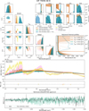 |
Fig. J.12 Same as Fig. J.1 for HIP 79098 (AB) B. |
| In the text | |
Current usage metrics show cumulative count of Article Views (full-text article views including HTML views, PDF and ePub downloads, according to the available data) and Abstracts Views on Vision4Press platform.
Data correspond to usage on the plateform after 2015. The current usage metrics is available 48-96 hours after online publication and is updated daily on week days.
Initial download of the metrics may take a while.