| Issue |
A&A
Volume 708, April 2026
|
|
|---|---|---|
| Article Number | A157 | |
| Number of page(s) | 10 | |
| Section | Extragalactic astronomy | |
| DOI | https://doi.org/10.1051/0004-6361/202557758 | |
| Published online | 03 April 2026 | |
Identifying Compton-thick AGNs in the COSMOS
II. Searching among mid-infrared selected AGNs
1
School of Physics and Astronomy, Anqing Normal University, Anqing 246133, China
2
Institute of Astronomy and Astrophysics, Anqing Normal University, Anqing 246133, China
3
School of Astronomy and Space Science, Nanjing University, Nanjing, Jiangsu 210093, China
4
Key Laboratory of Modern Astronomy and Astrophysics (Nanjing University), Ministry of Education, Nanjing 210093, China
5
College of Physics and Electronic Engineering, Qujing Normal University, Qujing 655011, China
6
School of Physical Science and Technology, Kunming University, Kunming 650214, China
7
School of Science, Langfang Normal University, Langfang 065000, China
★ Corresponding authors: This email address is being protected from spambots. You need JavaScript enabled to view it.
; This email address is being protected from spambots. You need JavaScript enabled to view it.
Received:
20
October
2025
Accepted:
4
March
2026
Abstract
Context. Compton-thick active galactic nuclei (CT-AGNs), defined by a column density of NH ≥ 1.5 × 1024 cm−2, are so heavily absorbed that their X-ray emission is often feeble and can even be undetectable by X-ray instruments in some cases. Nevertheless, their radiation is expected to be a substantial contributor to the cosmic X-ray background (CXB), predicting that CT-AGNs would comprise at least ∼30% of the total AGN population.
Aims. Cosmological Evolution Survey (COSMOS) reported that the identified CT-AGN fraction falls far below theoretical expectations, indicating that a substantial population of CT-AGNs is hidden due to their low photon counts or due to their flux lying below the current flux limits of X-ray instruments. This work focuses on identifying CT-AGNs hidden among mid-infrared (MIR) selected AGNs.
Methods. First, we selected a sample of 1,104 MIR-selected AGNs that were covered, but individually undetected by X-ray. Next, we reduced the X-ray data in the COSMOS and analyzed multiwavelength data in our sample to derive the key physical parameters required for the CT-AGN identification.
Results. Using MIR diagnostics, we found 7 to 23 CT-AGN candidates. Their subsequent X-ray stacking analysis revealed a clear detection at > 3σ significance in the soft band and only a > 1σ significance in the hard band. We fit the stacked soft- and hard-band fluxes with a physical model and confirm that these sources are absorbed by Compton-thick material. However, CT-AGNs ultimately constituted only 2.1% (23/1104) of our sample, significantly below the fraction predicted by CXB synthesis models. This indicates that a considerable population of CT-AGNs remains missed by our selection. A comparison of host-galaxy properties between CT-AGNs and non-CT-AGNs reveals no significant differences.
Key words: galaxies: active / galaxies: nuclei / infrared: galaxies / X-rays: diffuse background
© The Authors 2026
 Open Access article, published by EDP Sciences, under the terms of the Creative Commons Attribution License (https://creativecommons.org/licenses/by/4.0), which permits unrestricted use, distribution, and reproduction in any medium, provided the original work is properly cited.
This article is published in open access under the Subscribe to Open model. This email address is being protected from spambots. You need JavaScript enabled to view it. to support open access publication.
1. Introduction
Active galactic nuclei (AGNs) are defined as galaxies hosting supermassive black holes (SMBHs, 106 − 109 M⊙) that have an Eddington ratio1 exceeding the limit of 10−5 (Netzer 2015). These systems are powered by the accretion of surrounding matter through the SMBHs, thereby releasing their gravitational potential energy. Their emissions cover the entire electromagnetic spectrum, exhibiting distinct radiation characteristics at varying distances from the central SMBHs. The AGN unification model suggests that the radiation across different bands originates from their specific substructures (Antonucci 1993; Urry & Padovani 1995; Netzer 2015). For instance, the accretion disk near the SMBH is heated by the viscous dissipation of gravitational potential energy during mass accretion, producing a broad ultraviolet (UV) to optical continuum spectrum (e.g., Richstone & Schmidt 1980). The hot corona, hovering above the accretion disk, generates luminous X-ray emission through inverse Compton up-scattering of UV–optical photons originating from the accretion disk (Liang 1979; Haardt & Maraschi 1991). The dusty torus, situated outside the corona and accretion disk, absorbs the intense radiation from the central engine and reprocesses it into thermal emission at longer mid-infrared (MIR) band (e.g., Antonucci 1993). Owing to the evolutionary stages of AGNs and the viewing angle effects, the majority of AGNs are obscured by large amounts of dust and gas (e.g., Hickox & Alexander 2018). The high penetration ability of X-ray radiation, combined with the bright X-ray emissions from AGNs, makes X-rays an essential tool for distinguishing AGNs from other extragalactic sources and for investigating the obscured material within AGNs (e.g., Xue 2017). The neutral hydrogen column density (NH) is a key parameter for describing the obscured AGNs in the X-ray band. The obscured AGNs exhibiting a column density of NH ≥ 1.5 × 1024 cm−2 are classified as Compton-thick AGNs (CT-AGNs; e.g., Comastri 2004).
The cosmic X-ray background (CXB) is the radiation from the superposition of all discrete X-ray point sources and AGNs account for the vast majority of these sources (Mushotzky et al. 2000; Moretti et al. 2003; Luo et al. 2017). The most prominent observational feature of the CXB spectrum is a pronounced hump, marking the peak of its energy density, around 30 keV (Revnivtsev et al. 2003; Churazov et al. 2007; Frontera et al. 2007; Ajello et al. 2008). Over the past several decades, theoretical modeling of the CXB spectrum has repeatedly demonstrated that only AGN population synthesis models incorporating a substantial fraction of CT-AGNs can successfully reproduce the complete spectral shape of the CXB (e.g., Gilli et al. 2007; Treister et al. 2009; Burlon et al. 2011; Akylas et al. 2012; Ueda et al. 2014; Ananna et al. 2019; Georgantopoulos et al. 2025). To date, the fraction of CT-AGNs remains uncertain and is a subject of hot debate. At low redshifts, as in the case of the Local Universe, AGN population synthesis models predict that CT-AGNs account for 20–30% of the total AGN population detected by hard X-ray surveys such as Swift-BAT (Burlon et al. 2011; Ueda et al. 2014; Ricci et al. 2015). The denser atomic and molecular gas content in high-redshift galaxies (e.g., Carilli & Walter 2013), relative to the Local Universe, increases the likelihood that AGNs hosted in these environments are heavily obscured, thereby leading to a higher expected fraction of CT-AGNs. For instance, Buchner et al. (2015) estimated that CT-AGNs account for  of the total AGN population in X-ray deep-field surveys, while Ananna et al. (2019) found that this fraction increases to 56%±7% for AGNs throughout redshift z ≃ 1.
To observationally recover the intrinsic fraction of CT-AGNs in the total AGN population, it is essential to select an AGN sample that is unbiased against CT-AGNs. AGN samples selected through MIR methods meet this criterion due to the lower extinction at this waveband (e.g., Li & Draine 2001). Some studies have estimated that the fraction of CT-AGNs in MIR-selected AGN samples aligns with the theoretical predictions for the CXB (e.g., Carroll et al. 2023; Akylas et al. 2024; Lyu et al. 2024). Recently, Annuar et al. (2025) directly measured a CT-AGN fraction of  in a MIR-selected AGN sample within 15 Mpc, where the column densities are derived from broad-band X-ray spectral analysis. Similarly, Boorman et al. (2025) directly measured the CT-AGN fraction of 35%±9% in a sample of 122 nearby (z < 0.044) AGNs primarily selected for their MIR colors. These results have already provided compelling evidence to support the AGN synthesis models of the CXB.
Nevertheless, attaining the theoretically anticipated fraction of CT-AGNs within X-ray surveys remains a significant challenge. The X-ray radiation of CT-AGNs is typically extremely faint, so their photon counts are low and often even undetectable. These characteristics make CT-AGNs the most difficult population to detect in X-ray surveys (e.g., Matt et al. 2000; Comastri et al. 2015; Padovani et al. 2017). In particular, for sources with column densities NH ≥ 1025 cm−2, even in the Local Universe, X-ray flux-limited surveys are biased against detecting CT-AGNs (e.g., Ricci et al. 2015; Koss et al. 2016; Annuar et al. 2025; Boorman et al. 2025). X-ray surveys typically report an observed fraction of CT-AGNs below 15% (e.g., Ricci et al. 2017b; Masini et al. 2018; Georgantopoulos & Akylas 2019), which is significantly lower than theoretical model predictions, meaning that a large number of CT-AGNs remain unidentified or undiscovered. These missing CT-AGNs may still be hidden in AGNs that exhibit low photon counts (e.g., Lambrides et al. 2020) or that have not been detected by X-ray surveys (e.g., Carroll et al. 2021). To identify the missing CT-AGNs in the Local Universe, the X-ray astronomy group at Clemson University and the extragalactic astronomy group at the INAF-OAS Bologna and INAF-IASF Palermo initiated a targeted project in 2017 to actively search for CT-AGNs, known as the Clemson-INAF CT-AGN Project (Marchesi et al. 2018). The project used a volume-limited sample of CT-AGNs with NuSTAR spectra, achieving a CT-AGN fraction of 20%±5% within the redshift of z < 0.01 (Torres-Albà et al. 2021). Similarly, a series of studies have focused on searching for the missing CT-AGNs in X-ray deep-field surveys. For example, Guo et al. (2021) identified eight missing CT-AGNs by using the multiwavelength techniques in the Chandra Deep Field-South (CDFS) survey. Zhang et al. (2025) used machine learning algorithms to identify 67 missing CT-AGNs, thereby raising the fraction of CT-AGNs to 20% in the CDFS survey. Numerous efforts have been made to search for the missing CT-AGNs in X-ray surveys, yet the theoretical expectations remain unmet.
The Cosmic Evolution Survey (COSMOS; e.g., Scoville et al. 2007) is a deep, multiwavelength survey covering a relatively large area of 2 deg2, aimed at measuring the evolution of galaxies and AGNs. The X-ray observations of this field are also crucial for resolving the CXB (e.g., Buchner et al. 2015). The Chandra X-ray telescope has covered the entire COSMOS, achieving a relatively deep average exposure (e.g., Civano et al. 2016; Marchesi et al. 2016). However, the observed fraction of CT-AGNs in the COSMOS is significantly lower than theoretical expectations. For example, Lanzuisi et al. (2018) successfully identified 67 CT-AGNs from a sample of 1855 AGNs with high (> 30) photon counts through X-ray spectral fitting. To find out the hidden CT-AGNs in the COSMOS, it is essential to establish and execute a series of specific tasks. Guo et al. (2025) completed the first task and successfully identified 18 CT-AGNs. In this work, we aim to execute and complete the second task, focusing on identifying CT-AGNs among MIR-selected AGNs. This paper is structured as follows. Section 2 presents the data used to select AGNs via MIR colors and details the construction of our final sample. In Sect. 3 we describe the Chandra observations covering COSMOS and their data reduction. Section 4 presents the multiwavelength photometric data for the sample and the corresponding analysis. Section 5 presents our CT-AGN diagnostics, along with a brief discussion of the missing CT-AGNs in our sample and the properties of CT-AGN host galaxies. A brief summary is presented in Sect. 6. We adopted a concordance flat Λ-cosmology with H0 = 67.4 km s−1 Mpc−1, Ωm = 0.315, and ΩΛ = 0.685 (Planck Collaboration VI 2020). All quoted uncertainties correspond to the 1σ (68%) confidence level unless stated otherwise, while upper limits are given at the 3σ level.
2. The MIR-selected AGN sample
2.1. MIR data collation
To construct a high-quality MIR-selected AGN sample, we systematically collated the MIR data. The primary data source was the COSMOS2020 FARMER catalog (Weaver et al. 2022), which provides Spitzer/IRAC four-band (3.6 μm, 4.5 μm, 5.8 μm, and 8.0 μm) photometric data. To meet the requirements for the sample selection, the following constraints were applied to the MIR photometric data:
-
(1)
Sources with redshifts between 0.1 and 2 were selected;
-
(2)
Sources with IRAC magnitudes over the 3σ detection limit were chosen to ensure data reliability;
-
(3)
The flux-to-error ratio in each band was required to be greater than 5 to ensure a high signal-to-noise ratios.
In the COSMOS2020 FARMER catalog, a total of 56,831 sources satisfy the above constraints. We collected the four band flux densities of Spitzer/IRAC for the steps described in the next section.
2.2. Selection of AGN sample
The unique colors of AGNs in the MIR band, especially between 3–5 μm, make their spectra appear redder than those of normal galaxies. Therefore, many studies use this feature to distinguish AGNs from normal galaxies and identify them (e.g., Lacy et al. 2004, 2007, 2013; Donley et al. 2012; Assef et al. 2013; Chang et al. 2017). For example, the IRAC color-color diagrams most commonly used for AGN selection were defined by Lacy et al. (2004, 2007, 2013) and Donley et al. (2012). In this work, we adopted the AGN selection criterion of Donley et al. (2012), which is more stringent than others and yields a highly pure and reliable AGN sample. Figure 1 presents an IRAC color-color diagram, plotting log(f5.8 μm/f3.6 μm) against log(f8.0 μm/f4.5 μm). The sources within the red dashed lines are AGNs selected using the criteria from Donley et al. (2012), totaling 1,545. Among them 252 are X-ray sources, of which nine have been classified as CT-AGNs by Lanzuisi et al. (2018) and Guo et al. (2025).
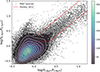 |
Fig. 1. IRAC color–color diagram of the MIR sources. The small gray dots represent all IRAC sources selected in the COSMOS. The region bounded by dashed red lines marks the MIR-AGN selection region of Donley et al. (2012). The sources within this region are classified as MIR-selected AGNs. The color bar and overlaid contours trace the number density gradient across the diagram. |
To identify CT-AGNs among AGNs undetected by X-ray in the COSMOS, we applied the following constraints to the MIR-selected AGN sample:
-
(1)
Remove known X-ray sources from the MIR-selected AGNs;
-
(2)
Eliminate sources lacking X-ray observations (i.e., those with exposure time = 0);
-
(3)
To avoid overestimating the flux upper limits (see Sect. 3.3) of MIR-selected AGNs due to nearby bright X-ray sources, we exclude any sources located within 6″ of known X-ray sources.
After this screening, our final AGN sample comprises 1,104 sources. Columns 1–3 of Table A.1 list their IDs, RA, and DEC. The photometric redshifts of our AGN sample are taken from the COSMOS2020 FARMER catalog, measured by LePhare using the galaxy templates. For the bright sources, Weaver et al. (2022) find a normalized median absolute deviation of only 0.009 in their photometric redshifts; even in the faintest bin (25 mag < i < 27 mag) the normalized median absolute deviation is 0.036. Column 4 of Table A.1 lists their photometric redshifts.
3. X-ray observations and data reduction
3.1. Overview of Chandra’s observations in COSMOS
To identify (or probe) AGNs with varying redshifts in the COSMOS and investigate black hole accretion history, as well as the co-evolution of AGNs with their host galaxies, Elvis et al. (2009) conducted Chandra observations during 2006–2007, accumulating a total exposure of 1.8 Ms. These observations covered the central 0.5 deg2 with an effective exposure of approximately 160 ks and an outer 0.4 deg2 area with an effective exposure of approximately 80 ks. Subsequently, Civano et al. (2016) added further Chandra observations during 2013–2014, increasing the total exposure to 2.8 Ms. These additional observations covered the remaining area (the outer 0.4 deg2 from Elvis et al. 2009) with an effective exposure of approximately 80 ks and increased the effective exposure over the central 1.5 deg2 to approximately 160 ks. As a result, the combined observations totaling approximately 4.6 Ms covered a region of 2.2 deg2 in the COSMOS. For more detailed information on observation files, including observation and exposure times, we refer to Elvis et al. (2009) and Civano et al. (2016).
3.2. Data acquisition and reduction
To determine the X-ray flux upper limits for each AGN in our sample, their exposure times and counts are required. As the exposure and image maps are not archived, we first retrieved all 117 raw event files covering the COSMOS from the Chandra X-ray Center2. Next, we processed these 117 raw event files through the following detailed steps to extract the required exposure times and counts.
We processed the data reduction using CIAO 4.17 software tools (Fruscione et al. 2006) and CALDB 4.12.0. We used the chandra_repro script to reprocess the data, automating the CIAO recommended steps and generating new level 2 event files. Subsequently, we removed ACIS-I Background Flares using the dmcopy and dmextract scripts, following the standard Science Threads from the Chandra X-ray Observatory. Finally, all 117 observations were merged with the merge_obs script to produce exposure-corrected images and the corresponding modeled background maps.
3.3. X-ray luminosity upper limit estimations
Our MIR-selected AGNs are individually undetected in X-rays, their X-ray luminosities cannot be measured directly. Consequently, we quote only upper limits, calculated with the equation (Alexander et al. 2003):

where DL is the luminosity distance,  represents the upper limit of the flux in the 2–10 keV within the observed frame, z is the redshift, and Γ is the photon index used for k-corrections, which is fixed to the value of 1.4 (Civano et al. 2016). The upper limit of the X-ray flux density is calculated by

where Rlim is the upper limit of the count rate at the undetected source and CF is the energy conversion factor, set to 3.06 (Civano et al. 2016). The upper limit of the count rate for undetected sources is calculated by

where Texp represents the effective exposure time at the source location, B3″3σ denotes the 3σ upper limit on the background counts measured within a 3″ radius aperture centered on the source. The 3σ upper limit on the background counts can be calculated using Eq. 9 of Gehrels (1986), giving
![Mathematical equation: $$ \begin{aligned} B_{3^{\prime \prime }}^{3\sigma }\approx (B_{3^{\prime \prime }} +1) \left[1-\frac{1}{9(B_{3^{\prime \prime }} +1)} + \frac{3}{3\sqrt{B_{3^{\prime \prime }} +1}}\right]^3 , \end{aligned} $$](/articles/aa/full_html/2026/04/aa57758-25/aa57758-25-eq7.gif)
where B3″ represents the 0.5–8 keV background counts measured within a 3″-radius aperture centecalibrered on the source, after correction for the energy-encircled fraction. The background counts for AGNs are determined by summing all values from a 3″ radius circle centered at their respective coordinates in the modeled background map. Similarly, the exposure times for the AGNs are determined by reading the values from the exposure map at their respective coordinates. Figure 2 shows the coordinates of MIR-selected AGNs on the exposure map and their corresponding exposure times. Columns 5–6 of Table A.1 give the 3″ aperture background counts B3″ and exposure time Texp for each source.
 |
Fig. 2. Merged Chandra exposure map of the COSMOS, overlaid with the positions of MIR-selected AGNs (black dots) used in this work. The color bar indicates the effective exposure time for the corresponding X-ray coverage. |
Applying the calculation process described above, we derived X-ray luminosity upper limits for the entire MIR-selected AGN sample. Columns 7–8 of Table A.1 list the upper limits of flux density and luminosity in the 2–10 keV band.
4. Analysis of multiwavelength data
4.1. Multiwavelength photometric data
Identifying CT-AGNs among MIR-selected AGNs requires ascertaining the MIR radiation from AGNs. Thus, we need to construct the spectral energy distributions (SEDs) for these sources to decompose the AGN’s contribution to the MIR emission. This process requires multiwavelength photometric data.
The multiwavelength photometric data used in this work span the far-UV (FUV; 1526 Å) to the far-infrared (FIR; 500 μm). Among them, the photometric data covering the wavelength range from the FUV to the MIR (27 bands in total) are sourced from the COSMOS2020 FARMER catalog (Weaver et al. 2022). These bands include the GALEX FUV and NUV band, MegaCam U band, CFHT U band, five Subaru HSC bands (g, r, i, z, and y), 12 Subaru Suprime-Cam medium bands (IB427, IB464, IA484, IB505, IA527, IB574, IA624, IA679, IB709, IA738, IA767, and IB827), four VISTA VIRCAM broad bands (Y, J, H, and Ks), and four Spitzer IRAC bands (ch1, ch2, ch3, and ch4). Moreover, the FIR photometric data are sourced from the COSMOS2015 catalog (Laigle et al. 2016), including MIPS 24 μm, PACS 100 μm, PACS 160 μm, SPIRE 250 μm, SPIRE 350 μm, and SPIRE 500 μm. Where photometric data in a given band are missing, we use the corresponding flux upper limits in the SED analysis.
4.2. Analysis of SEDs
The SED analysis of AGNs is a widely used technique that not only provides detailed information about AGNs but also reveals the properties of their host galaxies (e.g., Guo et al. 2020), such as AGN luminosity, rest-frame 6 μm luminosity for the AGN, stellar mass (M★), and the star formation rate (SFR). To conduct the analysis of AGNs in our sample and obtain the required parameters in this work, we used Code Investigating GALaxy Emission (CIGALE; V2022.1; Boquien et al. 2019), an open Python code containing the template of galaxies and AGNs. Since all the sources in our sample are MIR-selected AGNs, we have used templates that incorporate both the galaxy and AGN characteristics to achieve the most accurate SED fitting. The galaxy templates in CIGALE are generated by integrating four distinct modules, including the star formation history (SFH), the single stellar population (SSP) model (Bruzual & Charlot 2003), the dust attenuation (DA; Calzetti et al. 2000), and the dust emission (DE; Draine & Li 2007; Dale et al. 2014). The AGN component in our analysis is a module developed by Fritz et al. (2006). The modules and parameters used for SED fitting are summarized in Table 1. Additionally, for sources using upper flux limits in certain bands, the lim_flag is set to “noscaling”. Given the vast parameter space, quickly constructing a model on the computer is not feasible. Thus, we adopted an iterative methodology to expedite the acquisition of the best-fitting SEDs. Figure 3 shows the best-fitting SED for an AGN. To assess the reliability of the fitted AGN components, we refit SEDs using only the galaxy templates. A markedly better fit (indicated by a lower χ2) with the combined galaxy+AGN templates than with the galaxy-only templates implies that the fitted AGN components can indeed represent the contribution of the actual AGNs in their SEDs. We used the Bayesian information criterion (BIC) to quantify the significance or confidence of the AGN components (see Appendix C of Guo et al. 2025, for details).
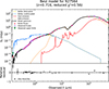 |
Fig. 3. Example of the best-fitting SED for an AGN. The solid black line indicates the best-fitting model. The dashed blue, solid gold, and solid red lines represent unattenuated stellar, attenuated stellar, and dust emission, respectively. The solid apricot line indicates AGN emission. The strawberry filled circles, pastel-purple open circles, and green open inverted triangles denote model predictions, observed fluxes, and observed upper limits, respectively. The lower panel indicates the residual of the best fitting. |
Module assumptions for SED fitting.
Through SED fitting, we obtained the best-fitting SED for each source and derived the corresponding physical parameters. Columns 9–10 of Table A.1 are rest-frame 6 μm luminosity for the AGN and the AGN components’ confidence. Column 11 of Table A.1 presents M★, the derived outcome of SED fitting. However, since the SFR derived from SED fitting relies on the chosen SFH model (Gao et al. 2019), we instead use the calibration method proposed by Bell et al. (2005) to estimate the SFR using UV and IR luminosities. This calibration is scaled to the Chabrier (2003) initial mass function for accuracy. Specifically, the SFR is calculated using the formula,
 (1)
(1)
where LUV = νLν is an estimation of the integrated 1216–3000 Å rest-frame UV luminosity, and LIR is the 8–1000 μm rest-frame IR luminosity. Both LUV and LIR are in units of L⊙. Column 12 of Table A.1 lists the SFR of each source.
5. Diagnostic CT-AGNs and discussion
5.1. MIR diagnostics
The emissions from the corona and dust torus of AGNs are considered good tracers of the accretion disk’s emission. Consequently, a strong correlation is expected between X-ray and MIR emissions in AGNs. Several studies have investigated this relationship in radio-quiet AGNs (e.g., Fiore et al. 2009; Mateos et al. 2015; Stern 2015; Chen et al. 2017; Esparza-Arredondo et al. 2019, 2021). Due to the low optical depth in the MIR band, the MIR radiation from CT-AGNs is not significantly suppressed. As the column density increases, the torus absorbs more nuclear X-ray emission and re-radiates it in the MIR, potentially boosting the MIR luminosity. However, this effect is extremely weak: the AGN X-ray luminosity is 1–2 dex below its UV–optical continuum (Steffen et al. 2006; Lusso et al. 2010), so even complete absorption and re-radiation in the MIR would contribute negligibly compared with the direct disk-dust heating. Ricci et al. (2017b) indeed found no significant increase in MIR luminosity with column density. Consequently, the intrinsic X-ray and MIR luminosities of AGNs are still expected to follow the above relations. However, because the X-ray radiation of CT-AGNs is heavily absorbed, their observed X-ray luminosities fall below the values predicted by these relations. Given that the AGNs in our sample are not detected in X-rays, we adopted the corresponding X-ray luminosity upper limits as their observed luminosities and use these relationships to identify CT-AGNs.
Figure 4 shows the observed X-ray luminosity in the rest-frame 2–10 keV band as a function of the 6 μm luminosity for the fit AGN component. The solid purple, blue, and black lines represent the relation for Chen et al. (2017), Stern (2015), and Fiore et al. (2009), respectively. Assuming the intrinsic 2–10 keV spectrum of each AGN is modeled in in Xspec with phabspowerlaw+constantpowerlaw+pexmon (see Appendix D of Guo et al. 2025 for details), the dashed lines represent the same relationships between MIR and X-ray luminosities after the X-ray spectra have been absorbed by gas with a column density of NH = 1.5 × 1024 cm−2. This means that the sources within or below the shaded area in Fig. 4 should be classified as CT-AGNs. Circles tipped with downward arrows denote the AGNs in our sample, their colors indicating the confidence levels of the fitted AGN components. As shown in Fig. 4, 23 AGNs fall within or below the shaded area, suggesting that they may be CT-AGNs. However, considering the variability in the relations provided by Chen et al. (2017) and Fiore et al. (2009), a range of possible CT-AGN candidates is 7 to 23. To further determine whether they are CT-AGNs, we must assess the reliability of their fitted AGN components. These sources, whose fitted AGN components exhibit a high confidence coefficient (αAGN > 0.95), support a CT-AGN classification; whereas those with a low confidence coefficient (αAGN < 0.95) cannot be reliably identified as CT-AGNs. Finally, a total of 23 AGNs located within or below the shaded region exhibit high confidence coefficients, supporting their diagnosis as CT-AGNs. These CT-AGNs are marked in Fig. 4 by cutting stars within the large circles. Column 13 of Table A.1 also lists their classification, “1” represents CT-AGN identified in this work.
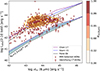 |
Fig. 4. Observed X-ray luminosity in the rest-frame 2–10 keV band as a function of the 6 μm luminosity for fit AGN component. The solid purple, blue, and black lines represent the relation for Chen et al. (2017), Stern (2015), and Fiore et al. (2009), respectively. The dashed lines indicate the same relationships but where the X-ray luminosities are absorbed by a column density of NH = 1.5 × 1024 cm−2. The circles are MIR-selected AGNs with a fit AGN component. The color bar represents the confidence coefficient of the 6 μm luminosity for a fit AGN component (or the fit AGN components). The cutting stars within the large circles represent CT-AGNs identified using the relationship between MIR and X-ray luminosities. |
5.2. Stacking analysis for CT-AGNs
In the preceding section, we successfully find out 7 to 23 CT-AGN candidates. Because these AGNs are individually undetected in X-rays, we cannot extract their X-ray spectra and determine their column densities. To confirm heavy absorption in the X-ray band, we perform X-ray stacking analysis on these 23 AGNs using the publicly available CSTACK V4.5 tool (Miyaji & Griffiths 2008)3. This analysis adopts the default maximum off-axis angle, 3″ source aperture, 6″ background annulus, and automatic exclusion of known X-ray sources. The output of CSTACK includes the stacked photon count rates and their errors for both the soft (0.5–2 keV) and hard (2–8 keV) bands, along with the corresponding stacked images. Figure 5 presents the stacking results: the stacked AGNs are clearly detected at > 3σ significance in the soft band and marginally detected at > 1σ in the hard band. The stacked photon count rates in the soft and hard bands are (1.31 ± 0.39)×10−5 cts s−1 and (7.64 ± 5.06)×10−6 cts s−1, respectively.
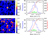 |
Fig. 5. X-ray stacking results for the 23 CT-AGNs identified by MIR diagnostics. Left: Stacked images in the 0.5–2 keV (top) and 2–8 keV (bottom) bands. Right: Corresponding bootstrap histograms of the net count rates. Green lines indicate the mean count rates and 1σ confidence intervals. Detections exceed 3σ significance in the soft band, while only exceeding a 1σ significance in the hard band. |
Assuming the AGN X-ray emission follows a simple power-law spectrum with photon flux density F(E) ∝ E−Γ, we convert the soft- and hard-band count rates into photon fluxes by adopting effective areas of 600 cm2 and 350 cm2, and mean photon energies of 1.2 keV (soft) and 4.0 keV (hard). This derives a photon index Γ = 0.0 ± 0.6. Assuming a Galactic absorption of NH = 2.6 × 1020 cm−2, we use a tool of PIMMS V4.154 to estimate soft- and hard-band fluxes of (7.57 ± 2.25) × 10−17 erg cm−2 s−1 and (2.34 ± 1.55) × 10−16 erg cm−2 s−1, respectively.
To further constrain the absorption of these sources, we fitted the soft- and hard-band fluxes in Xspec with the zphabszpowerlw+constantzpowerlw+pexmon model. The redshift was fixed at the mean value of the 23 sources (z = 0.92), the photon index at 1.9, the inclination angle at 85, and the scattered fraction at 0.005; only the column density, NH, and normalization norm were allowed to vary, while all remaining parameters were kept at their default values. Figure 6 presents the p-value distribution in the log NH–log norm plane obtained by fitting the soft- and hard-band fluxes with our model. In log NH–log norm plane, the data are consistent with the model at the 95% confidence level within two distinct parameter regions, corresponding to Compton-thin and Compton-thick solutions, respectively. The golden solid circles mark the best-fitting points in both regions, with corresponding column densities of 2.09 × 1022 cm−2 and 9.55 × 1025 cm−2, respectively. The X-ray upper limits of these 23 sources already fall below the relationships between MIR and X-ray luminosities after absorbing by Compton-thick material. If their absorption were located in the Compton-thin region, the majority of them would have to be intrinsically X-ray weak AGNs. However, the intrinsic incidence of X-ray weak AGNs is far lower than that of CT-AGNs, making it extremely improbable that most of them are X-ray weak AGNs. The Compton-thin solution can therefore be ruled out. Within Compton-thick region, the 95% confidence level demands log NH > 24.38, while the 90% confidence level requires log NH > 24.76. Both thresholds lie well above the Compton-thick limit, providing direct and compelling evidence that these sources are CT-AGNs. As the hard X-ray band is only marginally detected (slightly above 1σ) in the stacked spectrum, we conservatively treated its flux as an upper limit. Fitting the same model under this assumption still allows us to obtain a solution consistent with Compton-thick absorption.
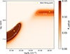 |
Fig. 6. p-value distribution in the log NH–log norm plane. White contours mark p = 0.05, 0.10 and 0.32. The golden solid circle indicates the best-fit point. |
5.3. Missed diagnosis of CT-AGNs
Although MIR-selected AGN samples are incomplete, numerous studies have shown that their CT-AGN fraction closely matches (and even has the potential to reach) the theoretical expectation of CXB (e.g., Lyu et al. 2024; Boorman et al. 2025; Annuar et al. 2025). Our MIR-selected sample excludes X-ray-detected AGNs, which preferentially select less absorbed AGNs. Consequently, we expect the CT-AGN fraction in our MIR-selected sample to markedly exceed that predicted by CXB models. However, our MIR diagnostics identified only 23 CT-AGNs, 2.1% (23/1104) of the MIR-selected sample, significantly below the fraction expected from CXB synthesis models. This discrepancy clearly exceeds statistical error, indicating that MIR diagnostics miss a large number of CT-AGNs. Based on our analysis of the CT-AGN fraction within our sample, we infer that at least 300 CT-AGNs remain unidentified. With the current data and methods, we are still unable to find these missing CT-AGNs. To identify these missed CT-AGNs, the most direct and efficient approach is to conduct significantly deeper X-ray exposures of the COSMOS in the future. On the one hand, deeper exposures will enhance detection sensitivity, revealing AGNs that are currently buried in the background. This might not only confirm their existence, but also enable column density measurements via X-ray spectral fitting, thereby reliably identifying CT-AGNs. On the other hand, for AGNs that remain undetected even after deep exposures, longer integrations will push their X-ray luminosity upper limits to lows, markedly enhancing the discriminatory power of MIR diagnostics.
5.4. The properties of CT-AGN host galaxies
CT-AGNs are widely regarded as an early, heavily obscured phase of AGN evolution (e.g., Guo et al. 2023). Their growth is intimately coupled to the host-galaxy environment, as evidenced by the tight MBH–σ★ relation (e.g., Ferrarese & Merritt 2000) and the role of AGN feedback in regulating star formation (e.g., Bower et al. 2006). Together, this picture supports a coevolutionary relationship between AGNs and their host galaxies (e.g., Kormendy & Ho 2013). CT-AGNs are considered to preferentially host in galaxies with a significant amount of dense gas (Kocevski et al. 2015; Ricci et al. 2017a). Intense AGN radiation compresses their surrounding dense gas, potentially triggering star formation activity within their host galaxies. The host galaxies of CT-AGNs in the Local Universe exhibit a high level of star formation (e.g., Hopkins et al. 2006; Goulding et al. 2012). Zhang et al. (2025) find that the host galaxies of CT-AGNs in the CDFS exhibit higher levels of star formation activity than those of non-CT-AGNs. Andonie et al. (2022) suggested that obscured AGNs have star formation rates that are about three times higher than unobscured systems in the COSMOS. However, Gilli et al. (2022) suggested that the host galaxies of high-redshift AGNs are different from those of AGNs in the Local Universe. Guo et al. (2025) reported similar stellar mass and SFR distributions for CT-AGN and non-CT-AGN host galaxies; while their sample contains only 18 CT-AGNs, which is insufficient for statistically robust conclusions. Using a substantially larger sample, we will re-examine the SFRs and stellar masses of CT-AGN host galaxies relative to those of non-CT-AGNs.
Because a significant number of CT-AGNs in our sample remain unidentified, we were not able to extract a pure non-CT-AGN sample. We therefore adopted the non-CT-AGNs provided by Guo et al. (2025) as the control sample and then combined their CT-AGNs with the 23 newly identified in this work to construct the final CT-AGN sample. Figure 7 presents relationships, represented by the main sequence, between SFRs and stellar masses of the host galaxies for both CT-AGNs and non-CT-AGNs. A Kolmogorov–Smirnov test (KS test) of stellar mass distributions for their host galaxies gave us p = 0.33, while repeating the KS test on their SFR distributions yielded p = 0.20. Although these values are slightly lower than those reported by Guo et al. (2025), they still indicate that there is no significant difference between the two distributions. Thus, our findings do not support any correlation between intense star formation and CT-AGNs, as reported by Zhang et al. (2025). This finding is likely due to the limited size of our CT-AGN sample, which is still too small for statistically robust conclusions. In future works, we will enlarge the CT-AGN sample and further study whether there are differences in the host galaxies of both CT-AGNs and non-CT-AGNs.
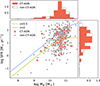 |
Fig. 7. Relationship of the main sequence in AGN host galaxies. The solid red stars indicate the CT-AGNs and the gray circles represent non-CT-AGNs. |
6. Summary
In this work, we aim to identify CT-AGNs hidden in AGNs whose X-ray flux is below the current flux limits in the COSMOS. First, we selected a sample of 1104 MIR-selected AGNs that were covered, but individually undetected in X-ray. Then, we reduced the Chandra observational data covering the field and derived upper limits on the X-ray luminosity for all AGNs in our sample. We subsequently collected multiwavelength photometric data for the sample and extracted key physical parameters for each source through SED fitting, such as six μm luminosities for AGNs, stellar masses, and SFRs. In the next step, using an MIR diagnosis, 7 to 23 sources could be identified as CT-AGNs. To confirm that our CT-AGNs are indeed heavily absorbed in the X-ray band, we performed a stacking analysis. The stacked signal was detected at 3σ significance in the soft band, with a flux of (7.57 ± 2.25) × 10−17 erg cm−2 s−1, whereas the hard-band excess is only 1σ significant, corresponding to (2.34 ± 1.55) × 10−16 erg cm−2 s−1. Fitting the stacked soft- and hard-band fluxes with the zphabszpowerlw+constantzpowerlw+pexmon model allowed us to obtain two parameter regions that are consistent with the data at the 95% confidence level, corresponding to Compton-thin and Compton-thick solutions, respectively. The Compton-thin solution can be ruled out, leaving the Compton-thick absorber as the only viable scenario and confirming these sources as CT-AGNs. We fit their soft- and hard-band fluxes with the zphabszpowerlw+constantzpowerlw+pexmon model and found that when Compton-thick absorption was included, the model did provide a satisfactory fit to both bands. This provides direct and compelling evidence that these sources are CT-AGNs. Although we have already identified some CT-AGNs in the MIR-selected AGNs, a considerable population of CT-AGNs was still missed by our selection. Therefore, we have estimated and discussed the number of missed CT-AGNs in our sample and proposed a practical strategy to search for them. Finally, based on our comparison of host-galaxy properties between CT-AGNs and non-CT-AGNs, we did not find any evidence to support a correlation between intense star formation and CT-AGNs.
Data availability
Table A.1 is available at the CDS via https://cdsarc.cds.unistra.fr/viz-bin/cat/J/A+A/708/A157.
Acknowledgments
We sincerely thank the anonymous referee for useful suggestions. We acknowledge the support of the National Nature Science Foundation of China (No. 12303017). This work is also supported by Anhui Provincial Natural Science Foundation project number 2308085QA33. QSGU is supported by the National Nature Science Foundation of China (Nos. 12192222, 12192220, and 12121003). L.S.Y. is supported by the National Nature Science Foundation of China (No. 12503011). F.L. is is supported by the National Nature Science Foundation of China (No. 12403042). Y.Y.C. is grateful for funding for the training Program for talents in Xingdian, Yunnan Province (2081450001). X.L.Y. acknowledges the grant from the National Nature Science Foundation of China (No. 12303012), Yunnan Fundamental Research Projects (No. 202301AT070242). H.T.W is supported by the Hebei Natural Science Foundation of China (No. A2022408002).
References
- Ajello, M., Greiner, J., Sato, G., et al. 2008, ApJ, 689, 666 [Google Scholar]
- Akylas, A., Georgakakis, A., Georgantopoulos, I., Brightman, M., & Nandra, K. 2012, A&A, 546, A98 [NASA ADS] [CrossRef] [EDP Sciences] [Google Scholar]
- Akylas, A., Georgantopoulos, I., Gandhi, P., Boorman, P., & Greenwell, C. L. 2024, A&A, 692, A250 [NASA ADS] [CrossRef] [EDP Sciences] [Google Scholar]
- Alexander, D. M., Bauer, F. E., Brandt, W. N., et al. 2003, AJ, 125, 383 [Google Scholar]
- Ananna, T. T., Treister, E., Urry, C. M., et al. 2019, ApJ, 871, 240 [Google Scholar]
- Andonie, C., Alexander, D. M., Rosario, D., et al. 2022, MNRAS, 517, 2577 [NASA ADS] [CrossRef] [Google Scholar]
- Annuar, A., Alexander, D. M., Gandhi, P., et al. 2025, MNRAS, 540, 3827 [Google Scholar]
- Antonucci, R. 1993, ARA&A, 31, 473 [Google Scholar]
- Assef, R. J., Stern, D., Kochanek, C. S., et al. 2013, ApJ, 772, 26 [Google Scholar]
- Bell, E. F., Papovich, C., Wolf, C., et al. 2005, ApJ, 625, 23 [Google Scholar]
- Boorman, P. G., Gandhi, P., Buchner, J., et al. 2025, ApJ, 978, 118 [Google Scholar]
- Boquien, M., Burgarella, D., Roehlly, Y., et al. 2019, A&A, 622, A103 [NASA ADS] [CrossRef] [EDP Sciences] [Google Scholar]
- Bower, R. G., Benson, A. J., Malbon, R., et al. 2006, MNRAS, 370, 645 [Google Scholar]
- Bruzual, G., & Charlot, S. 2003, MNRAS, 344, 1000 [NASA ADS] [CrossRef] [Google Scholar]
- Buchner, J., Georgakakis, A., Nandra, K., et al. 2015, ApJ, 802, 89 [Google Scholar]
- Burlon, D., Ajello, M., Greiner, J., et al. 2011, ApJ, 728, 58 [Google Scholar]
- Calzetti, D., Armus, L., Bohlin, R. C., et al. 2000, ApJ, 533, 682 [NASA ADS] [CrossRef] [Google Scholar]
- Carilli, C. L., & Walter, F. 2013, ARA&A, 51, 105 [NASA ADS] [CrossRef] [Google Scholar]
- Carroll, C. M., Hickox, R. C., Masini, A., et al. 2021, ApJ, 908, 185 [NASA ADS] [CrossRef] [Google Scholar]
- Carroll, C. M., Ananna, T. T., Hickox, R. C., et al. 2023, ApJ, 950, 127 [NASA ADS] [CrossRef] [Google Scholar]
- Miyaji, T., Griffiths, R. E., & C-COSMOS Team 2008, AAS/High Energy Astrophys. Div., 10, 4.01 [Google Scholar]
- Chabrier, G. 2003, PASP, 115, 763 [Google Scholar]
- Chang, Y.-Y., Le Floc’h, E., Juneau, S., et al. 2017, ApJS, 233, 19 [Google Scholar]
- Chen, C.-T. J., Hickox, R. C., Goulding, A. D., et al. 2017, ApJ, 837, 145 [Google Scholar]
- Churazov, E., Sunyaev, R., Revnivtsev, M., et al. 2007, A&A, 467, 529 [NASA ADS] [CrossRef] [EDP Sciences] [Google Scholar]
- Civano, F., Marchesi, S., Comastri, A., et al. 2016, ApJ, 819, 62 [Google Scholar]
- Comastri, A. 2004, Compton Thick AGN: the dark side of the X-ray background (Netherlands: Springer), 245 [Google Scholar]
- Comastri, A., Gilli, R., Marconi, A., Risaliti, G., & Salvati, M. 2015, A&A, 574, L10 [NASA ADS] [CrossRef] [EDP Sciences] [Google Scholar]
- Dale, D. A., Helou, G., Magdis, G. E., et al. 2014, ApJ, 784, 83 [Google Scholar]
- Donley, J. L., Koekemoer, A. M., Brusa, M., et al. 2012, ApJ, 748, 142 [Google Scholar]
- Draine, B. T., & Li, A. 2007, ApJ, 657, 810 [CrossRef] [Google Scholar]
- Elvis, M., Civano, F., Vignali, C., et al. 2009, ApJS, 184, 158 [Google Scholar]
- Esparza-Arredondo, D., González-Martín, O., Dultzin, D., et al. 2019, ApJ, 886, 125 [Google Scholar]
- Esparza-Arredondo, D., Gonzalez-Martín, O., Dultzin, D., et al. 2021, A&A, 651, A91 [NASA ADS] [CrossRef] [EDP Sciences] [Google Scholar]
- Ferrarese, L., & Merritt, D. 2000, ApJ, 539, L9 [Google Scholar]
- Fiore, F., Puccetti, S., Brusa, M., et al. 2009, ApJ, 693, 447 [NASA ADS] [CrossRef] [Google Scholar]
- Fritz, J., Franceschini, A., & Hatziminaoglou, E. 2006, MNRAS, 366, 767 [Google Scholar]
- Frontera, F., Orlandini, M., Landi, R., et al. 2007, ApJ, 666, 86 [NASA ADS] [CrossRef] [Google Scholar]
- Fruscione, A., McDowell, J. C., Allen, G. E., et al. 2006, SPIE Conf. Ser., 6270, 62701V [Google Scholar]
- Gao, F.-Y., Li, J.-Y., & Xue, Y.-Q. 2019, Res. Astron. Astrophys., 19, 039 [Google Scholar]
- Gehrels, N. 1986, ApJ, 303, 336 [Google Scholar]
- Georgantopoulos, I., & Akylas, A. 2019, A&A, 621, A28 [NASA ADS] [CrossRef] [EDP Sciences] [Google Scholar]
- Georgantopoulos, I., Pouliasis, E., Ruiz, A., & Akylas, A. 2025, A&A, 695, A128 [NASA ADS] [CrossRef] [EDP Sciences] [Google Scholar]
- Gilli, R., Comastri, A., & Hasinger, G. 2007, A&A, 463, 79 [NASA ADS] [CrossRef] [EDP Sciences] [Google Scholar]
- Gilli, R., Norman, C., Calura, F., et al. 2022, A&A, 666, A17 [NASA ADS] [CrossRef] [EDP Sciences] [Google Scholar]
- Goulding, A. D., Alexander, D. M., Bauer, F. E., et al. 2012, ApJ, 755, 5 [Google Scholar]
- Guo, X., Gu, Q., Ding, N., Contini, E., & Chen, Y. 2020, MNRAS, 492, 1887 [Google Scholar]
- Guo, X., Gu, Q., Ding, N., Yu, X., & Chen, Y. 2021, ApJ, 908, 169 [NASA ADS] [CrossRef] [Google Scholar]
- Guo, X., Gu, Q., Xu, J., et al. 2023, PASP, 135, 014102 [NASA ADS] [CrossRef] [Google Scholar]
- Guo, X., Gu, Q., Fang, G., et al. 2025, A&A, 694, A241 [NASA ADS] [CrossRef] [EDP Sciences] [Google Scholar]
- Haardt, F., & Maraschi, L. 1991, ApJ, 380, L51 [Google Scholar]
- Hickox, R. C., & Alexander, D. M. 2018, ARA&A, 56, 625 [Google Scholar]
- Hopkins, P. F., Hernquist, L., Cox, T. J., et al. 2006, ApJS, 163, 1 [Google Scholar]
- Kocevski, D. D., Brightman, M., Nandra, K., et al. 2015, ApJ, 814, 104 [Google Scholar]
- Kormendy, J., & Ho, L. C. 2013, ARA&A, 51, 511 [Google Scholar]
- Koss, M. J., Assef, R., Baloković, M., et al. 2016, ApJ, 825, 85 [Google Scholar]
- Lacy, M., Storrie-Lombardi, L. J., Sajina, A., et al. 2004, ApJS, 154, 166 [Google Scholar]
- Lacy, M., Petric, A. O., Sajina, A., et al. 2007, AJ, 133, 186 [Google Scholar]
- Lacy, M., Ridgway, S. E., Gates, E. L., et al. 2013, ApJS, 208, 24 [Google Scholar]
- Laigle, C., McCracken, H. J., Ilbert, O., et al. 2016, ApJS, 224, 24 [Google Scholar]
- Lambrides, E. L., Chiaberge, M., Heckman, T., et al. 2020, ApJ, 897, 160 [Google Scholar]
- Lanzuisi, G., Civano, F., Marchesi, S., et al. 2018, MNRAS, 480, 2578 [Google Scholar]
- Li, A., & Draine, B. T. 2001, ApJ, 554, 778 [Google Scholar]
- Liang, E. P. T. 1979, ApJ, 234, 1105 [NASA ADS] [CrossRef] [Google Scholar]
- Luo, B., Brandt, W. N., Xue, Y. Q., et al. 2017, ApJS, 228, 2 [Google Scholar]
- Lusso, E., Comastri, A., Vignali, C., et al. 2010, A&A, 512, A34 [NASA ADS] [CrossRef] [EDP Sciences] [Google Scholar]
- Lyu, J., Alberts, S., Rieke, G. H., et al. 2024, ApJ, 966, 229 [NASA ADS] [CrossRef] [Google Scholar]
- Marchesi, S., Civano, F., Elvis, M., et al. 2016, ApJ, 817, 34 [Google Scholar]
- Marchesi, S., Ajello, M., Marcotulli, L., et al. 2018, ApJ, 854, 49 [Google Scholar]
- Masini, A., Civano, F., Comastri, A., et al. 2018, ApJS, 235, 17 [Google Scholar]
- Mateos, S., Carrera, F. J., Alonso-Herrero, A., et al. 2015, MNRAS, 449, 1422 [Google Scholar]
- Matt, G., Fabian, A. C., Guainazzi, M., et al. 2000, MNRAS, 318, 173 [NASA ADS] [CrossRef] [Google Scholar]
- Moretti, A., Campana, S., Lazzati, D., & Tagliaferri, G. 2003, ApJ, 588, 696 [NASA ADS] [CrossRef] [Google Scholar]
- Mushotzky, R. F., Cowie, L. L., Barger, A. J., & Arnaud, K. A. 2000, Nature, 404, 459 [NASA ADS] [CrossRef] [Google Scholar]
- Netzer, H. 2015, ARA&A, 53, 365 [Google Scholar]
- Padovani, P., Alexander, D. M., Assef, R. J., et al. 2017, A&ARv, 25, 2 [Google Scholar]
- Planck Collaboration VI. 2020, A&A, 641, A6 [NASA ADS] [CrossRef] [EDP Sciences] [Google Scholar]
- Revnivtsev, M., Gilfanov, M., Sunyaev, R., Jahoda, K., & Markwardt, C. 2003, A&A, 411, 329 [NASA ADS] [CrossRef] [EDP Sciences] [Google Scholar]
- Ricci, C., Ueda, Y., Koss, M. J., et al. 2015, ApJ, 815, L13 [Google Scholar]
- Ricci, C., Bauer, F. E., Treister, E., et al. 2017a, MNRAS, 468, 1273 [NASA ADS] [Google Scholar]
- Ricci, C., Trakhtenbrot, B., Koss, M. J., et al. 2017b, ApJS, 233, 17 [Google Scholar]
- Richstone, D. O., & Schmidt, M. 1980, ApJ, 235, 361 [NASA ADS] [CrossRef] [Google Scholar]
- Scoville, N., Aussel, H., Brusa, M., et al. 2007, ApJS, 172, 1 [Google Scholar]
- Steffen, A. T., Strateva, I., Brandt, W. N., et al. 2006, AJ, 131, 2826 [Google Scholar]
- Stern, D. 2015, ApJ, 807, 129 [Google Scholar]
- Torres-Albà, N., Marchesi, S., Zhao, X., et al. 2021, ApJ, 922, 252 [CrossRef] [Google Scholar]
- Treister, E., Urry, C. M., & Virani, S. 2009, ApJ, 696, 110 [NASA ADS] [CrossRef] [Google Scholar]
- Ueda, Y., Akiyama, M., Hasinger, G., Miyaji, T., & Watson, M. G. 2014, ApJ, 786, 104 [Google Scholar]
- Urry, C. M., & Padovani, P. 1995, PASP, 107, 803 [NASA ADS] [CrossRef] [Google Scholar]
- Weaver, J. R., Kauffmann, O. B., Ilbert, O., et al. 2022, ApJS, 258, 11 [NASA ADS] [CrossRef] [Google Scholar]
- Xue, Y. Q. 2017, New Astron. Rev., 79, 59 [Google Scholar]
- Zhang, R., Guo, X., Gu, Q., et al. 2025, ApJ, 987, 46 [Google Scholar]
The Eddington ratio is defined as the ratio of the bolometric luminosity of the AGN to the Eddington luminosity, which represents the balance between the gravitational force and the radiation pressure. For a supermassive black hole with mass MBH, the Eddington luminosity can be approximated as  .
.
CSTACK was developed by Takamitsu Miyaji and is available at https://lambic.astrosen.unam.mx/cstack/
Appendix A: Parameters of MIR-selected AGNs
This section presents a tabular summary of the MIR-selected AGN sample used in this study, the relevant parameters, and the identified CT-AGNs.
Parameters adopted for CT-AGN selection from the MIR-selected AGN sample and summary of the identified CT-AGNs (extract).
All Tables
Parameters adopted for CT-AGN selection from the MIR-selected AGN sample and summary of the identified CT-AGNs (extract).
All Figures
|
Fig. 1. IRAC color–color diagram of the MIR sources. The small gray dots represent all IRAC sources selected in the COSMOS. The region bounded by dashed red lines marks the MIR-AGN selection region of Donley et al. (2012). The sources within this region are classified as MIR-selected AGNs. The color bar and overlaid contours trace the number density gradient across the diagram. |
| In the text | |
|
Fig. 2. Merged Chandra exposure map of the COSMOS, overlaid with the positions of MIR-selected AGNs (black dots) used in this work. The color bar indicates the effective exposure time for the corresponding X-ray coverage. |
| In the text | |
|
Fig. 3. Example of the best-fitting SED for an AGN. The solid black line indicates the best-fitting model. The dashed blue, solid gold, and solid red lines represent unattenuated stellar, attenuated stellar, and dust emission, respectively. The solid apricot line indicates AGN emission. The strawberry filled circles, pastel-purple open circles, and green open inverted triangles denote model predictions, observed fluxes, and observed upper limits, respectively. The lower panel indicates the residual of the best fitting. |
| In the text | |
|
Fig. 4. Observed X-ray luminosity in the rest-frame 2–10 keV band as a function of the 6 μm luminosity for fit AGN component. The solid purple, blue, and black lines represent the relation for Chen et al. (2017), Stern (2015), and Fiore et al. (2009), respectively. The dashed lines indicate the same relationships but where the X-ray luminosities are absorbed by a column density of NH = 1.5 × 1024 cm−2. The circles are MIR-selected AGNs with a fit AGN component. The color bar represents the confidence coefficient of the 6 μm luminosity for a fit AGN component (or the fit AGN components). The cutting stars within the large circles represent CT-AGNs identified using the relationship between MIR and X-ray luminosities. |
| In the text | |
|
Fig. 5. X-ray stacking results for the 23 CT-AGNs identified by MIR diagnostics. Left: Stacked images in the 0.5–2 keV (top) and 2–8 keV (bottom) bands. Right: Corresponding bootstrap histograms of the net count rates. Green lines indicate the mean count rates and 1σ confidence intervals. Detections exceed 3σ significance in the soft band, while only exceeding a 1σ significance in the hard band. |
| In the text | |
|
Fig. 6. p-value distribution in the log NH–log norm plane. White contours mark p = 0.05, 0.10 and 0.32. The golden solid circle indicates the best-fit point. |
| In the text | |
|
Fig. 7. Relationship of the main sequence in AGN host galaxies. The solid red stars indicate the CT-AGNs and the gray circles represent non-CT-AGNs. |
| In the text | |
Current usage metrics show cumulative count of Article Views (full-text article views including HTML views, PDF and ePub downloads, according to the available data) and Abstracts Views on Vision4Press platform.
Data correspond to usage on the plateform after 2015. The current usage metrics is available 48-96 hours after online publication and is updated daily on week days.
Initial download of the metrics may take a while.