| Issue |
A&A
Volume 708, April 2026
|
|
|---|---|---|
| Article Number | A67 | |
| Number of page(s) | 13 | |
| Section | The Sun and the Heliosphere | |
| DOI | https://doi.org/10.1051/0004-6361/202557951 | |
| Published online | 26 March 2026 | |
Electron Acceleration Simulations (EASI): An open-source tool to simulate electron acceleration in shocks
1
Department of Physics and Astronomy, University of Turku, Turku, Finland
2
Department of Physics and Astronomy, Queen Mary University of London, London, United Kingdom
3
Centre for Mathematical Plasma Astrophysics, KU Leuven, Leuven, Belgium
★ Corresponding author: This email address is being protected from spambots. You need JavaScript enabled to view it.
Received:
3
November
2025
Accepted:
23
February
2026
Abstract
Aims. The aim of the this work is to investigate electron acceleration in shocks and present an easy-to-use simulation model that can be used to check resulting energetic particle populations from shock interactions.
Methods. A new open-source model is presented in the work for investigation of electron acceleration and electron beam generation and for further research within the heliophysics community. The model is a one-dimensional Monte Carlo model with physical input parameters, in which particles obey a transport equation in a large-scale field with focusing caused by magnetic field gradients and in which the effects of a small-scale turbulent field on charged particles are described by pitch-angle scattering. The shock has a finite thickness and an adjustable mean free path profile. Particles are injected monoenergetically and with energies sampled from a Maxwellian distribution to investigate attained energies and beam generation.
Results. The simulation results indicate that particles can be accelerated to energies of >100 keV from a 1 keV monoenergetic injection with plasma and shock parameters corresponding to coronal shock environments. An electron beam linked to radio observations of shock waves can also be generated with sufficiently high shock obliquities and, in particular, with a Maxwellian distribution of particle injection energies. Moreover, as the model performs computationally well and corresponds to expectations based on physics, it is an excellent tool for investigating energetic electrons and radio observations corresponding to the electron beams generated in shock waves.
Key words: magnetohydrodynamics (MHD) / shock waves / turbulence / Sun: corona / Sun: coronal mass ejections (CMEs) / Sun: particle emission
© The Authors 2026
 Open Access article, published by EDP Sciences, under the terms of the Creative Commons Attribution License (https://creativecommons.org/licenses/by/4.0), which permits unrestricted use, distribution, and reproduction in any medium, provided the original work is properly cited.
This article is published in open access under the Subscribe to Open model. This email address is being protected from spambots. You need JavaScript enabled to view it. to support open access publication.
1. Introduction
The highly energetic processes of solar eruptions not only influence the near-Earth space environment but also provide critical insights into particle acceleration mechanisms in astrophysical plasmas. Diffusive shock acceleration (DSA; Axford et al. 1977; Krymskii 1977; Bell 1978; Blandford & Ostriker 1978) has been shown to be able to account for high-energy particle acceleration in shock waves of solar coronal mass ejections (CMEs; see, e.g., Nyberg et al. 2024, and references therein), and accounts for proton acceleration from thermal to high energies, but remains inefficient in terms of electron acceleration. Nonrelativistic electrons do not participate in DSA efficiently, as their mean free paths are large (see, e.g., Dröge 2005) and, because of their low mass, their speeds are high, leading to large DSA timescales. In coronal and heliospheric shocks DSA timescales of nonrelativistic electrons become large compared to the lifetime of the shock and in the context of astrophysical shocks, the electron injection problem remains (see, e.g., Riquelme & Spitkovsky 2011) as thermal electrons simply do not participate efficiently enough to DSA.
Coronal shocks are typically driven by CMEs, propagating through the solar corona and into the interplanetary medium. As these shocks traverse the tenuous and magnetized plasma of the corona, they can efficiently accelerate charged particles, including electrons, to relativistic speeds. Observations have provided compelling evidence of electron acceleration associated with coronal shock waves (see, e.g., Mann & Klassen 2005; Carley et al. 2013; Morosan et al. 2022; Dresing et al. 2022). Electron acceleration in shocks has also been recently studied by Xu et al. (2025). Additionally, radio observations of shocks depend on anisotropic high-energy electrons generating Langmuir waves (see, e.g., Mann et al. 2018). Alongside the investigation of the attained energies, the electron beam generation needs to be investigated when considering the performance of models regarding particle acceleration in coronal shock waves.
Discussing electron acceleration models in particular, shock drift acceleration (SDA) has been investigated as a potential mechanism for electron injection to the DSA regime, but results have pointed toward SDA not being sufficient in accelerating particles (see, e.g., Vandas 2001). Thermal electrons are too low in energy to be reflected from the shock or pass from the downstream to the upstream, leading to the need for a model that explains low-energy electron energization in shocks. A modification of SDA, stochastic shock drift acceleration (SSDA; Katou & Amano 2019; Amano & Hoshino 2022; Amano 2022; Lindberg et al. 2023; Amano et al. 2024), has garnered attention as a promising model to explain the injection of suprathermal electrons into shock waves.
The SDA mechanism involves the interaction of charged particles with a shock wave in the presence of a magnetic field. SDA is efficient in quasi-perpendicular shocks, where particles experience a magnetic gradient drift along the shock front and are accelerated by the upstream convection electric field. In the context of the solar corona, where the magnetic field is highly structured and the plasma conditions vary significantly, the plasma conditions might be good for SDA in some regions. To extend these regions and give way to more particle acceleration, we extend the classical SDA model to include stochastic effects, giving rise to the SSDA model. This model accounts for the strongly fluctuating small-scale fields in the shock ramp, where particles may undergo strong scattering, leading to a stochastic increase in energy. Differing from DSA, in SSDA the particles are trapped by the turbulence in the shock transition layer and are accelerated by the convection electric field. Thus, unlike DSA, SSDA does not depend on the level of turbulence in the ambient medium.
In this study, we present a detailed investigation of electron acceleration in coronal shock waves with different acceleration regimes in place. We have developed a comprehensive model that incorporates the key physical parameters of the coronal shock environment, such as the magnetic field geometry, shock speed, and plasma density. By simulating the interaction of electrons with coronal shocks, we aim to investigate the efficiency of DSA, SDA, and SSDA in producing the high-energy electron populations observed in solar events and producing a beamed electron population to further elucidate the radio observations of shocks known to be caused by accelerated electrons.
2. Model
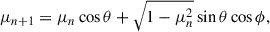
The simulation model presented in this paper is open-source1 and modular, allowing for implementation and investigation of different kinds of plasma environments and can be used as a basis for more complex scenarios in future studies. The model is one-dimensional (1D) in space and based on the Monte Carlo methodology, whereby particles are traced under guiding-center approximation in a large scale field with focusing and whereby the effect of a small-scale turbulent field on charged particles is described by stochastic pitch-angle scattering (e.g., Vainio et al. 2000). The model describes particles accelerated in a shock with a finite width (Fig. 1) and a variable turbulent environment controlled by the parametrization of the mean free path of the particles.
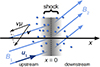 |
Fig. 1. Depiction of the 1D simulation model geometry in HTF. The singular spatial dimension of the model is along the shock normal, denoted as x. A finite-thickness shock is set at x = 0, with the upstream and downstream of the shock modeled with free-escape boundaries far from the shock. Particles travel along the magnetic field lines and particles’ position is tracked along x. Particle speed, v, pitch-angle cosine, μ, and residence time, t − t0, within the simulation box are also tracked. |
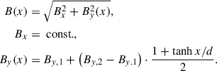
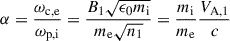
The spatial dimension of the simulation is along the shock normal line, x. The shock has a finite thickness on the order of an ion inertial length, di, which is apparent in the magnetic field profile,
 (1)
(1)
where subscripts 1 and 2 indicate upstream and downstream values, respectively, x is the position in the shock normal direction, Bx is the magnetic field component along the shock normal vector, By is the magnetic field component perpendicular to the shock normal vector, and d(=di) is the shock ramp width. An ion inertial length was chosen as the shock ramp width for simplification of the parametrization. Though the literature suggests a value on the order of the ion gyroradius solved using the upstream flow speed rc = ux, 1/ωc, i (e.g., Livesey et al. 1984, and references therein), the choice of the ion inertial length (di = vA/ωc, i) only differs by a factor of the inverse of the Alfvén Mach number, and as models, such as the one used by Amano & Hoshino (2022), use a scaling factor on the order of unity for the ion gyroradius for the shock thickness, this discrepancy is negligible. The resulting obliquity profile is shown in the first panel of Fig. 2, which is of the form
 (2)
(2)
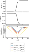 |
Fig. 2. Zoom-in on the shock transition region of the simulation showcasing the local magnetic field obliquity, the local plasma flow speed in HTF, and the mean free path profile dependent on the gradient of the magnetic field with the input parameters of the simulation listed in Table 1. |
where θBn, 1 is the upstream shock normal angle and rB is the magnetic compression ratio of the shock. The solar wind flow profile was chosen to match the profile of the magnetic field, so that in the global de Hoffmann–Teller frame (HTF) the magnetic field, B, and the plasma flow velocity, u, are aligned also in the transition region, and the convection electric field, E = −u × B = 0:
 (3)
(3)
where ux is the flow velocity component along the shock normal vector, uy is the flow velocity component perpendicular to the shock normal vector, and rg is the gas compression ratio of the shock. The flow speed profile is shown in the second panel of Fig. 2.
Electric currents cause numerous microinstabilities in plasma (see, e.g., Muschietti & Lembège 2006; Matsukiyo & Scholer 2006; Lemoine et al. 2014), which can scatter electrons. Hence, as an ad hoc model motivated by such instabilities, the scattering mean free path of the particles was assumed to be proportional to the particle Larmor radius and inversely proportional to the current density (Fig. 2, third panel). A maximum mean free path was set to the simulation as an input parameter. The mean free path in the ambient plasma is independent of particle energy and, through the transition region of the shock, of the form
![Mathematical equation: $$ \begin{aligned} \lambda _{\rm trans} = \frac{\lambda _{\rm 1}}{2} \left[ \left( 1 - C_{\rm ds}\right)\tanh \left(-x/d\right) + 1 + C_{\rm ds} \right], \end{aligned} $$](/articles/aa/full_html/2026/04/aa57951-25/aa57951-25-eq4.gif) (4)
(4)
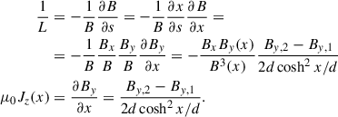
where λ1 is the (global) ambient mean free path in the upstream and Cds the downstream mean free path scaler in relation to the upstream value. The microinstabilities were taken into account as a separate scattering rate (v/λshock) that was linearly superposed with the scattering rate tied to λtrans:
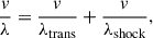 (5)
(5)
giving us the mean free path
 (6)
(6)
where
 (7)
(7)
Here, A is a (dimensionless) normalization factor to tune the minimum allowed mean free path at the shock for a specified energy (for the monoenergetic injection cases in this investigation the chosen energy is the injection energy of 1 keV), c is the speed of light, α = mi/me ⋅ VA, 1/c, v the particle speed in the plasma rest frame, γ the particle’s Lorentz factor, and θBn(x) the local magnetic field obliquity according to Eq. (2). The minimum mean free path case presented in Fig. 2 corresponds to the limit of the mean free path being less than the thickness of the transition region of the shock wave, i.e., the ion inertial length, di.
Physical input parameters of the simulation run presented.
The model has a finite simulation box size, with free escape boundaries in both the upstream and downstream. By default, the simulation box size is determined by the diffusion length of the particles along the magnetic field line calculated at injection energy
 (8)
(8)
where vinj is the injection speed of the particles in the plasma rest frame. A free escape boundary in the upstream acts as a proxy to global focusing, allowing particles to escape the shock vicinity, and has been investigated in depth by Annie John et al. (2024). The free escape downstream can also be used as a proxy due to the particles’ eventual advection out of the box into the downstream.
Particles are injected from the upstream boundary of the simulation box in the plasma rest frame, mono-energetically in the first part of the results (Section 3.1) and with a speed sampled from a Maxwellian distribution in the second part of the results (Section 3.2). The Maxwellian injection was done by sampling the particle injection speeds from the flux-weighted particle distribution
 (9)
(9)
where CM is a normalization factor, v∥ the parallel component of the particle velocity, u1 the local upstream plasma speed in the shock frame, v⊥ the perpendicular component of the particle velocity, kB the Boltzmann constant, T the upstream plasma temperature, me the electron mass, v the particle speed in the plasma rest frame, and vmax the maximum speed sampled from the distribution, after which the pitch-angle cosine was solved from Eq. (A.16).
Particle distribution obeys the focused transport equation (for comprehensive equations see, e.g., Wijsen 2020), incorporating small-angle scattering off of magnetic field fluctuations (here assumed to be elastic in the local-rest frame of the plasma) and focusing in the transition region of the shock due to the magnetic field gradient present. The simulation input parameters were chosen to correspond to typical coronal conditions and are listed in Table 1. The plasma beta in the simulations was solved by using the ambient temperature and Alfvén speed:
 (10)
(10)
The chosen parameters are not intended to be used for experimental validation of the model, but rather as a choice of reasonable input. A detailed description of the simulation implementation is described in Appendix A.
3. Results
The simulation ran until all injected particles escape the simulation box. Particle position x, speed v in HTF, pitch-angle cosine μ in HTF, and other additional variables such as the residence time, t − t0, were saved and used to analyze the results of the simulations. Additionally, time-integrated phase space histograms (see Fig. 5 and text below) were saved and used to analyze the system’s steady state in phase space (see Appendix B for details). Results are plotted in either the plasma rest frame or HTF. The frame is reported in each context where it is relevant.
3.1. Acceleration regimes
The model was run in different mean free path regimes to investigate the plausibility of DSA, SDA, and SSDA as potential acceleration and beam generation mechanisms for electrons. DSA and SSDA were simulated in large simulation boxes, with box size corresponding the injected particles’ diffusion lengths in the plasma rest frame, Lbox = λ1vinjcos2θBn, 1/(3ux, 1), in the shock-normal direction with DSA corresponding to using the ambient plasma and transition mean free path λtrans and SSDA with the four different models of adjusted mean free paths at the shock shown in Fig. 2. Figure 3 contains the energy spectra of the particles in the plasma rest frame for electrons that have escaped either upstream or downstream of the shock. The spectra show acceleration from the injected 1 keV to hundreds of kilo-electronvolts for λamb (black curve) and the factors 10−4 (blue curve) and 10−5 (red curve). The smaller mean free paths at the shock (orange and yellow curves) result in very little acceleration and no particles escaping upstream of the shock. A flat spectrum can be seen in the downstream of the three longer mean free path cases (black, blue, and red curves), in the range of 2–10 keV.
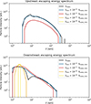 |
Fig. 3. Particle energy spectrum in the plasma rest frame for escaping particle populations upstream and downstream of the shock for different minimum mean free paths at the shock. The box size used in the simulations corresponds to the injected particles’ diffusion length, Lbox ( = λ1vinjcos2θBn, 1/(3ux, 1) ≈ 3.5 ⋅ 105di), upstream and downstream of the shock along the magnetic field line. |
Figure 4 presents the results for a smaller simulation box (20 di to the upstream and downstream) with different minimum mean free paths at the shock. The smaller box size eliminates DSA, as particles are not scattered back to the shock after they have interacted with it, leaving only SDA and, with small mean free paths at the shock, SSDA to be simulated. Only the minimum mean free path factors of 10−4 and 10−5 result in acceleration to tens of kilo-electronvolts in both upstream and downstream, with λamb leading to energies of 10 keV in the upstream. Again, the smaller mean free path factors result in no particles escaping upstream, and very little acceleration in the downstream population.
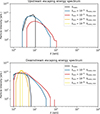 |
Fig. 4. Particle energy spectrum in the plasma rest frame for escaping particle populations upstream and downstream of the shock for different minimum mean free paths at the shock. The box size used in the simulations is 20 di upstream and downstream of the shock along the magnetic field line. |
An efficient way to solve the steady-state particle population inside the box as a function of position and momentum is to gather a histogram of particle data by integrating the particle path over time, i.e., updating the histogram at each time step using the varying time step size of the particle as the weight of each count (Fig. 5, Appendix B). This allows one to compute smooth steady-state solutions of the model using much fewer Monte Carlo particles than when using snapshots.
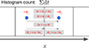 |
Fig. 5. Depiction of the time-integrated phase space histogram of the simulation. As a particle spends a time step, dt, traveling between spatial histogram bins, the time spent in each bin, dt1 and dt2, is added to each respective bin. dt is set to be small enough for particles to not skip spatial bins when propagating through x. |
Figure 6 shows the histogram data over position x, integrated over the whole energy range attained by particles. In the two shorter mean free path cases, the distribution of particles upstream and downstream of the shock are consistent with the gas compression ratio (rg ≈ 3.5) of the shock in the larger and smaller simulation boxes, indicating that particles are mainly advected across the shock as a fluid. There is a peak at the shock for the larger-mean-free-path cases (black and blue curves) with a width of ∼3 di for the larger and smaller simulation box, as particles are interacting with the shock compression. This results from the anisotropies of electrons at the shock transition. A small foot can also be seen in front of the shock. For the larger box size, the ratio of particle densities in the upstream and downstream region is close to unity for the larger mean free paths, consistent with DSA.
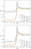 |
Fig. 6. Time-integrated histogram as explained in Fig. 5 of particle positions zoomed in to the vicinity of the shock for the simulation box extending to the injected particles’ diffusion length upstream and downstream (top) and the simulation box extending to 20 di upstream and downstream (bottom) for different minimum mean free paths at the shock. |
The data collection of the histogram can be done multi-dimensionally. Our simulation model collects the particles in a three-dimensional (3D) histogram with the axes of position x, momentum p, and pitch-angle cosine μ. Figure 7 shows the momentum-integrated histogram of pitch-angle cosine μ as a function of position x in HTF for the different mean-free-path cases excluding the factor of 10−8 for the larger simulation box and Fig. 8 for the smaller simulation box. As the shock is nearly perpendicular (θBn = 87°, Table 1), HTF scans the magnetic field line very fast, causing the semi-isotropic particle population in the plasma rest frame at the edge of the simulation box to be quite collimated toward the shock in the HTF (the top left corner of each panel roughly corresponds to the injected population). In the two longest-mean-free-path cases the pitch-angle cosine mainly changes due to the conservation of the adiabatic invariant at the shock, though some scattering also occurs already in the upstream before the particles reach the shock. A collimated electron population propagating away from the shock toward the upstream can be seen in the two shorter-mean-free-path cases in the larger and smaller box, with a very diffuse population of particles propagating away from the shock in the case with the factor of 10−5. As the mean free path decreases, the upstream population propagating away from the shock becomes more diffuse. No particles escape from the downstream back to the upstream in the shortest-mean-free-path case (bottom right panels in Figs. 7 and 8).
 |
Fig. 7. Time-integrated phase space histogram of particles over particle position x and pitch-angle cosine μ in HTF for the simulation box extending to the injected particles’ diffusion length upstream and downstream for the λtrans mean free path profile (first from left), minimum mean free path factor of 10−4 (second from left), minimum mean free path factor of 10−5 (third from left), and minimum mean free path factor of 10−6 (fourth from left). |
 |
Fig. 8. Time-integrated phase space histogram of particles over particle position x and pitch-angle cosine μ in HTF for the simulation box extending to 20 di upstream and downstream for the λtrans mean free path profile (first from left), minimum mean free path factor of 10−4 (second from left), minimum mean free path factor of 10−5 (third from left), and minimum mean free path factor of 10−6 (fourth from left). |
3.2. Beam generation
The electron beam generation was investigated using a Maxwellian injection, whereby particle injection speeds were sampled from a Maxwellian distribution at a temperature of 2 MK in the plasma rest frame to correspond with other coronal parameters of the shock. The mean free path profile, λtrans, was first used with a large box size to keep the shock model simple. The modified mean free path at the shock was investigated later. Different shock obliquities were investigated to see when beam generation takes place. Some of the results of this section are displayed in Appendix C.
To first observe the results of the chosen injection and other parameters, the energy spectra of shock obliquities 70°, 80°, 85°, 86°, 87°, and 88° were investigated. The upstream escaping particle energy spectra in the plasma rest frame are shown in Fig. 9. The lower-obliquity cases, namely the 70° and 80° cases, show particle acceleration extending up to tens of kilo-electronvolts. With increasing obliquity the amount of particles escaping upstream decreases, but the attained cutoff energies increase to hundreds of kilo-electronvolts. Figure 10 shows the energy spectra of particles escaping downstream. The attained energies on the downstream side are otherwise similar, but the highest-obliquity case shows a significant difference in cutoff energy compared to its upstream counterpart.
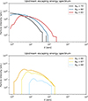 |
Fig. 9. Particle energy spectrum in the plasma rest frame for escaping particle populations upstream of the shock for shock obliquities 70°, 80°, and 85° (top) and 86°, 87°, and 88° (bottom). The box size used in the simulations corresponds to a 1 keV particle’s diffusion length upstream and downstream of the shock along the magnetic field line. The mean free path profile, λtrans, was used. |
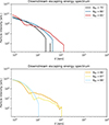 |
Fig. 10. Particle energy spectrum in the plasma rest frame for escaping particle populations downstream of the shock for shock obliquities 70°, 80°, and 85° (top) and 86°, 87°, and 88° (bottom). The box size used in the simulations corresponds to a 1 keV particle’s diffusion length upstream and downstream of the shock along the magnetic field line. The mean free path profile, λtrans, was used. |
Figures C.1 and C.2 show histograms that tracked particle momentum parallel to the magnetic field traveling in the direction from the downstream toward the upstream in the plasma rest frame (antiparallel direction). Additionally, slices along three lines in the antiparallel component are shown denoted by colored arrows and lines. A distinguishable, though faint, electron beam is seen in the cases for 70° and 80° (Fig. C.1), but for the cases of 85°, 86°, 87°, and 88° the electron beam energy range is pushed to the tail end of the spectra, parted from the core of the injected population, allowing it to rise significantly above the spectrum, with the beam density decreasing and beam energy range increasing with increasing obliquity.
Finally, the 86°, 87°, and 88° cases are repeated but with the mean free path profile corresponding to the profile with the scaling factor of 10−4 in Fig. 2. The results in Fig. C.3 look to be otherwise similar to the cases with the λtrans mean free path, though the beam does not seem to form right at shock midpoint (x = 0), but rather only in the upstream, and the beam densities are smaller compared to the λtrans mean free path cases.
4. Discussion
The simulation model results in electrons being accelerated from suprathermal energies (≈1 keV) to hundreds of kilo-electronvolts in coronal environments when using the simulation box extending to the diffusion length of the injected particle’s upstream and downstream of the shock and even with smaller simulation boxes when using small mean free paths (red and blue curves in Fig. 2) at the shock transition region. SDA otherwise accelerates particles very little, though it generates an electron beam relevant for radio bursts observed in correspondence with coronal shock waves also with the λtrans mean free path profile (black curve in Fig. 2) in addition to the reduced mean free path cases. Additionally, the Maxwellian injection results (Figs. 9, C.1, and C.2) would indicate that an electron beam is generated only when electrons with an energy of hundreds of kilo-electronvolts are generated for the chosen shock parameters, though this limit seems soft and parameter-dependent.
Among other radio burst generation parameters, Holman & Pesses (1983) investigated shock obliquity in the context of SDA. As the results of our investigation seem to indicate that the SDA mechanism has a key role in beam generation in all of the cases, the obliquity of the investigation (Holman & Pesses 1983) is important to validate. To generate a beam, the speed of the reflected particles needs to be higher than the speeds of the thermal population, since the thermal population will not participate in the reflection process but simply pass through the shock. For particles to be reflected from the shock their (shock-frame) pitch angles, α, need to be outside the loss cone (sin α > sin α1, c), which is possible only for particles fulfilling the condition
 (11)
(11)
Here, vi is the (plasma-frame) speed of the particle before interacting with the shock, u1 = ux, 1secθBn, and the critical (shock-frame) loss cone pitch-angle sine in the upstream is defined as
 (12)
(12)
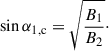
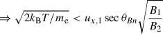
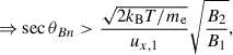
Although the magnetic compression ratio is dependent on the shock obliquity, it is used as a free parameter with the value of B2/B1 = 3.4 (solved from the gas compression ratio, Alfvén Mach number, and shock obliquity of the simulation) as it does not significantly alter the results of the analysis. For the Maxwellian injection, the most likely absolute value of the speed in a 3D Maxwellian distribution,  , where kB is the Boltzmann constant, is used to describe the thermal population. Requiring the initial speed, vi, to be higher than the thermal speed, vth, and solving for the critical obliquity at which particles will be reflected,
 (13)
(13)
 (14)
(14)
 (15)
(15)
results in a minimum value of 84.4° for the obliquity for beam generation, corresponding to the shown results when considering the slice at the shock (red curve) in Fig. C.1 having a beam only in the cases from 85° onward and the slice in the upstream (blue curve) being parted from the thermal injection population. Holman & Pesses (1983) set the upper limit for the obliquity in terms of the beam generation as the angle where one cannot change to HTF, i.e., where the HTF speed exceeds the speed of light, which in our case results in an angle of 89.7°.
The reflection condition can also be interpreted so that it gives the minimum value for upstream particle speed for a set shock obliquity that would generate a beam. Using the reflected speed one can then estimate the theoretical energy of the peak intensity of the beam. The critical velocity for reflection in the upstream plasma rest frame is vi sin α1, c and then the speed in the shock normal direction after reflection is 2u1 − vi sin α1, c which can be simplified to ux, 1secθBn ⋅ (2 − B1/B2). Solving the final speed, and thus the beam peak energy, for the obliquities 70°, 80°, 85°, 86°, 87°, and 88° results in peak energies of 0.139 keV, 0.539 keV, 2.148 keV, 3.365 keV, 6.025 keV, and 13.857 keV, respectively. Comparing to Figs. C.1 and C.2 we can see that the beam peak of the beam in the upstream (blue slice) corresponds well to the numbers, except for the 88° case, in which the theoretical value is roughly 30% larger than what the model produces. This could be caused by the injection population of particles modifying the spectrum, and thus the interpretation made of the beam peak energy, though more investigation is needed to establish a proper interpretation of the discrepancy. This investigation is out of the scope of this paper and will be addressed in future studies. The beam peak energies at the shock (red slice) are always lower than the values in the upstream and predicted theoretically. Therefore, we conclude that the beam energy estimation corresponds well with the obtained results.
The spatial distributions seem to contain a structure that could be interpreted observationally as a shock spike, but this is not the case as the roughly 3 di wide spike in the spatial distribution would correspond to less than a second in the spacecraft frame, a timescale that is only approached by Solar Orbiter’s (Müller et al. 2020) Energetic Particle Detector (EPD; Rodríguez-Pacheco et al. 2020) with its 1 s cadence. The lack of wave generation by wave-particle interactions, of perpendicular diffusion, and of the convection electric field and other electric fields in the model could affect the conclusions that can be drawn from the model.
5. Conclusions and outlook
The attained results of energies of >100 keV from a monoenergetic injection of 1 keV electrons and the formation of an electron beam in particle energies corresponding to theory explaining radio observations of coronal shocks are promising in understanding how relativistic electrons are being injected to DSA in coronal shocks and how the electron populations needed to generate the Langmuir waves for radio observations originate. To really dive into the radio observations, one should investigate the Langmuir wave generation by the beamed electron population self-consistently, and furthermore investigate the effects that the newly generated wave population has on electron acceleration. Similarly, the lack of electric fields in the model could affect the formed structures and attained energies. Regardless, this ad hoc model is enough to investigate roughly particle populations resulting from shock and plasma input parameters, and as such, waves and electric fields are beyond the scope of the present paper, but will be a subject of future development efforts of the model.
With perpendicular shocks, perpendicular diffusion becomes a topic of discussion as well. The more perpendicular a shock is, the more perpendicular diffusion will affect particle transport, and could substantially change the attained energies and beam formation in these results. Including perpendicular diffusion is another path for future development.
The modular model allows the user to test different kinds of parameters for different plasma environments and shock waves, to try different kinds of shock profiles to test how the interpretation of a shock front affects the results, and to implement more physical mechanisms, such as wave-particle interactions and a global magnetic field and its constituents, to see what kind of processes would contribute significantly to reaching a complete understanding of electron acceleration in heliospheric shocks.
The model as it is can be used to understand observations and make predictions and comparisons between spacecraft to paint a more global picture of electron acceleration in the heliosphere. The open-source model allows for further development and implementation of additional physical mechanisms and considerations to investigate all relevant phenomena related to particle acceleration and its signatures in heliospheric plasma environments by any interested reader. The model also works as an excellent educational tool as the modular nature makes it extremely readable and adjustable.
Acknowledgments
This research has received funding from the European Union’s Horizon Europe research and innovation programme under grant agreement No 101134999 (SOLER). The study reflects only the authors’ view and the European Commission is not responsible for any use that may be made of the information it contains. This research has received funding from the Finnish Cultural Foundation, Varsinais-Suomi Regional fund. The computer resources of the Finnish IT Center for Science (CSC) and the FGCI project (Finland) are acknowledged. LV acknowledges the financial support of the University of Turku Graduate School and STFC grant ST/X000974/1. We acknowledge the Research Council of Finland project ‘SolShocks’ (grant number 354409). The work in the University of Turku is performed under the umbrella of Finnish Centre of Excellence in Research of Sustainable Space (FORESAIL; grant no. 352847).
References
- Amano, T. 2022, EGU General Assembly Conference Abstracts, EGU22–3277 [Google Scholar]
- Amano, T., & Hoshino, M. 2022, ApJ, 927, 132 [NASA ADS] [CrossRef] [Google Scholar]
- Amano, T., Masuda, M., Oka, M., et al. 2024, Phys. Plasmas, 31, 042903 [Google Scholar]
- Annie John, L., Nyberg, S., Vuorinen, L., et al. 2024, J. Space Weather Space Clim., 14, 15 [NASA ADS] [CrossRef] [EDP Sciences] [Google Scholar]
- Axford, W. I., Leer, E., & Skadron, G. 1977, Int. Cosm. Ray Conf., 11, 132 [Google Scholar]
- Bell, A. R. 1978, MNRAS, 182, 147 [Google Scholar]
- Blandford, R. D., & Ostriker, J. P. 1978, ApJ, 221, L29 [Google Scholar]
- Carley, E. P., Long, D. M., Byrne, J. P., et al. 2013, Nat. Phys., 9, 811 [Google Scholar]
- Dresing, N., Kouloumvakos, A., Vainio, R., & Rouillard, A. 2022, ApJ, 925, L21 [NASA ADS] [CrossRef] [Google Scholar]
- Dröge, W. 2005, Adv. Space Res., 35, 532 [Google Scholar]
- Holman, G. D., & Pesses, M. E. 1983, ApJ, 267, 837 [NASA ADS] [CrossRef] [Google Scholar]
- Katou, T., & Amano, T. 2019, ApJ, 874, 119 [NASA ADS] [CrossRef] [Google Scholar]
- Krymskii, G. F. 1977, Proc. USSR Acad. Sci., 234, 1306 [Google Scholar]
- Lemoine, M., Pelletier, G., Gremillet, L., & Plotnikov, I. 2014, EPL, 106, 55001 [Google Scholar]
- Lindberg, M., Vaivads, A., Amano, T., Raptis, S., & Joshi, S. 2023, AGU Fall Meeting Abstracts, 2023, SH22A–08 [Google Scholar]
- Livesey, W. A., Russell, C. T., & Kennel, C. F. 1984, J. Geophys. Res., 89, 6824 [Google Scholar]
- Mann, G., & Klassen, A. 2005, A&A, 441, 319 [NASA ADS] [CrossRef] [EDP Sciences] [Google Scholar]
- Mann, G., Melnik, V. N., Rucker, H. O., Konovalenko, A. A., & Brazhenko, A. I. 2018, A&A, 609, A41 [NASA ADS] [CrossRef] [EDP Sciences] [Google Scholar]
- Matsukiyo, S., & Scholer, M. 2006, J. Geophys. Res., 111, A06104 [Google Scholar]
- Morosan, D. E., Pomoell, J., Kumari, A., Vainio, R., & Kilpua, E. K. J. 2022, A&A, 668, A15 [NASA ADS] [CrossRef] [EDP Sciences] [Google Scholar]
- Müller, D., St Cyr, O. C., Zouganelis, I., et al. 2020, A&A, 642, A1 [Google Scholar]
- Muschietti, L., & Lembège, B. 2006, Adv. Space Res., 37, 483 [Google Scholar]
- Nyberg, S., Vuorinen, L., Afanasiev, A., Trotta, D., & Vainio, R. 2024, A&A, 690, A287 [NASA ADS] [CrossRef] [EDP Sciences] [Google Scholar]
- Riquelme, M. A., & Spitkovsky, A. 2011, ApJ, 733, 63 [NASA ADS] [CrossRef] [Google Scholar]
- Rodríguez-Pacheco, J., Wimmer-Schweingruber, R. F., Mason, G. M., et al. 2020, A&A, 642, A7 [Google Scholar]
- Vainio, R., Kocharov, L., & Laitinen, T. 2000, ApJ, 528, 1015 [CrossRef] [Google Scholar]
- Vandas, M. 2001, J. Geophys. Res., 106, 1859 [Google Scholar]
- Wijsen, N. 2020, Ph.D. Thesis, Katholieke University of Leuven, Belgium [Google Scholar]
- Xu, Y. D., Li, G., & Yao, S. 2025, ApJ, 988, 67 [Google Scholar]
Appendix A: Mathematical formulation of the model
The magnetic field profile along the simulation’s single dimension is chosen to be a hyperbolic tangent profile:
 (A.1)
(A.1)
This leads to
 (A.2)
(A.2)
The plasma flow profile is similarly chosen to be a hyperbolic tangent profile:
 (A.3)
(A.3)
Then, the stochastic differential equations for the position x, speed v and pitch-angle cosine μ would be
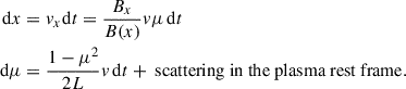 (A.4)
(A.4)
Scattering is done elastically in the plasma rest frame:
 (A.5)
(A.5)
where μn + 1 indicates the resulting pitch-angle cosine after scattering, μn the initial pitch-angle cosine before scattering,  with b = 2 ⋅ dt′⋅v′⋅γu/λ(x), where R1 ∈ [0, 1) is a sampled random number, dt′ the timestep in the plasma rest frame, dt′=(γ′/γ)dt, and γu the gamma factor related to the HTF speed, and ϕ = 2πR2, where R2 ∈ [0, 1) is another sampled random number.
The mean free path in the scattering process is taken to be proportional to the Larmor radius and spatially inversely proportional to the current:
 (A.6)
(A.6)
where p′=γ′mev′ is the momentum in the plasma frame, e is the elementary charge, and a ≥ 1 is a scaling constant.
We measure distances in the units of ion inertial length, di = VA/ωc, i = c/ωp, i, and speeds in the units of c. This means that time is measured in units of di/c. The dimensionless value of electron cyclotron frequency is
 (A.7)
(A.7)
where
 (A.8)
(A.8)
is a dimensionless property of the ambient medium, n1 is the ambient number density and  the magnitude of the ambient magnetic field. Thus, after fixing the value of α, the choice of the value of Bx becomes irrelevant, and we can take Bx ≃ 1 in the profiles, which means that
 (A.9)
(A.9)
and the hyperbolic cosine profile of the mean free path in dimensionless units becomes
 (A.10)
The equation of motion in the spatial dimension becomes
 (A.11)
Perpendicular magnetic field is compressed according to
 (A.12)
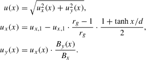
where MA is the Mach number in the HTF, so
![Mathematical equation: $$ \begin{aligned} \tan \theta _{Bn}(x)=\tan \theta _{Bn,1}\left[1+(r_{B\perp }-1)\cdot \frac{1+\tanh x/d}{2}\right], \end{aligned} $$](/articles/aa/full_html/2026/04/aa57951-25/aa57951-25-eq31.gif) (A.13)
(A.13)
similar to
![Mathematical equation: $$ \begin{aligned} u_{x}(x)=u_{x,1}\left[1-\frac{r_{g}-1}{r_{g}}\cdot \frac{1+\tanh x/d}{2}\right] \end{aligned} $$](/articles/aa/full_html/2026/04/aa57951-25/aa57951-25-eq32.gif) (A.14)
(A.14)
(At the limit of infinite Mach number, rB⊥ → rg.)
Finally,
![Mathematical equation: $$ \begin{aligned} \frac{1}{L}=-\frac{\tan \theta _{Bn}(x)}{[1+\tan ^{2}\theta _{Bn}(x)]^{3/2}}\frac{(r_{B\perp }-1)\tan \theta _{Bn,1}}{2d\cosh ^{2}x/d}. \end{aligned} $$](/articles/aa/full_html/2026/04/aa57951-25/aa57951-25-eq33.gif) (A.15)
(A.15)
Particles are injected from the upstream boundary of the simulation box, such that the pitch-angle cosine μ of each particle in the plasma rest frame allows it to enter the box and propagate toward the shock.
 (A.16)
where u is the upstream plasma flow speed in shock rest frame, v is the particle injection speed in the plasma rest frame, and R is a uniformly distributed random number such that all resulting pitch-angles propagate toward the shock at the edge of the simulation box.
Appendix B: Steady state result by integrating over time
The steady state of the particle distribution is indeed found by integrating the momentary particle distributions over time. Let us consider the focused transport equation (Wijsen 2020)
 (B.1)
(B.1)
where f is the particle distribution function, t is time (in HTF), s is distance measured along the field line, p is the particle momentum, μ is pitch-angle cosine, (δf/δt)turb implements the effects of turbulent fluctuations, Q is the particle source function, and δ the delta function. In a finite simulation box when t → ∞, the particle distribution function f → 0 as particles escape the box in a finite amount of time. Thus, integrating the above equation over time results in a steady state equation
 (B.2)
(B.2)
where F = ∫0∞fdt. Here we have assumed that the time derivatives and the turbulent scattering coefficients do not depend on time explicitly. The time integral of the distribution in our simulation corresponds to the binned distribution, where particles are incremented to the distribution after each time step weighed by the length of the time step in HTF.
Appendix C: Results for electron beam generation with a Maxwellian injection
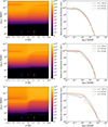 |
Fig. C.1. The reduced momentum distribution of particles propagating in the direction pointing from the downstream toward the upstream over position x in HTF reported in the units of energy for shock obliquities of 70°, 80°, and 85°. The right column displays energy spectra of slices taken from the reduced momentum distribution in the left column, correspondingly for each row at the positions specified by the color coded arrows. The mean free path profile λtrans is used. |
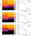 |
Fig. C.2. The reduced momentum distribution of particles propagating in the direction pointing from the downstream toward the upstream over position x in the HTF reported in the units of energy for shock obliquities of 86°, 87°, and 88°. The right column displays energy spectra of slices taken from the reduced momentum distribution in the left column, correspondingly for each row at the positions specified by the color coded arrows. The mean free path profile λtrans is used. |
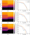 |
Fig. C.3. The reduced momentum distribution of particles propagating in the direction pointing from the downstream toward the upstream over position x in the HTF reported in the units of energy for shock obliquities of 86°, 87°, and 88°. The right column displays energy spectra of slices taken from the reduced momentum distribution in the left column, correspondingly for each row at the positions specified by the color coded arrows. The mean free path profile with the scaling factor of 10−4 is used. |
All Tables
All Figures
|
Fig. 1. Depiction of the 1D simulation model geometry in HTF. The singular spatial dimension of the model is along the shock normal, denoted as x. A finite-thickness shock is set at x = 0, with the upstream and downstream of the shock modeled with free-escape boundaries far from the shock. Particles travel along the magnetic field lines and particles’ position is tracked along x. Particle speed, v, pitch-angle cosine, μ, and residence time, t − t0, within the simulation box are also tracked. |
| In the text | |
|
Fig. 2. Zoom-in on the shock transition region of the simulation showcasing the local magnetic field obliquity, the local plasma flow speed in HTF, and the mean free path profile dependent on the gradient of the magnetic field with the input parameters of the simulation listed in Table 1. |
| In the text | |
|
Fig. 3. Particle energy spectrum in the plasma rest frame for escaping particle populations upstream and downstream of the shock for different minimum mean free paths at the shock. The box size used in the simulations corresponds to the injected particles’ diffusion length, Lbox ( = λ1vinjcos2θBn, 1/(3ux, 1) ≈ 3.5 ⋅ 105di), upstream and downstream of the shock along the magnetic field line. |
| In the text | |
|
Fig. 4. Particle energy spectrum in the plasma rest frame for escaping particle populations upstream and downstream of the shock for different minimum mean free paths at the shock. The box size used in the simulations is 20 di upstream and downstream of the shock along the magnetic field line. |
| In the text | |
|
Fig. 5. Depiction of the time-integrated phase space histogram of the simulation. As a particle spends a time step, dt, traveling between spatial histogram bins, the time spent in each bin, dt1 and dt2, is added to each respective bin. dt is set to be small enough for particles to not skip spatial bins when propagating through x. |
| In the text | |
|
Fig. 6. Time-integrated histogram as explained in Fig. 5 of particle positions zoomed in to the vicinity of the shock for the simulation box extending to the injected particles’ diffusion length upstream and downstream (top) and the simulation box extending to 20 di upstream and downstream (bottom) for different minimum mean free paths at the shock. |
| In the text | |
|
Fig. 7. Time-integrated phase space histogram of particles over particle position x and pitch-angle cosine μ in HTF for the simulation box extending to the injected particles’ diffusion length upstream and downstream for the λtrans mean free path profile (first from left), minimum mean free path factor of 10−4 (second from left), minimum mean free path factor of 10−5 (third from left), and minimum mean free path factor of 10−6 (fourth from left). |
| In the text | |
|
Fig. 8. Time-integrated phase space histogram of particles over particle position x and pitch-angle cosine μ in HTF for the simulation box extending to 20 di upstream and downstream for the λtrans mean free path profile (first from left), minimum mean free path factor of 10−4 (second from left), minimum mean free path factor of 10−5 (third from left), and minimum mean free path factor of 10−6 (fourth from left). |
| In the text | |
|
Fig. 9. Particle energy spectrum in the plasma rest frame for escaping particle populations upstream of the shock for shock obliquities 70°, 80°, and 85° (top) and 86°, 87°, and 88° (bottom). The box size used in the simulations corresponds to a 1 keV particle’s diffusion length upstream and downstream of the shock along the magnetic field line. The mean free path profile, λtrans, was used. |
| In the text | |
|
Fig. 10. Particle energy spectrum in the plasma rest frame for escaping particle populations downstream of the shock for shock obliquities 70°, 80°, and 85° (top) and 86°, 87°, and 88° (bottom). The box size used in the simulations corresponds to a 1 keV particle’s diffusion length upstream and downstream of the shock along the magnetic field line. The mean free path profile, λtrans, was used. |
| In the text | |
|
Fig. C.1. The reduced momentum distribution of particles propagating in the direction pointing from the downstream toward the upstream over position x in HTF reported in the units of energy for shock obliquities of 70°, 80°, and 85°. The right column displays energy spectra of slices taken from the reduced momentum distribution in the left column, correspondingly for each row at the positions specified by the color coded arrows. The mean free path profile λtrans is used. |
| In the text | |
|
Fig. C.2. The reduced momentum distribution of particles propagating in the direction pointing from the downstream toward the upstream over position x in the HTF reported in the units of energy for shock obliquities of 86°, 87°, and 88°. The right column displays energy spectra of slices taken from the reduced momentum distribution in the left column, correspondingly for each row at the positions specified by the color coded arrows. The mean free path profile λtrans is used. |
| In the text | |
|
Fig. C.3. The reduced momentum distribution of particles propagating in the direction pointing from the downstream toward the upstream over position x in the HTF reported in the units of energy for shock obliquities of 86°, 87°, and 88°. The right column displays energy spectra of slices taken from the reduced momentum distribution in the left column, correspondingly for each row at the positions specified by the color coded arrows. The mean free path profile with the scaling factor of 10−4 is used. |
| In the text | |
Current usage metrics show cumulative count of Article Views (full-text article views including HTML views, PDF and ePub downloads, according to the available data) and Abstracts Views on Vision4Press platform.
Data correspond to usage on the plateform after 2015. The current usage metrics is available 48-96 hours after online publication and is updated daily on week days.
Initial download of the metrics may take a while.