| Issue |
A&A
Volume 708, April 2026
|
|
|---|---|---|
| Article Number | A162 | |
| Number of page(s) | 10 | |
| Section | Planets, planetary systems, and small bodies | |
| DOI | https://doi.org/10.1051/0004-6361/202557980 | |
| Published online | 03 April 2026 | |
Apophis source population and Earth encounter frequency of Apophis-like bodies
1
Charles University, Faculty of Mathematics and Physics, Astronomical Institute, V Holešovičkách 2, 18000 Praha, Czech Republic
2
Department of Earth, Atmospheric and Planetary Sciences, MIT, 77 Massachusetts Avenue, Cambridge, MA 02139, USA
3
Aix-Marseille University, CNRS, CNES, LAM, Institut Origines, Marseille, France
4
European Southern Observatory (ESO), Karl-Schwarzschild-Strasse 2, 85748 Garching bei München, Germany
5
Trans-Tasman Occultation Alliance (TTOA), Wellington, PO Box 3181, New Zealand
★ Corresponding author: This email address is being protected from spambots. You need JavaScript enabled to view it.
Received:
4
November
2025
Accepted:
23
January
2026
Abstract
Context. Asteroid (99942) Apophis will safely pass by the Earth in April 2029. This extraordinary event will be observable by the naked eye from Africa and western Europe.
Aims. We provide context for the Apophis 2029 Earth passage by analyzing possible source populations for bodies in Apophis-like orbits, in particular, the Flora family, which has a mineralogical composition corresponding to LL chondrite meteorites, similar to measurements of Apophis itself.
Methods. We estimated the specific encounter probability of the present-day orbit of Apophis by classical Öpik and N-body methods. We then performed orbital simulations of the Flora family, initializing bodies between 2.1 and 2.3 au, and tracked their evolution into the near-Earth object (NEO) space to compute their mean and peak encounter probabilities with Earth.
Results. Out of an estimated population of ~3380 NEOs larger than or equal to Apophis (≥420 m), 610 ± 140 are LL-like NEOs from Flora. Their mean encounter probability is p = 86 × 10−18 km−2 yr−1, corresponding to a once per 13 000 y frequency of encounters closer than 38 000 km. However, this does not apply to Apophis alone, for which the specific encounter probability is higher p′ = 1603 × 10−18 km−2 yr−1, but the frequency is lower, only once per 430 000 y, when we consider it as a single object. Our simulation of the Flora family over ~1 billion years indicates that Apophis-like bodies from Flora have orbits that are particularly persistent in nearEarth space. The temporal distribution of encounter probabilities exhibits peaks (up to >104 in the same units) and the specific value for Apophis is not unusual (occurring ~70% of time). In other words, there is always at least one Apophis-like body among NEOs. We find that such persistence also creates favorable opportunities for temporary capture as Earth coorbitals and Apophis-like bodies are ultimately removed from the inner Solar System by approaching the Sun or by impact into one of the terrestrial planets, where the relative split between these outcomes is (45 ± 2)% and (50 ± 2)%. While our current knowledge of the Apophis orbit guarantees no threat from Apophis in the next few centuries, we cannot predict any specific outcome for Apophis in the coming thousands or millions of years. Evaluating this statistically over the long term, we find that objects in Apophis-like orbits have a (19 ± 2)% chance of Earth impact over their lifetime of ~30Myr.
Conclusions. Apophis appears to be a prototypical example for the population of hundred-meter bodies intersecting Earth’s orbit and impacting the Earth, making it a particularly worthwhile target for investigations, thus advancing our knowledge for planetary defence.
Key words: ephemerides / occultations / Earth / minor planets, asteroids: individual: (99942) Apophis / minor planets, asteroids: individual: (3753) Cruithne
© The Authors 2026
 Open Access article, published by EDP Sciences, under the terms of the Creative Commons Attribution License (https://creativecommons.org/licenses/by/4.0), which permits unrestricted use, distribution, and reproduction in any medium, provided the original work is properly cited.
This article is published in open access under the Subscribe to Open model. This email address is being protected from spambots. You need JavaScript enabled to view it. to support open access publication.
1 Introduction
The asteroid (99942) Apophis is one of the near-Earth objects (NEOs) that regularly undergoes close encounters with the Earth. In this specific case, however, one of the encounters will be particularly close, on Friday 13 April 2029 (Giorgini et al. 2008), which explains its status as a high-profile target for ongoing observational campaigns (Farnocchia et al. 2013; Vokrouhlický et al. 2015; Souchay et al. 2018; Brozović et al. 2018; Binzel et al. 2021; Reddy et al. 2022) and also for upcoming in situ measurements (Polit et al. 2024; Martino et al. 2024).
Given the importance of Apophis for planetary science and for planetary defence, it is important to provide the corresponding context, in terms of the overall NEO population. The questions we would like answers to are whether Apophis is exceptional, whether the 2029 Apophis close encounter is truly rare, where Apophis most likely originated from, and whether there are any other bodies among NEOs that can become - on a long timescale - Apophis-like. We address these questions in this contribution.
The current osculating orbit of Apophis (a = 0.9227 au, e = 0.1914, i = 3.339°) corresponds to a deep Earth-crosser that is detached from the belt between Mars and Jupiter. Integrating its orbit backward in time and finding its origin within the belt is impossible for multiple reasons (e.g., deterministic chaos, diffusion, dissipative forces, collisions, S = k. log W). Nevertheless, most of the currently discovered NEOs are believed to originate from the Flora family, located at the inner edge of the belt (Vernazza et al. 2008; Marsset et al. 2024; Brož et al. 2024a,b; Lagain et al. 2025). This link is consistent with global modeling of transport from the belt and with mineralogical classification of families and NEOs. Specifically, their mineralogy corresponds to LL chondrite meteorites. Spectral observations of Apophis also correspond to LL-like mineralogy (Binzel et al. 2009; Reddy et al. 2018), so linking Apophis to Flora seems to be consistent compositionally as well as dynamically.
2 Results
2.1 Probability of coming from a source
As a first step, we quantified the probabilities that Apophis comes from each of several relevant sources in the belt. We used the METEOMOD/NEOMOD model1 from Brož et al. (2024a); Lagain et al. (2025), which is based on an extensive set of 56 asteroid families. For subkilometer-sized NEOs only families are relevant because the background population is depleted due to the low strength of subkilometer bodies (Benz & Asphaug 1999; Bottke et al. 2005, 2020) and collisional cascade, as confirmed by recent James Webb Space Telescope observations (Burdanov et al. 2025). For each family, its synthetic size-frequency distribution (SFD), Nmb(>D), is constrained by the observed SFD and extrapolated to smaller sizes below the observational limit. This extrapolation is not simplified (power law), but is based on a dedicated collisional model. Then, the corresponding NEO population is estimated as
 (1)
(1)
where the two dynamical timescales correspond to the mean lifetimes of synthetic orbits in the belt and in the NEO space. Our removal criteria were q < R⊙, r > 100 au (for more details, see Brož et al. 2024a).
In order to estimate the source probability starting with any specific NEO orbit, it turns out that the semimajor axis a and inclination i are better indicators than the orbital eccentricity e, because e undergoes the greatest alteration. (the value of e must be substantially increased as a prerequisite for it to enter nearEarth space.) Hence, binned distributions Mj(a, i) of synthetic NEO orbits, originating from individual families, were used to compute the probability of coming from a source j as
 (2)
(2)
and the sum Σjpj was re-normalized, assuming there is no other mysterious source.
If we use all families, regardless of their mineralogical composition, and assume D = 1 km for simplicity, we obtain the highest probability for Flora (~0.52), followed by Polana (0.29), Nysa (0.09), Juno (0.04), and Vesta (0.04). Generally, these are the families that contribute most to the kilometer-size NEO population and, simultaneously, produce objects on Apophis-like orbits. We formally define Apophis-like bodies as NEOs that have perihelion q < 1.016 au, aphelion Q > 0.983 au, and a < 1.523 au; that experience at least five close encounters (<0.01 au) with Earth per 104 years; and that have a dynamical lifetime τneo > 10Myr (Fig. B.2).
Mineralogical composition provides an additional constraint on the source population of Apophis. Since it is spectroscopically analogous to LL chondrite meteorites, we restricted our search to the subset of LL-like source regions identified by Vernazza et al. (2008); Marsset et al. (2024). These include only three major asteroid families, Flora, Eunomia, and a part of Nysa, since another part of Nysa is either too dark (M type) or too bright (E type). We also considered the Juno family, whose members are mostly identified compositionally as L/LL (Marsset et al. 2024). The resulting probabilities are summarized in Table 1. Only Flora, Nysa, and Juno produced some Apophis-like orbits; Eunomia is located a bit too far beyond the 3:1 mean-motion resonance with Jupiter (see Figs. 1 and D.1). Furthermore, Flora (with ~0.86 probability) dominates other sources, not only because Flora family members are so numerous, but it is also the best-positioned source, due to the proximity of the ν6 secular resonance (Vokrouhlický et al. 2017) and the relatively strong influence of the Yarkovsky effect at the inner edge of the asteroid belt at 2.1 au (Vokrouhlický & Farinella 1999).
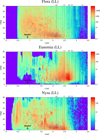 |
Fig. 1 Binned distributions Mj of semimajor axes a and inclinations i of synthetic NEO orbits, originating from individual asteroid families. The colors correspond to the number of test particles in bins, although the quantity Mj(a, i) was eventually normalized. The bin sizes were 0.01 au and 1°, respectively. The Apophis orbit is marked with a black cross. The orbits of other LL-like NEOs from Binzel et al. (2019); Marsset et al. (2022) are marked with gray crosses. Of the three, the highest density for producing Apophis-like objects is from the Flora family. |
2.2 Mean encounter frequency for Apophis
In order to estimate the mean encounter frequency for Apophis, one needs to know its size, because the population is sizedependent. Unfortunately, there is a tangible disagreement between the volume-equivalent diameters 340 m from radar (Brozović et al. 2018) versus 380 m from infrared observations (Müller et al. 2014) versus 420 m from occultations (Appendix C). Hereafter, we prefer the latter, since occultations are less prone to calibration or systematic uncertainties, provided the respective occultation event was not too short, cadence of measurements not too long or that diffraction patterns were taken into consideration (e.g., Brož & Wolf 2021).
The cumulative number of bodies Nmb in the Flora family, which are larger than 420 m, was extrapolated from the observed size distribution using a collisional model of Brož et al. (2024a); Lagain et al. (2025). The equilibrium NEO population originating from Flora was estimated again from Eq. (1). For Nmb = 21 000 ± 2000, τneo = (9.95 ± 0.5)Myr, and Tmb = (340 ± 30)Myr, we obtained Nneo = 610 ± 140. The uncertainty of this estimate is mostly due to stochasticity of the collisional model at subkilometer sizes.
We estimated the corresponding collisional probabilities of these bodies and the frequency of encounters with the Earth. From our N -body simulations of transport from Flora (Brož et al. 2024a; Lagain et al. 2025), the intrinsic scaled collisional probability of NEOs is
 (3)
(3)
hence the flux
 (4)
(4)
and the number of encounters
 (5)
(5)
where we used Nneo as the number of pairs (since Earth is just one). If we assume the geocentric distance R = 38 000 km, the interval is approximately ∆t = (13 000 ± 3500) yr, in order to get Nenc = 1. This is a longer mean interval than the 7500 y value from Farnocchia & Chodas (2021); Nesvorný et al. (2024) because here we assumed a specific subpopulation of LL-like NEOs from Flora.
We wondered if this makes the 2029 Apophis encounter an even greater rarity than previously calculated. We decided that it did not, because the value above is a characteristic of the NEO population, not of Apophis alone. Before answering the question, one needs to know three things: (i) the specific collisional probability for Apophis; (ii) the long-term evolution of Apophis’ orbit; (iii) the encounter frequencies for Apophis-like bodies.
Source probabilities from five asteroid families (including three dominated by LL compositions) for delivering objects into Apophis-like orbits.
2.3 Specific encounter frequency for Apophis
If the current, osculating orbit of Apophis is used to compute its collisional probability with the Öpik theory (Öpik 1951; Bottke & Greenberg 1993), one obtains
 (6)
(6)
This is almost 20 times more than p above (Eq. (3)), a confirmation that Apophis orbit is exceptional, at the current epoch, compared to other, ordinary NEOs. If we focus on Apophis alone (Nneo = 1), its specific single-body encounter frequency would be as long as once per 430 000 yr.
We note that the Öpik theory assumes a uniform precession of angles (ω, Ω), which is a good approximation of short-term orbital evolution, provided the orbits of colliding bodies are uncorrelated. This is most likely the case for old families and most NEOs (but not for young families; Vokrouhlický et al. 2021). Of course, for the ephemerides and deterministic predictions of encounters (e.g., 2029, 2036, 2068), this is not a suitable theory, but here we are interested in statistics of encounters.
2.4 Long-term evolution of the Apophis orbit
We also computed the long-term evolution of clones having Apophis-like orbits, using a standard N-body model (Levison & Duncan 1994; Brož et al. 2011). We employed the symplectic integrator RMVS3, which handles close encounters with planets by subdividing the time step. We included gravitational perturbations by planets from Mercury to Neptune, Ceres, Vesta, the Yarkovsky effect, the YORP effect; assuming simplified, principal-axis rotation, with the period P = 30.56 h, but not tumbling (Pravec et al. 2014; Lee et al. 2022), which is an acceptable approximation (Vokrouhlický et al. 2015). The respective thermal parameters correspond to S-type bodies covered by regolith, the bulk density ρ = 2000 kg m−3, the conductivity K = 0.07Wm−1 K−1, and the capacity C = 680Jkg−1 K−1, the Bond albedo A = 0.14, the emissivity ε = 0.86. The diurnal drifts ȧ then span a range ±0.0015 au Myr−1 for various obliquities. For comparison, the actual astrometric measurement of the Yarkovsky drift for Apophis is within this range: ȧ = (-0.00133 ± 0.00001) auMyr−1 (Pérez-Hernández & Benet 2022; Farnocchia & Chesley 2022).
We used 100 clones of Apophis, with various obliquities. The time step was 0.9 d, the output time step δt = 103 yr, and the overall time span ∆t ≥ 10Myr, in order to obtain the statistical distribution of up to 106 sets of osculating orbital elements shown in Fig. 2. We computed the collisional probability for this sample and obtained
 (7)
(7)
This is still almost an order of magnitude more than p above (Eq. (3)); a confirmation that the Apophis orbit is exceptional, even over its long-term evolution. We find that objects in Apophis-like orbits spend more time with a higher average collisional probability when compared to other NEOs. We note that the value is temporally dependent as p" (t) tends to decrease as an Apophis-like orbit evolves across the NEO space.
Moreover, the dynamical lifetime of some orbits is up to 100 Myr (Fig. 2, bottom). The clones were eliminated slowly, on an e-folding timescale of ~30 Myr, often by being too close to the Sun or by planetary impacts. This is again above the average ~8 Myr (Granvik et al. 2016, 2018). The reason is that at moderate inclinations of at least few degrees, and not crossing any other terrestrial planets (q = 0.7460 au, Q = 1.0993 au), collisional probabilities decrease and an NEO orbit can survive for a long time. In other words, we find that on average, objects in Apophis-like orbits persist longer than most other objects in near-Earth space.
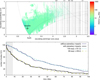 |
Fig. 2 Top: osculating semimajor axis a vs. eccentricity e showing long-term evolution of Apophis-like orbits, after 10Myr. The curves correspond to the boundaries of the NEO space (q < 1.3 au, Q > 0.983 au) and of the adjacent Mars-crossing population. The dotted vertical lines correspond to locations of various mean-motion resonances, including the ν6 secular resonance. The majority of the 100 clones of Apophis remain in the NEO (or Mars-crossing) space; the respective orbit is relatively long-lived. Bottom: number of Apophis clones N vs. time t. The corresponding e-folding timescale is -30 Myr or 50 Myr, respectively, depending on whether or not planetary impacts were used as a criterion for the removal of bodies. |
2.5 Peak encounter frequency for Apophis-like bodies
As far as Apophis-like bodies are concerned (cf. Fig. B.2), these clearly originate from the Flora family. We thus took the synthetic Flora family from Brož et al. (2024a); Lagain et al. (2025) and analyzed the orbital distribution of the corresponding synthetic NEOs. Since the age of the Flora family is (1.3 ± 0.1) Gy, in the past it supplied substantially more objects to the NEO population than today (Vokrouhlický et al. 2017; Lagain et al. 2025). In our simulation, we started with an arbitrary, representative sample of ~1900 test particles and their number decreased slowly and exponentially in the course of time.
Out of these, one can distinguish short- and long-lived orbits (their mix determines the mean lifetime τneo ). The actual lifetimes of individual bodies are diverse, ranging from <0.1 to hundreds of megayears (see Fig. 3). This is closely related to collisional probabilities, which are also diverse, from zero (if orbits do not intersect the Earth) up to >104, in the 10−18 km−2 yr−1 units (see Fig. 4). Such peaks are common and there are intervals of time for which at least one Apophis-like body is statistically present among NEOs throughout the entire duration of our simulation.
Finally, we must take into account that the actual number of bodies larger than 420 m is higher than in our simulation. Since the peaks in probabilities are randomly distributed in time, one can simply use a Monte Carlo approach: draw a sample of Nneo = 610 from all p values, determine its maximum p value, and repeat to obtain the respective distribution. According to Fig. 4 (bottom), there is a -70% chance of having at least one Apophis-like body in the population of LL-like NEOs.
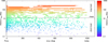 |
Fig. 3 Lifetimes of LL-like NEOs originating from the Flora family according to our simulation. The x-axis is simulation time (spanning from 0, i.e., Flora disruption, to 1 Gy, the end of simulation); the y-axis is lifetime. One can see both short-lived orbits (blue) and long-lived orbits (orange); their mix determines the mean lifetime τneo. |
2.6 The fate of (99942) Apophis
More than two decades of orbital tracking, including high-precision radar position and velocity measurements, conclusively show that Apophis poses absolutely no threat to Earth in the coming few centuries (Farnocchia & Chesley 2022; Brozović et al. 2022; Chesley & Farnocchia 2023; Dotson et al. 2023). Nevertheless, the ultimate fate of Apophis in a forecast of thousands or millions of years is unknown.
To evaluate the statistical possibilities in a long-term Apophis forecast, we used our long-term orbital simulations (Sects. 2.4 and 2.5) to understand the fate of bodies on Apophis-like orbits. We evaluated the outcomes of Apophis clones by considering their statistical removal from the inner Solar System through close intersections or collisions with the Sun, Mercury, Venus, Earth, and Mars (Fig. 5). It turned out that over the typical 30 million-year lifetime for an Apophis clone, approximately (45 ± 2)% of the clones were eliminated due to low perihelion (q < R⊙), and (50 ± 2)% due to planetary impacts. Out of those, Earth and Venus were the most effective planets since they have the most sizeable cross sections and focussing factors. Such increased probabilities of planetary impacts were previously reported for some special NEOs, for example ejecta from the Moon-forming impact (Bottke et al. 2014), space debris (Rein et al. 2018), or Eros (Michel et al. 1998). This is very different from other ordinary NEOs, which mostly collide with the Sun; only ~1% of them impact the Earth (Fig. D.2).
Our findings thus reveal the particular importance of objects in Apophis-like orbits for evaluating the non-negligible longterm impact hazard to Earth. Most profoundly, they indicate the scientific study opportunity presented by the 2029 close passage by Apophis is particularly valuable toward advancing our knowledge in the applied science of planetary defence.
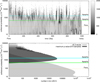 |
Fig. 4 Top: collisional probabilities of LL-like NEOs originating from the Flora family and their temporal distribution. Individual bodies (out of 1900) are distinguished by shades of gray. The vertical range shows both low and high probabilities. For comparison, the horizontal lines indicate the mean probability p of all NEOs (orange), short-term initial probability p′ of Apophis (cyan), long-term probability p″ of Apophis (green). Bottom: Distribution of all p values (gray) and of the maximum p value (black). |
3 Discussion
Another implication of our long-term evaluation of Apophis-like orbits is considering the frequency with which such objects may pass by the Earth at a near-miss distance inside the Roche limit.
3.1 Passages within the Roche limit
We thus computed the frequency of passages within the Roche limit. Specifically, for Apophis-like objects:
 (8)
(8)
Here we used ρ = 2000 kg m−3 (Vokrouhlickÿ et al. 2015); the coefficient k ≈ 2 suitable for rubble piles is lower than for fluids (Leinhardt et al. 2012; Zhang & Michel 2020). Since we already know the frequency of R ≥ 38 000 km encounters (Sect. 2.3), the surface area ratio is (Rroche/R)2 = 0.22, the frequency of Rochelimit encounters is once per 1.9 Myr. However, this is a relatively long time and the long-term collisional probability p″ (Eq. (7)) is lower, which shifts the estimate to once per 6.9 Myr. Consequently, it is possible that Apophis has undergone in the past, or will undergo in the future, several Roche-limit passages over the course of its lifetime (~30Myr) as a near-Earth object. The nonzero number (~3-7) of Roche-limit passages is important for the interpretation of in situ observations.
Such passages make asteroid surfaces look fresher, or Q type (Binzel et al. 2010; Nesvornÿ et al. 2010). Surface refreshment may come from seismic shaking during the encounter or from subsequent long-term re-equilibration after finding itself in a tidally torqued new spin state (Ballouz et al. 2024). At the same time, however, these orbits often exhibit low perihelia, which lead to the thermal processing of the regolith (Delbo et al. 2014; Graves et al. 2019). Apophis itself has a weathered, transitional, Sq-type spectrum (Binzel et al. 2009), between S and Q, which is an indication of a relatively long (>1 Myr) interval from the last resurfacing event.
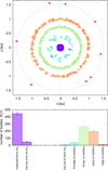 |
Fig. 5 Top: collisions of Apophis clones with the Sun, Mercury, Venus, Earth, or Mars. Their positions in the ecliptic frame (x, y) are indicated (crosses), alongside the mean orbital distances of terrestrial planets (dotted circles). Bottom: statistics of collisions. Specifically, (45 ± 2)% of the clones were eliminated due to low perihelion (q < R⊙), while (50 ± 2)% due to planetary impacts. The respective uncertainties (error bars) are Poissonian (∝ √N). |
3.2 Relation to temporary coorbitals
In order to understand possible relation of Apophis-like bodies to other NEO populations, we also checked how often they become Earth coorbitals (Wiegert et al. 2000; Christou 2000). According to the long-term evolution of Apophis clones (Sect. 2.4), 415 out of 1000 bodies were temporarily located in the coorbital region (a ∈ (0.995; 1.005) au, e ≲ 0.2). Some captures were short (≤103 yr, i.e., corresponding to our sampling), but we also noticed ten long-term captures, spanning one or more megayears (see Fig. 6). They orbited on horseshoe orbits, which is the most common type (Kaplan & Cengiz 2020). The percentage of time Apophis clones spent in this region is on the order of 0.5 ± 0.1%. For comparison, all NEOs larger than 420 m would spend only 0.02% as coorbitals because, on average, they do not orbit so close to the Earth. An implication is that Apophis-like bodies are the most likely source of Earth coorbitals.
Another question we have asked is where else the Earth’s coorbitals could come from. It must be from within the NEO region because an object cannot be injected into the coorbital region without temporarily being a NEO. Moreover, the respective mechanism must provide sufficient ∆v, for example close encounters with the Earth (or Venus), which again points to Apophis-like bodies2.
This is in agreement with spectral observations of (3753) Cruithne (Angeli & Lazzaro 2002; de León et al. 2010), the only known kilometer-sized Earth coorbital (Usui et al. 2011). Cruithne itself does not qualify as Apophis-like by our criteria as it currently experiences no close encounters with Earth, despite its coorbital configuration. Nevertheless, it is classified as Q type, suggesting a relatively recent (<1Myr) resurfacing (Sect. 3.1). We determined the mineralogical composition of Cruithne from its reflectance spectrum (Binzel et al. 2019; Marsset et al. 2022), using the Brunetto et al. (2006) and Shkuratov et al. (1999) models for reddening and reflection, respectively (Fig. 7). The ratio of olivine to orthopyroxene, ol/(ol+opx) = 0.755, corresponds to LL-like composition, fully compatible with the Flora family origin (cf. Marsset et al. 2024, Fig. 1).
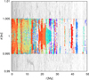 |
Fig. 6 Osculating semimajor axis a vs. time t for Apophis clones. When bodies were located within the coorbital region of the Earth (a ∈ (0.995; 1.005) au), e < 0.2), they were plotted in color to distinguish individual bodies, otherwise in gray. |
4 Conclusions
We reached a similar rarity of once per ~4700 years as Farnocchia & Chodas (2021) for the 2029 close passage by (99942) Apophis (see Appendices A, B and Table 2), and we find that the Flora family is rather prolific as the progenitor for such encounters by LL-like NEOs, orbiting on relatively long-lived (~30Myr) orbits in Earth’s vicinity. While Apophis-like bodies represent only ~3% of the NEO population larger than 420 m, they are responsible for approximately half of all close Earth encounters. Apophis, as a prototypical example, will end its journey (i) by being removed by the Earth or Venus, or slightly less likely, (ii) by approaching too close to the Sun. An implication is that these bodies pass several times within the Roche limit and because their orbits are so similar to the Earth’s, they are also related to temporary coorbitals. Flora will nonetheless continue to contribute additional NEOs, which will undergo deep close encounters with planets. This behavior is clearly seen in our simulations of the Flora family.
If considering Apophis alone, it should be noted that its encounter frequency with Earth is once per ~430 000yr. It is very, very rare because it was computed for a single body and for a close encounter within the geocentric distance R = 38 000 km.
If considering LL-like NEOs, originating from the Flora family, their encounter frequency is once per ~ 13 000 yr. Only if one considers all NEOs, regardless of their mineralogy, is the frequency once per ~4700 yr.
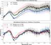 |
Fig. 7 Top: observed mean reflectance spectrum of Apophis and Cruithne from the MITHNEOS survey (Binzel et al. 2019; Marsset et al. 2022). Their comparison to taxonomic classes (S, Sq, Q) shows that Apophis is Sq type and Cruithne is Q type. Bottom: same spectra after dereddening (Brunetto et al. 2006); we note the applicability in the visible of this simplified, exp(-CS/λ) model is limited. Their comparison to ordinary chondrite classes (H, L, LL) shows that both asteroids are LL-like. |
Estimates of populations Nmb(>D), Nneo(>D), and encounter frequencies ∆t for Apophis itself, LL-like NEOs from Flora, and all NEOs.
Acknowledgements
M.B. was supported by GACR grant no. 25-16789S of the Czech Science Foundation. J.D. was supported by GACR grant no. 23-04946S of the Czech Science Foundation. The work of O.C. was supported by the Czech Science Foundation (grant 25-16507S), the Charles University Research Centre program (No. UNCE/24/SCI/005), and the Ministry of Education, Youth and Sports of the Czech Republic through the e-INFRA CZ (ID: 90254). We thank an anonymous referee for their insightful comments.
References
- Angeli, C. A., & Lazzaro, D. 2002, A&A, 391, 757 [NASA ADS] [CrossRef] [EDP Sciences] [Google Scholar]
- Ballouz, R.-L., Agrusa, H., Barnouin, O. S., et al. 2024, Planet. Sci. J., 5, 251 [Google Scholar]
- Benz, W., & Asphaug, E. 1999, Icarus, 142, 5 [NASA ADS] [CrossRef] [Google Scholar]
- Binzel, R. P., Rivkin, A. S., Thomas, C. A., et al. 2009, Icarus, 200, 480 [NASA ADS] [CrossRef] [Google Scholar]
- Binzel, R. P., Morbidelli, A., Merouane, S., et al. 2010, Nature, 463, 331 [NASA ADS] [CrossRef] [Google Scholar]
- Binzel, R. P., DeMeo, F. E., Turtelboom, E. V., et al. 2019, Icarus, 324, 41 [Google Scholar]
- Binzel, R., Barbee, B. W., Barnouin, O. S., et al. 2021, in Bulletin of the American Astronomical Society, 53, 045 [Google Scholar]
- Bottke, W. F., & Greenberg, R. 1993, Geophys. Res. Lett., 20, 879 [Google Scholar]
- Bottke, W. F., Durda, D. D., Nesvorný, D., et al. 2005, Icarus, 175, 111 [Google Scholar]
- Bottke, W. F., Vokrouhlický, D., Marchi, S., et al. 2014, in 45th Annual Lunar and Planetary Science Conference, Lunar and Planetary Science Conference, 1611 [Google Scholar]
- Bottke, W. F., Vokrouhlický, D., Ballouz, R. L., et al. 2020, AJ, 160, 14 [Google Scholar]
- Brož, M., & Wolf, M. 2021, Astronomická měření (Matfyzpress) [Google Scholar]
- Brož, M., Vokrouhlický, D., Morbidelli, A., Nesvorný, D., & Bottke, W. F. 2011, MNRAS, 414, 2716 [Google Scholar]
- Brož, M., Vernazza, P., Marsset, M., et al. 2024a, A&A, 689, A183 [NASA ADS] [CrossRef] [EDP Sciences] [Google Scholar]
- Brož, M., Vernazza, P., Marsset, M., et al. 2024b, Nature, 634, 566 [Google Scholar]
- Brozović, M., Benner, L. A. M., McMichael, J. G., et al. 2018, Icarus, 300, 115 [CrossRef] [Google Scholar]
- Brozović, M., Benner, L. A. M., Naidu, S. P., et al. 2022, in LPI Contributions, 2681, Apophis T-7 Years: Knowledge Opportunities for the Science of Planetary Defense, 2023 [Google Scholar]
- Brunetto, R., Vernazza, P., Marchi, S., et al. 2006, Icarus, 184, 327 [CrossRef] [Google Scholar]
- Burdanov, A. Y., de Wit, J., Brož, M., et al. 2025, Nature, 638, 74 [Google Scholar]
- Chesley, S. R., & Farnocchia, D. 2023, in LPI Contributions, 2988, Apophis T-6 Years: Knowledge Opportunities for the Science of Planetary Defense, 2031 [Google Scholar]
- Christou, A. A. 2000, Icarus, 144, 1 [NASA ADS] [CrossRef] [Google Scholar]
- de León, J., Licandro, J., Serra-Ricart, M., Pinilla-Alonso, N., & Campins, H. 2010, A&A, 517, A23 [CrossRef] [EDP Sciences] [Google Scholar]
- Delbo, M., Libourel, G., Wilkerson, J., et al. 2014, Nature, 508, 233 [Google Scholar]
- Dotson, J. L., Brozović, M., Chesley, S., et al. 2023, in LPI Contributions, 2988, Apophis T-6 Years: Knowledge Opportunities for the Science of Planetary Defense, 2035 [Google Scholar]
- Ďurech, J., Kaasalainen, M., Herald, D., et al. 2011, Icarus, 214, 652 [Google Scholar]
- Ďurech, J., Ortiz, J. L., Ferrais, M., et al. 2025, A&A, 696, A76 [NASA ADS] [CrossRef] [EDP Sciences] [Google Scholar]
- Ďurech, J., Vokrouhlický, D., Pravec, P., et al. 2026, A&A, submitted [Google Scholar]
- Farnocchia, D., & Chodas, P. W. 2021, RNAAS, 5, 257 [Google Scholar]
- Farnocchia, D., & Chesley, S. R. 2022, in LPI Contributions, 2681, Apophis T-7 Years: Knowledge Opportunities for the Science of Planetary Defense, 2007 [Google Scholar]
- Farnocchia, D., Chesley, S. R., Chodas, P. W., et al. 2013, Icarus, 224, 192 [Google Scholar]
- Giorgini, J. D., Benner, L. A. M., Ostro, S. J., Nolan, M. C., & Busch, M. W. 2008, Icarus, 193, 1 [NASA ADS] [CrossRef] [Google Scholar]
- Granvik, M., Morbidelli, A., Jedicke, R., et al. 2016, Nature, 530, 303 [Google Scholar]
- Granvik, M., Morbidelli, A., Jedicke, R., et al. 2018, Icarus, 312, 181 [CrossRef] [Google Scholar]
- Graves, K. J., Minton, D. A., Molaro, J. L., & Hirabayashi, M. 2019, Icarus, 322, 1 [NASA ADS] [CrossRef] [Google Scholar]
- Herald, D., Gault, D., Carlson, N., et al. 2024, Small Bodies Occultations Bundle V4.0, NASA Planetary Data System, urn:nasa:pds:smallbodiesoccultations::4.0 [Google Scholar]
- Jiao, Y., Cheng, B., Huang, Y., et al. 2024, Nat. Astron., 8, 819 [NASA ADS] [CrossRef] [Google Scholar]
- Kaplan, M., & Cengiz, S. 2020, MNRAS, 496, 4420 [NASA ADS] [CrossRef] [Google Scholar]
- Lagain, A., Brož, M., Fairweather, J., et al. 2025, Nature, submitted [Google Scholar]
- Lee, H. J., Kim, M. J., Marciniak, A., et al. 2022, A&A, 661, L3 [NASA ADS] [CrossRef] [EDP Sciences] [Google Scholar]
- Leinhardt, Z. M., Ogilvie, G. I., Latter, H. N., & Kokubo, E. 2012, MNRAS, 424, 1419 [NASA ADS] [CrossRef] [Google Scholar]
- Levison, H. F., & Duncan, M. J. 1994, Icarus, 108, 18 [NASA ADS] [CrossRef] [Google Scholar]
- Mainzer, A., Grav, T., Bauer, J., et al. 2011, ApJ, 743, 156 [NASA ADS] [CrossRef] [Google Scholar]
- Marsset, M., DeMeo, F. E., Burt, B., et al. 2022, AJ, 163, 165 [NASA ADS] [CrossRef] [Google Scholar]
- Marsset, M., Vernazza, P., Brož, M., et al. 2024, Nature, 634, 561 [Google Scholar]
- Martino, P., Michel, P., Küppers, M., & Carnelli, I. 2024, in 45th COSPAR Scientific Assembly, 45, 241 [Google Scholar]
- Michel, P., Farinella, P., & Froeschlé, C. 1998, AJ, 116, 2023 [Google Scholar]
- Moskovitz, N. A., Wasserman, L., Burt, B., et al. 2022, Astron. Comput., 41, 100661 [NASA ADS] [CrossRef] [Google Scholar]
- Müller, T. G., Kiss, C., Scheirich, P., et al. 2014, A&A, 566, A22 [NASA ADS] [CrossRef] [EDP Sciences] [Google Scholar]
- Nesvorný, D., Bottke, W. F., Vokrouhlický, D., Chapman, C. R., & Rafkin, S. 2010, Icarus, 209, 510 [CrossRef] [Google Scholar]
- Nesvorný, D., Vokrouhlický, D., Shelly, F., et al. 2024, Icarus, 417, 116110 [Google Scholar]
- Öpik, E. J. 1951, Pattern Recogn. Image Anal., 54, 165 [Google Scholar]
- Pérez-Hernández, J. A., & Benet, L. 2022, Commun. Earth Environ., 3, 10 [Google Scholar]
- Polit, A., DellaGiustina, D., Nolan, M., et al. 2024, in 45th COSPAR Scientific Assembly, 45, 242 [Google Scholar]
- Pravec, P., Scheirich, P., Ďurech, J., et al. 2014, Icarus, 233, 48 [NASA ADS] [CrossRef] [Google Scholar]
- Reddy, V., Sanchez, J. A., Furfaro, R., et al. 2018, AJ, 155, 140 [NASA ADS] [CrossRef] [Google Scholar]
- Reddy, V., Kelley, M. S., Dotson, J., et al. 2022, Planet. Sci. J., 3, 123 [NASA ADS] [CrossRef] [Google Scholar]
- Rein, H., Tamayo, D., & Vokrouhlický, D. 2018, Aerospace, 5, 57 [Google Scholar]
- Shkuratov, Y., Starukhina, L., Hoffmann, H., & Arnold, G. 1999, Icarus, 137, 235 [Google Scholar]
- Souchay, J., Lhotka, C., Heron, G., et al. 2018, A&A, 617, A74 [NASA ADS] [CrossRef] [EDP Sciences] [Google Scholar]
- Usui, F., Kuroda, D., Müller, T. G., et al. 2011, PASJ, 63, 1117 [Google Scholar]
- Vernazza, P., Binzel, R. P., Thomas, C. A., et al. 2008, Nature, 454, 858 [NASA ADS] [CrossRef] [Google Scholar]
- Vokrouhlický, D., & Farinella, P. 1999, AJ, 118, 3049 [CrossRef] [Google Scholar]
- Vokrouhlický, D., Farnocchia, D., Capek, D., et al. 2015, Icarus, 252, 277 [CrossRef] [Google Scholar]
- Vokrouhlický, D., Bottke, W. F., & Nesvorný, D. 2017, AJ, 153, 172 [Google Scholar]
- Vokrouhlický, D., Brož, M., Novaković, B., & Nesvorný, D. 2021, A&A, 654, A75 [NASA ADS] [CrossRef] [EDP Sciences] [Google Scholar]
- Wiegert, P., Innanen, K., & Mikkola, S. 2000, Icarus, 145, 33 [Google Scholar]
- Zhang, Y., & Michel, P. 2020, A&A, 640, A102 [NASA ADS] [CrossRef] [EDP Sciences] [Google Scholar]
Appendix A Comparison to Farnocchia & Chodas (2021)
If we use the Öpik theory and apply it to all NEOs larger than 420 m, we obtain the NEO population Nneo = 3380 ± 300 (Nesvorný et al. 2024), the probability p′″ = (44.311 ± 3) × 10−18km−2y−1, the flux Φ = (1.5 ± 0.2) × 10−13km−2y−1, and the corresponding frequency once per (4620 ± 720) y.
Our value is in modest disagreement with Farnocchia & Chodas (2021), who reported once per 7500 y. The non-negligible difference between the values is due to several factors: (i) they used the absolute magnitude limit (H = 19.1 mag); (ii) their population was 10% lower (Nneo(<H) = 3025); (iii) they used the mean, per-object impact probability p 1 = 1.66 × 10⁻⁹y−1, equivalent to  ; (iv) their gravitational focussing was obtained as an integration over the velocity distribution. This is different from our, more precise approach, because we used a per-object impact velocity (Bottke & Greenberg 1993), hence per-object gravitational focussing, which is correlated with p (Fig. A.1).
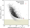 |
Fig. A.1 Correlation of the collisional probabilities p and the impact velocities vimp computed for NEOs larger than 420 m. Our computations were done with (black) and without (gray) gravitational focussing; in both cases p and v is negatively correlated. For reference, the escape speed from Earth, 11.2 km s−1, is also plotted. |
Appendix B Verification by an N-body integration
If we use a direct, N-body integration of known NEOs larger than 420 m, we obtain a very similar result. For this particular computation, we used 3710 orbits from the Astorb catalogue Moskovitz et al. (2022). This number would correspond to the mean geometric albedo of pv = 0.15 (Mainzer et al. 2011). For each orbit, we used 10 clones with different Yarkovsky drifts (Vokrouhlický & Farinella 1999) to account for a possibility of encounters. In this sense, the integration was not deterministic. Eventually, the number of encounters must be divided by 10. The overall time span was 10000 y, the time step 0.009 y, which is sufficient to monitor even the closest encounters with Earth; we recorded all closer than 0.01 au.
Our result is shown in Fig. B.1. We recorded 20990 encounters, 21/10 = 2.1 of them were closer than the 2029 Apophis encounter ( ). The corresponding frequency is thus once per (4760 ± 1040) y, in agreement with Appendix A.
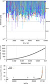 |
Fig. B.1 Top: Close encounter distances vs. time computed for 3710 NEOs larger than ~420 m and their clones (due to the Yarkovsky drift). The total number of bodies was 37100. The number of encounters closer than the 2029 Apophis encounter was 21; the corresponding frequency is approximately once per 4800 y. Middle: Cumulative histogram of distances, N(<r). The dependence is parabolic (as πr2). Bottom: Differential histogram of encounters Nenc per NEO. Only 20% of NEOs underwent encounters closer than 0.01 au in the course of 104 y. Specifically, Apophis clones underwent from 11 to 53 encounters and Apophis-like bodies were responsible for half of all encounters. |
Appendix C Size from occultations
The shape model of Apophis used in this work is based on an extensive set of light curves (Pravec et al. 2014; Ďurech et al. 2026). It is scale-free because visible photometry does not enable us to uniquely determine the albedo. To scale it, we used occultations of stars by Apophis. We computed the sky-plane projections of the model and compared it with the observed occultation timings, projected on the fundamental plane. The size was then optimized so that the distance between the silhouette and the chords was the best in terms of χ2. Details of the method for principal-axis and tumbling rotators were described in Ďurech et al. (2011, 2025).
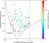 |
Fig. B.2 Apophis-like bodies in the NEO space. Their osculating semimajor axis a and eccentricity e fulfill the conditions Q > 0.983 au, q < 1.016 au, a < 1.523 au, and the number of close encounters with Earth is Nenc(<0.01 au) ≥ 5, computed for 10 clones over 104 y. The colors correspond to the number of encounters. Other NEOs >420 m are also plotted (gray). |
We used four occultations from 2021 (Tab. C.1). Occultation data were obtained from the PDS Small Bodies Node (Herald et al. 2024). Because of the small size of Apophis, the duration of occultations was of the order of 0.1 s. Out of the 12 chords, some have 1-σ errors as large as 0.02 s, but there are four as small as 0.008 s, which constrain the model.
Our result is shown in Fig. C.1. The nominal, volumeequivalent size of Apophis is 417 m, substantially larger than previous nominal values, 340 m and 380 m, respectively (Brozović et al. 2018; Müller et al. 2014). We estimated its uncertainty by a thousand runs with randomly shifted timings (according to the reported errors); the mean value is 420 m and the standard deviation only 14 m.
Non-convexity. Apart from the timing errors, there is a contribution from systematic model errors. In particular, the true shape of Apophis can deviate from our convex-hull shape. We checked several known, non-convex shapes (Eros, Bennu, . . . ) against corresponding convex hulls, and their difference varied from 0.5 up to 5%, in terms of D. If true, the size of Apophis decreases down to 400 m.
For comparison, we scaled the non-convex, radar shape model of Apophis from Brozović et al. (2018) and its volumeequivalent size is 391 m (Fig. C.2). However, it does not fit light curves correctly. The most dramatic deviation from convexity would be binarity. Possibly, it is seen as an ‘eerie darkness’ in some of the Doppler-delay images (Brozović et al. 2018, fig. 2). If true, the size of Apophis decreases further, down to ~380m.
Population estimates. The size of Apophis is linked to our population estimates in Sect. 2.2 and Appendix A. If it is revised from 420 m to ~380m, they must be revised as follows. For the Flora family, which has a shallow slope —1.3, Nmb = 23000 ± 2000, Nneo = 670 ± 150, and the frequency is once per (12000 ± 3100) y. For all NEOs, having the slope -1.9, Nneo = 3980 ± 350, and the corresponding frequency is once per (3900 ± 600) y. None of these revisions would substantially change our conclusions.
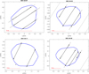 |
Fig. C.1 Convex-hull, light curve shape model of Apophis (this work), scaled to the observed occultations. The resulting volume-equivalent diameter is (420 ± 14) m. This model is preferred. |
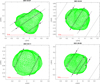 |
Fig. C.2 Non-convex, radar shape model of Apophis (Brozović et al. 2018), scaled to the observed occultations. The resulting volumeequivalent diameter is (391 ± 14) m. This model is substantially different from Fig. C.1, and fits light curves worse than the convex model. |
Appendix D Supplementary figures
For comparison, we show the Juno family in Fig. D.1 and collisions of all NEOs in Fig. D.2.
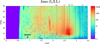 |
Fig. D.1 Same as Fig. 1 but for the Juno family; its distribution would correspond better to L/LL- or L-like NEOs. |
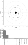 |
Fig. D.2 Same as Fig. 5 but for 3710 NEOs larger than 420 m. In this case, planetary impacts are rare (3.0 ± 0.4%). The time span of simulation (~5 My) corresponded to short-lived NEO orbits. In equilibrium, they are being replenished from the belt. |
The lunar origin suggested for some coorbitals (Jiao et al. 2024) is not feasible for kilometer-sized objects.
All Tables
Source probabilities from five asteroid families (including three dominated by LL compositions) for delivering objects into Apophis-like orbits.
Estimates of populations Nmb(>D), Nneo(>D), and encounter frequencies ∆t for Apophis itself, LL-like NEOs from Flora, and all NEOs.
All Figures
|
Fig. 1 Binned distributions Mj of semimajor axes a and inclinations i of synthetic NEO orbits, originating from individual asteroid families. The colors correspond to the number of test particles in bins, although the quantity Mj(a, i) was eventually normalized. The bin sizes were 0.01 au and 1°, respectively. The Apophis orbit is marked with a black cross. The orbits of other LL-like NEOs from Binzel et al. (2019); Marsset et al. (2022) are marked with gray crosses. Of the three, the highest density for producing Apophis-like objects is from the Flora family. |
| In the text | |
|
Fig. 2 Top: osculating semimajor axis a vs. eccentricity e showing long-term evolution of Apophis-like orbits, after 10Myr. The curves correspond to the boundaries of the NEO space (q < 1.3 au, Q > 0.983 au) and of the adjacent Mars-crossing population. The dotted vertical lines correspond to locations of various mean-motion resonances, including the ν6 secular resonance. The majority of the 100 clones of Apophis remain in the NEO (or Mars-crossing) space; the respective orbit is relatively long-lived. Bottom: number of Apophis clones N vs. time t. The corresponding e-folding timescale is -30 Myr or 50 Myr, respectively, depending on whether or not planetary impacts were used as a criterion for the removal of bodies. |
| In the text | |
|
Fig. 3 Lifetimes of LL-like NEOs originating from the Flora family according to our simulation. The x-axis is simulation time (spanning from 0, i.e., Flora disruption, to 1 Gy, the end of simulation); the y-axis is lifetime. One can see both short-lived orbits (blue) and long-lived orbits (orange); their mix determines the mean lifetime τneo. |
| In the text | |
|
Fig. 4 Top: collisional probabilities of LL-like NEOs originating from the Flora family and their temporal distribution. Individual bodies (out of 1900) are distinguished by shades of gray. The vertical range shows both low and high probabilities. For comparison, the horizontal lines indicate the mean probability p of all NEOs (orange), short-term initial probability p′ of Apophis (cyan), long-term probability p″ of Apophis (green). Bottom: Distribution of all p values (gray) and of the maximum p value (black). |
| In the text | |
|
Fig. 5 Top: collisions of Apophis clones with the Sun, Mercury, Venus, Earth, or Mars. Their positions in the ecliptic frame (x, y) are indicated (crosses), alongside the mean orbital distances of terrestrial planets (dotted circles). Bottom: statistics of collisions. Specifically, (45 ± 2)% of the clones were eliminated due to low perihelion (q < R⊙), while (50 ± 2)% due to planetary impacts. The respective uncertainties (error bars) are Poissonian (∝ √N). |
| In the text | |
|
Fig. 6 Osculating semimajor axis a vs. time t for Apophis clones. When bodies were located within the coorbital region of the Earth (a ∈ (0.995; 1.005) au), e < 0.2), they were plotted in color to distinguish individual bodies, otherwise in gray. |
| In the text | |
|
Fig. 7 Top: observed mean reflectance spectrum of Apophis and Cruithne from the MITHNEOS survey (Binzel et al. 2019; Marsset et al. 2022). Their comparison to taxonomic classes (S, Sq, Q) shows that Apophis is Sq type and Cruithne is Q type. Bottom: same spectra after dereddening (Brunetto et al. 2006); we note the applicability in the visible of this simplified, exp(-CS/λ) model is limited. Their comparison to ordinary chondrite classes (H, L, LL) shows that both asteroids are LL-like. |
| In the text | |
|
Fig. A.1 Correlation of the collisional probabilities p and the impact velocities vimp computed for NEOs larger than 420 m. Our computations were done with (black) and without (gray) gravitational focussing; in both cases p and v is negatively correlated. For reference, the escape speed from Earth, 11.2 km s−1, is also plotted. |
| In the text | |
|
Fig. B.1 Top: Close encounter distances vs. time computed for 3710 NEOs larger than ~420 m and their clones (due to the Yarkovsky drift). The total number of bodies was 37100. The number of encounters closer than the 2029 Apophis encounter was 21; the corresponding frequency is approximately once per 4800 y. Middle: Cumulative histogram of distances, N(<r). The dependence is parabolic (as πr2). Bottom: Differential histogram of encounters Nenc per NEO. Only 20% of NEOs underwent encounters closer than 0.01 au in the course of 104 y. Specifically, Apophis clones underwent from 11 to 53 encounters and Apophis-like bodies were responsible for half of all encounters. |
| In the text | |
|
Fig. B.2 Apophis-like bodies in the NEO space. Their osculating semimajor axis a and eccentricity e fulfill the conditions Q > 0.983 au, q < 1.016 au, a < 1.523 au, and the number of close encounters with Earth is Nenc(<0.01 au) ≥ 5, computed for 10 clones over 104 y. The colors correspond to the number of encounters. Other NEOs >420 m are also plotted (gray). |
| In the text | |
|
Fig. C.1 Convex-hull, light curve shape model of Apophis (this work), scaled to the observed occultations. The resulting volume-equivalent diameter is (420 ± 14) m. This model is preferred. |
| In the text | |
|
Fig. C.2 Non-convex, radar shape model of Apophis (Brozović et al. 2018), scaled to the observed occultations. The resulting volumeequivalent diameter is (391 ± 14) m. This model is substantially different from Fig. C.1, and fits light curves worse than the convex model. |
| In the text | |
|
Fig. D.1 Same as Fig. 1 but for the Juno family; its distribution would correspond better to L/LL- or L-like NEOs. |
| In the text | |
|
Fig. D.2 Same as Fig. 5 but for 3710 NEOs larger than 420 m. In this case, planetary impacts are rare (3.0 ± 0.4%). The time span of simulation (~5 My) corresponded to short-lived NEO orbits. In equilibrium, they are being replenished from the belt. |
| In the text | |
Current usage metrics show cumulative count of Article Views (full-text article views including HTML views, PDF and ePub downloads, according to the available data) and Abstracts Views on Vision4Press platform.
Data correspond to usage on the plateform after 2015. The current usage metrics is available 48-96 hours after online publication and is updated daily on week days.
Initial download of the metrics may take a while.