| Issue |
A&A
Volume 708, April 2026
|
|
|---|---|---|
| Article Number | A282 | |
| Number of page(s) | 11 | |
| Section | The Sun and the Heliosphere | |
| DOI | https://doi.org/10.1051/0004-6361/202558065 | |
| Published online | 14 April 2026 | |
The magnetic sensitivity of the Ca II H and K lines
Institute for Solar Physics, Dept. of Astronomy, Stockholm University, AlbaNova University Centre, 106 91 Stockholm, Sweden
★ Corresponding author: This email address is being protected from spambots. You need JavaScript enabled to view it.
Received:
11
November
2025
Accepted:
4
February
2026
Abstract
Context. The solar chromosphere is a transition layer between the cool, dense photosphere and the hot, rarefied corona. This boundary region plays a key role in regulating energy transport and structuring the magnetic field throughout the solar atmosphere. Understanding its thermodynamic and magnetic properties is essential to model and interpret solar phenomena.
Aims. This study investigates the theoretical properties and diagnostic potential of the polarisation signals in the Ca II H & K lines, with particular emphasis on their capability to probe magnetic fields in the upper chromosphere with the CHROMIS instrument at the Swedish 1-m solar telescope.
Methods. We combine semi-empirical atmospheric models with high-resolution solar observations to model the formation of the Ca II H & K lines using non-local thermodynamic equilibrium radiative transfer calculations. The sensitivity of the lines to the magnetic field is examined through response functions and synthetic inversions, enabling an assessment of their diagnostic performance under realistic chromospheric conditions.
Results. For typical chromospheric field strengths, the linear polarisation of the Ca II H & K lines is less than 1.7%, below the expected detection threshold of CHROMIS. However, their circular polarisation reaches more than 10% in strong-field regions, which is detectable by CHROMIS. Both lines are sensitive to magnetic fields in the upper chromosphere, with the K line forming slightly higher due to its larger opacity, and the H line exhibiting a somewhat stronger Zeeman sensitivity owing to its higher effective Landé factor and longer wavelength. Using the weak-field approximation, the line of sight magnetic field can be reliably inferred around log ξ ≈ −4. These results confirm that the Ca II H & K lines constitute powerful diagnostics for studying the magnetic structure of the upper solar chromosphere.
Key words: Sun: atmosphere / Sun: chromosphere / Sun: magnetic fields / Sun: UV radiation
© The Authors 2026
 Open Access article, published by EDP Sciences, under the terms of the Creative Commons Attribution License (https://creativecommons.org/licenses/by/4.0), which permits unrestricted use, distribution, and reproduction in any medium, provided the original work is properly cited.
This article is published in open access under the Subscribe to Open model. This email address is being protected from spambots. You need JavaScript enabled to view it. to support open access publication.
1. Introduction
Among the many challenges in studies of the solar chromosphere, inferring the magnetic field is one of the most critical and elusive tasks. Magnetic fields play a pivotal role in shaping the energy distribution and dynamic behaviour of the solar atmosphere. Unfortunately, many chromospheric lines suffer from small effective Landé factors, which reduce their sensitivity to the Zeeman effect and complicate magnetic diagnostics. Additionally, few magnetically sensitive lines form in the chromosphere, with the most commonly used line being the central line of the infrared triplet of Ca II at 854.2 nm, which has been the workhorse for chromospheric studies, both in the past (Wiehr & Stellmacher 1991; Pietarila et al. 2007; Kleint 2012; Harvey 2012) and in more recent studies, using high-resolution observations (Kriginsky et al. 2020, 2021; Morosin et al. 2020; Yadav et al. 2021; Vissers et al. 2022). This line has a moderate Landé factor of 1.1, and its formation can be modelled without including complex phenomena such as partial frequency redistribution (PRD) of photons. Additionally, its location in the infrared spectrum provides an advantage as a result of the increased Zeeman splitting at longer wavelengths, enhancing sensitivity to magnetic fields.
The Ca II 854.2 nm line offers several practical benefits for diagnostics. It forms over a relatively broad range of heights, spanning the upper photosphere to the lower chromosphere, and the relatively expanded magnetic field at these heights allows the application of simplified diagnostic techniques such as the weak-field approximation (WFA, Landi Degl’Innocenti & Landolfi 2004).
However, despite its utility, the Ca II 854.2 nm line has limitations. Its sensitivity to magnetic fields peaks in the upper photosphere and lower chromosphere (Quintero Noda et al. 2016) makes it less effective for probing magnetic fields in the middle and upper chromosphere. Therefore, the use of additional spectral lines that form at higher layers is desirable. These lines, while potentially more challenging to model and interpret, can provide the sensitivity needed to diagnose magnetic fields in the upper reaches of the chromosphere.
The Ca II H & K lines at 396.85 nm and 393.37 nm are potentially suitable lines, as they are formed in the middle and upper chromosphere. They are probes of the thermodynamic and kinetic properties of the middle and upper chromosphere (Bjørgen et al. 2018). An alternative set of diagnostics, which has received considerable attention, is the Mg II h and k lines around 280 nm. The Mg II lines have served as the target for magnetic field diagnostics in the chromosphere (Ishikawa et al. 2021; Li et al. 2022, 2024). However, they can only be observed from outside the Earth’s atmosphere, requiring satellite missions or rocket experiments. In contrast, the Ca II H and K lines can be observed from the ground, making them more suitable for routine spectropolarimetric campaigns.
However, the use of Ca II H and K lines in spectropolarimetry remains under-explored (Martinez Pillet et al. 1990). This limitation is due to a combination of factors. First, the photon flux in the blue part of the spectrum is lower compared to the red part, reducing the S/N in observations. Second, the effective Landé factors of these lines (1.169 for the Ca II K line and 1.33 for the Ca II H line) suggest that their sensitivity to magnetic fields may be modest. However, in active regions, the line profiles vary strongly, which corresponds to steep intensity gradients (dI/dλ, e.g. Leenaarts et al. 2018). As a result, the circular polarisation signal can still reach more than 10% of the intensity, despite the modest Landé factor (Martinez Pillet et al. 1990).
The polarisation of the Ca II H & K lines is subject to the effects of phenomena that are neglected in most inversion studies, such as atomic polarisation and J-state interference (Belluzzi & Trujillo Bueno 2011; Juanikorena Berasategi et al. 2025). Some properties of the linear polarisation seen in these lines can only be explained by accounting for these phenomena. An example is the zero-level crossing of the linear polarisation fraction between the core of both lines described by Stenflo (1980), which can be reproduced when quantum interferences are accounted for (Belluzzi & Trujillo Bueno 2011).
Recent and forthcoming advances in instrumentation are likely to renew interest in the spectropolarimetric signal of the Ca II H and K lines. Spectropolarimeters capable of observing the blue part of the visible spectrum have already been developed. For example, the Sunrise UV Spectropolarimeter and Imager (SUSI, Feller et al. 2020) instrument on board the SUNRISE III balloon experiment (Korpi-Lagg et al. 2025) and the Visible Spectro-Polarimeter (ViSP, de Wijn et al. 2022) at the Daniel K. Inouye Solar Telescope (DKIST, Rimmele et al. 2020) are tailored for such studies. The CHROMospheric Imaging Spectrometer (CHROMIS; Scharmer 2017) at the Swedish 1-meter solar telescope (SST, Scharmer et al. 2003) was upgraded in the spring of 2025 to allow for full-Stokes spectropolarimetry in Ca II H & K. It is undergoing calibration and testing as of the summer of 2025.
The purpose of this study is to investigate the magnetic sensitivity of the Ca II H and K lines, along with their potential use for magnetic field diagnostics. This goal is primarily motivated by the advantages and disadvantages of CHROMIS. It is a dual Fabry-Pérot-based imaging spectropolarimeter for the 390–500 nm range, and can operate simultaneously with the CRISP2 instrument (Scharmer et al. 2026). The latter is a new instrument for the 500–900 nm range that replaced the old CRISP instrument (Scharmer et al. 2008) in the summer of 2025. Both instruments can obtain images with a diffraction-limited spatial resolution. One scientific goal of these instruments is to observe multiple spectral lines together and use these observations as input to multi-line multi-spatial-resolution inversions (de la Cruz Rodríguez 2019) in order to produce full 3D models of the thermodynamic and magnetic properties of the solar photosphere and chromosphere. Adding spectropolarimetric capabilities to CHROMIS helps to constrain the magnetic field in the middle and upper chromosphere.
Because of the low photon flux in the Ca II H & K lines and the need to scan wavelengths in the line consecutively, we do not expect to achieve an S/N larger than ∼200 without sacrificing too much in temporal cadence. We thus want to investigate whether we can expect to observe this linear polarisation at all because linear polarisation signals tend to be weaker than circular polarisation. Given this limitation, we also want to investigate whether it is required to include atomic polarisation and J-state interference. Adding those processes adds orders of magnitude to the time required for inversions (on the order of 103 hour per pixel, Li et al. 2022) compared to inversions that only include the Zeeman effect, which take less than one hour per pixel.
Finally, given the large field of view (FOV) of CHROMIS (80 × 80 arcsec corresponding to ∼2200 × 2200 pixels), even a Zeeman-effect-only inversion of a single line scan would take on the order of 106 CPU hours. Therefore, we also investigate the accuracy of the WFA in these lines, as this would give a quick way to get a rough idea of the magnetic field that can be run on a small computer.
To do this, we start with investigating the expected polarisation signal in a semi-empirical model atmosphere for atomic polarisation, J-state interference, and the Zeeman effect. We will show that for the expected S/N of CHROMIS observations, we can only expect to see circular polarisation signals caused by the Zeeman-effect. Then we create a 3D empirical model atmosphere from which we compute synthetic Ca II H & K spectra. We invert these spectra with the weak-field approximation to investigate the accuracy of the derived magnetic field compared to the ground truth.
2. Methods
2.1. Synthesis code
One of our goals is to determine the importance of applying the correct theoretical formalism when solving the line formation problem for the Ca II H & K lines. For this purpose, we employ the HanleRT code (del Pino Alemán et al. 2016), which can solve the line formation problem accounting for the joint action of the Zeeman effect, J-state interference, and atomic polarisation mechanisms for arbitrary magnetic fields. HanleRT incorporates the multi-term formalism of Casini et al. (2014), including the effects of possible coherences that are neglected when using a multilevel formalism, while also accounting for the effects of PRD. We use this code to generate spectral profiles under the multilevel and multiterm approximations, to determine when the multilevel approach is sufficiently accurate in reproducing the polarimetric properties of these lines.
2.2. Observations
For our study, we would ideally use real spectropolarimetric observations in the Ca II H & K lines obtained with instruments such as CHROMIS. However, these data are not available yet and we needed to consider an alternative. We decided to use atmospheric models obtained from spectropolarimetric inversions applied to observations. We used this approach instead of performing the synthesis of data from numerical simulations because simulation spectra have been shown to be considerably different from observed ones (Bjørgen et al. 2018).
We used observations obtained on 17 October 2023 with the CRISP imaging spectropolarimeter (Scharmer et al. 2008, CRISP) at the SST starting at 10:26:10 UT. The observations were performed in a 3 × 3 mosaic mode, with an overlap of 30%, providing an overview of the active region NOAA 13465 as it neared the disc centre. Spectropolarimetric observations of the Ca II 854.2 nm line were obtained at 15 wavelength positions, sampling the interval [−6.75, 6.75] ×10−2 nm around the line core. Raw data were reduced with the SSTRED processing pipeline (de la Cruz Rodríguez et al. 2015; Löfdahl et al. 2021), including image restoration using the Multi-Object Multi-Frame Blind Deconvolution (MOMFBD; Löfdahl 2002; Van Noort et al. 2005) method.
This particular observation is an ideal target for the current study, as it spans a large FOV near disc centre, including pixels located in the active region sunspot, the surrounding plage areas, and large quiet-Sun regions (see Fig. 1).
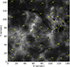 |
Fig. 1. Image of active region NOAA 13465 in the line core of the Ca II 854.2 nm line. The marked pixels are the locations of 45 representative line profiles that sample the variety of line profiles present in the observations as determined by k-means clustering (see Sect. 2.4). |
2.3. Inversion code
We perform spectropolarimetric inversions on the observations of the Ca II 854.2 nm line to obtain an empirical 3D atmospheric model. We also used inversions of synthetic spectra of the Ca II H & K lines computed from this model to determine how accurate the magnetic fields inverted from their spectra can be.
To perform the inversions we used the STockholm inversion Code (STiC, de la Cruz Rodríguez et al. 2016, 2019), an inversion tool that incorporates a modified version of the Rybicki and Hummer code (RH, Uitenbroek 2001) as its forward solver under the assumption of a 1D plane-parallel atmosphere. Within STiC, the radiative transfer equation is solved using cubic Bézier solvers (de la Cruz Rodríguez & Piskunov 2013). The inversion process also relies on an equation of state extracted from the Spectroscopy Made Easy code (SME, Piskunov & Valenti 2017), and includes the effects of PRD following Leenaarts et al. (2012).
2.4. The inversion strategy
We applied the k-means clustering method to the observations described in Sect. 2.2, obtaining 45 clusters. We then used STiC to invert one profile from each cluster (identified in Fig. 1) to obtain atmospheric models that together form a representative sample of the variety of atmospheres that one might encounter when observing the chromosphere.
For each chosen profile, the FAL-C atmosphere was used as an initial guess, with an ad-hoc vertical velocity stratification added. Each pixel was inverted, assuming either a constant velocity or one varying with depth. The inversions were carried out at 50 equidistant depth points within the column mass range log ξ ∈ [ − 6.5, 1.0]. The column mass, ξ, represents the integrated mass per unit area above a given height, defined as
 (1)
(1)
where ρ is the mass density, ds is the differential path length along the vertical direction. In centimetre-gram-seconds (cgs) units, ξ is expressed in g cm−2.
Multiple inversion cycles were performed, increasing the number of nodes after each cycle. The inverted physical parameters were the temperature T, the vertical velocity v, the microturbulent velocity vturb, the parallel and perpendicular magnetic field components (BLoS and BPoS, respectively) and the azimuth angle χ. The number of nodes for each parameter and cycle is given in Table 1.
Node distribution for each of the inversion cycles.
The first two cycles were devoted to the determination of the stratification of temperature and vertical velocity, while the magnetic field was kept undetermined. The third and fourth cycles were used only for the magnetic inversion, using as an initial guess the value obtained through the use of the weak-field approximation.
For each pixel, we chose the atmospheric model that yielded the smallest value of the χ2 function, defined as
 (2)
(2)
where wk, i is the weight associated with the noise level of the Stokes parameter k at the wavelength index i, s is the number of wavelength points, Iobs is the observed Stokes vector, and Imod is the Stokes vector produced by the forward engine of the inversion code given the input stratification of the inverted physical parameters.
We then inverted the full FOV consisting of 10 890 000 pixels. To make the task computationally feasible, we adopted the following scheme:
-
The pixels in the FOV were randomly divided into 40 groups.
-
For the first group, each pixel was initialised using the atmospheric model corresponding to the k-means cluster to which it belonged.
-
These pixels were inverted with STiC using three inversion cycles, employing node configurations equivalent to cycles 2, 4, and 5 of Table 1.
-
A neural network was then trained to reproduce the inverted atmospheres from this first group, using the observed Stokes profiles as input. The network architecture was adapted from Kriginsky & Oliver (2025), with additional parallel branches to estimate the magnetic field stratification.
-
For each of the remaining pixel groups:
-
the neural network (continually updated after each group) was used to predict an initial atmospheric model for every pixel in the group;
-
these pixels were then inverted with STiC using the same three-cycle scheme as in Step 3;
-
the neural network was retrained by including the newly inverted pixels, progressively improving its predictions.
-
-
This process was repeated until all 40 groups had been inverted.
This hybrid inversion–prediction approach, with the neural network acting as an intermediate step, reduced the total inversion time by a factor of at least three.
3. Results
3.1. Semi-empirical atmosphere
We compared the multilevel Zeeman approximation (MZ) with the multiterm formalism (MT) to assess the errors introduced by the simplified MZ approach in reproducing the spectra of the Ca II H & K lines. The calculations were carried out using the semi-empirical FAL-C model (Avrett 1985; Fontenla et al. 1993), with a constant ad hoc magnetic field. For the MZ approach, we employed a five-level plus continuum Ca II atom, whereas for the MT approach a three-term Ca II atom was considered (Del Pino Aleman, private communication). In both cases, PRD was included in the Ca II H and K lines, while the infrared triplet lines were treated under the assumption of complete redistribution (CRD).
3.1.1. Non-magnetic case
We first considered the formation of fractional linear polarisation profiles in the absence of magnetic fields. For this test, we fixed the azimuth angle so that U = 0. Figure 2 compares the results of the MZ and MT approaches for different values of the heliocentric angle μ. The MT approach reproduces the expected zero-level crossing between the cores of the two lines and the small lobes around the core of the Ca II H line, already reproduced in previous studies (Belluzzi & Trujillo Bueno 2011; Juanikorena Berasategi et al. 2025) for μ < 1. Because the atmosphere is assumed to be plane-parallel, no linear polarisation is produced for μ = 1. As expected, the MZ approach cannot reproduce the effects of quantum interferences, as those are neglected, and predicts incorrect linear polarisation in the wings of the lines. However, both approaches yield nearly identical results for the core of the Ca II K line.
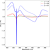 |
Fig. 2. Comparison of linear polarisation of the Ca II H and K lines computed with the multiterm (MT, solid curves) and multilevel (ML, dashed curves) formalisms for different values of the heliocentric angle μ for the case of zero magnetic field. The colours represent the different values of μ as given in the legend. For μ = 1 no scattering polarisation is produced and both curves are identically zero. |
3.1.2. Magnetic case
To evaluate the effects of the presence of a uniform, non-zero magnetic field on the fractional polarisation under both the MZ and MT formalisms, we performed a spectral synthesis for different values of the total magnetic field strength (B). The magnetic field inclination with respect to the vertical direction was kept fixed at 45°. Figure 3 shows the fractional total linear polarisation ( ) under both formalisms for different values of the total magnetic field strength and heliocentric angle.
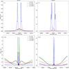 |
Fig. 3. Fractional linear polarisation of the Ca II H and K lines under the multilevel and multiterm formalisms. As in Fig. 2, continuous curves represent the results of the MT formalism, while the results of the MZ formalism are shown in dashed curves. The different colours represent different values of B, which is shown inside the panels. The top panels show the results viewed at disc centre (μ = 1), while the bottom panels show the results for μ = 0.6. The panels on the left show the results for the Ca II K line, while the panels on the right side show the results for the Ca II H line. |
We start by looking at the result for μ = 1. Because the model atmosphere is plane-parallel, there is no scattering polarisation, and the non-zero TLP is caused by the Zeeman effect. The signals are weak, and even at B = 707 G (i.e the horizontal component of the field is 500 G), the maximum TLP/Icont is only 0.4%.
Towards the limb (bottom panels), the magnetic field has a depolarising effect, with the value of TLP/Icont decreasing in both the line core and the line wings with an increasing magnetic field. The maximum TLP/Icont (for zero field) is above 1.5%, decreasing to 0.8% for a field of 42 G, and we speculate that TLP signals originating from weak-field regions might just be visible with CHROMIS.
The agreement between both formalisms is good around the core of the Ca II K line. The fact that the Ca II H line is intrinsically unpolarisable means that the MZ modelling will be unable to reproduce the correct line profiles for magnetic fields that do not give rise to significant Zeeman-induced linear polarisation.
Based on the results of Fig. 3 we do not expect to see any TLP (i.e. Stokes Q and U) at disc center outside of regions with very strong horizontal fields (such as penumbras). That is because for an instrument like CHROMIS, whose maximum expected S/N level is 200 for the intensity, fractional linear polarisation levels below 0.5 % are expected to be below the detection threshold. Therefore, if the observational target is a weak-field region, observed Stokes Q and U will likely be an effect of calibration errors in the observations.
3.1.3. Circular polarisation
We synthesised the Stokes V profiles for different values of BLoS for μ = 1 using MZ and MT formalisms. The results are presented in Fig. 4. The outputs from both formalisms are virtually identical. As the circular polarisation in the Ca II H and K lines is predominantly dominated by the Zeeman-induced polarisation, the results for other heliocentric angles bear great resemblance to the result presented for μ = 1, so they are not shown here.
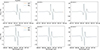 |
Fig. 4. Fractional circular polarisation of the Ca II H and K lines under the multilevel and multiterm formalisms for different values of B when observed at disc centre. Again, as in Fig. 2, solid curves represent the results of the MT formalism, while the results of the MZ formalism are shown in dashed curves. The panels on the top show the Ca II K line profiles, and the panels on the bottom show the Ca II H line profiles. |
The circular polarisation signals of the Ca II H and K lines are orders of magnitude stronger than the corresponding linear polarisation signals (upper panel of Fig. 3). This large amplitude underscores the potential to use the Stokes V signal for chromospheric magnetic field diagnostics.
However, the spectral profiles shown in Fig. 3 and Fig. 4 were computed at a much higher spectral resolution than is typically achievable in observations with instruments such as CHROMIS. Additionally, these profiles do not incorporate the effects of noise, which would further complicate the analysis and reduce the usability of the weaker linear polarisation signals. We investigate these effects in the following sections.
3.2. Synthetic profiles
We now turn our attention from the FAL-C atmosphere to the 3D model atmosphere that we constructed from the Ca II 854.2 nm observations (see Sect. 2.4).
We used the inverted atmospheres of the 45 representative pixels of each k-mean cluster to compute synthetic spectra using STiC of the Ca II H and K lines. This step allowed us to evaluate the polarisation signals that are expected from different solar structures.
As in the semi-empirical atmosphere discussed in Sect.3.1, the fractional linear polarisation (Q/Icont and U/Icont) in all cases was well below 1%. Therefore, we focus on the circular polarisation (V), whose results are shown for three representative clusters in the second row of Fig. 5, and for all clusters in Fig. A.1.
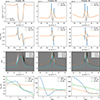 |
Fig. 5. Line profiles, response functions, and magnetic fields in three representative atmosphere models. Top row: Intensity of the Ca II H line before (blue) and after (orange) being convolved with a spectral PSF of 130 mÅ. Second row: Circular polarisation of the Ca II H line before (blue) and after (orange) being convolved with a spectral PSF of 130 mÅ. Third row: Image of the response functions of Stokes V in the Ca II H line to variations of BLoS, as function of wavelength expressed as Doppler shift and column mass ξ. The three dashed curves correspond to the location on the log ξ vs Δλ space of the maxima of the response functions for the Ca II H (blue), K (orange), and 854.2 nm (cyan) lines. Bottom row: Stratification of BLoS obtained from inverting the synthesized Ca II H and K spectra compared to the input atmospheric model. Vertical lines on the bottom row represent estimations of the uncertainty of the BLoS at chosen depth points. |
The synthetic Stokes V profiles display a wide range of behaviours, reflecting the diversity of solar structures sampled by the observations. The maximum circular polarisation fraction spans from about 0.2% in clusters located in regions of weak line-of-sight magnetic field to values as large as 20% in magnetic field concentrations. Most clusters lie between these extremes. As expected, pixels with lower polarisation fractions correspond to areas far from photospheric magnetic concentrations, often in fibrillar regions where the magnetic field is largely horizontal. Conversely, the largest polarisation fractions are found in clusters associated with strong magnetic field concentrations, where both the field strength and BLoS are high.
3.2.1. Response functions
To investigate where in the atmosphere the Ca II H and K lines are sensitive to magnetic fields, we computed numerical response functions of Stokes V to BLoS with STiC for the 45 representative pixels. The third row of Fig. 5 shows the results for three clusters described earlier, while the response functions for all 45 clusters are provided in Fig. A.2. The response functions of the Ca II K line are nearly identical to those of the H line and are omitted here for clarity.
Most response functions are not antisymmetric with respect to the line core. In fact, at the same wavelength one can often find both positive and negative values at different depths. This behaviour is consistent with the presence of vertical gradients in the source function (Uitenbroek 2006). An inspection of the source function as a function of height confirmed that such gradients are indeed present in all the relevant profiles.
In the wings of the lines, the response is mainly to magnetic fields low in the atmosphere (around log ξ = −1). Closer to the line cores, the response is much stronger, and Stokes V becomes sensitive to magnetic fields in the upper chromosphere, with a maximum of the response function above log ξ = −4. For comparison with the Ca II 854.2 nm line, the dashed curves in the third row of Fig. 5 show the height of the maximum of the absolute value of the response function as a function of wavelength for all three lines. The results clearly indicate that the Ca II H and K lines (blue and orange curves) probe magnetic fields at greater heights than their infrared counterpart (cyan curve).
Due to its larger opacity, the Ca II K line is sensitive to slightly higher atmospheric layers than the Ca II H line, although the two largely overlap. Assuming hydrostatic equilibrium, we find that at line centre the difference in height of the response-peak locations between the two lines varies between about 90 and 130 km. Consequently, spectropolarimetric observations of both lines can provide not only redundancy but also complementary information, helping to better constrain magnetic field values in the upper chromosphere, provided that the observations achieve sufficient S/N. Comparatively, the difference in height of the response-peak locations between the Ca II K and Ca II 854.2 nm line is around 400 km.
3.2.2. Ca II H & K inversions
Building on the results of the response functions, we next tested whether BLoS can be constrained through inversions of the Ca II H and K spectropolarimetric profiles. For this purpose, we used STiC to invert the synthetic spectra of the three representative pixels shown in Fig. 5.
Inversions were performed in two cycles: first to constrain the temperature, line-of-sight velocity, and microturbulent velocity, and then a second cycle with one, two, or three nodes in BLoS. The inversion with the lowest value of χ was chosen as the best fit. To evaluate the impact of instrumental spectral PSF, we performed inversions both with and without convolving the synthetic spectra with the CHROMIS PSF, which has a full width at half-maximum of 0.13 Å. The bottom row of Fig. 5 shows, for each pixel, the stratification recovered in BLoS compared to the original atmosphere. For those pixels, the cycle with two nodes in BLoS yielded the lowest value of χ. We used the numerical response functions to estimate the uncertainty of the obtained BLoS at three depth points using the method described in del Toro Iniesta (2003).
The results vary depending on the strength of the polarisation signal. For the pixel with weak circular polarisation (left column), inversion without PSF recovers the overall behaviour of BLoS, but the retrieval degrades when PSF is included. For the intermediate case (middle column), where the chromospheric magnetic field is stronger, both inversions reproduce the magnetic field at higher layers reasonably well, although the lower-layer field is not constrained, consistent with the limited sensitivity of the H and K lines to deep layers. Finally, for the pixel with the strongest chromospheric magnetic field and polarisation signal (right column), the inversion with PSF convolution actually outperforms the one without, yielding a better match to the input stratification.
3.2.3. Weak field approximation
We showed in Sect. 3.2.2 that full non-LTE inversions can retrieve a good estimate of the magnetic field in the chromosphere. However, such inversions take ∼1 h of CPU time per pixel, and it would be desirable to obtain an estimate of the field that is quicker to compute. This is particularly important for time series of CHROMIS observations, which contain ∼5 × 10⁶ spatial pixels per line scan.
Therefore, we applied the WFA to the synthetic Ca II H profiles. Based on the response function analysis in Sect. 3.2.1, we restricted the calculation to a 0.04 nm window around the Ca II H line core, where sensitivity to upper-chromospheric magnetic fields is strongest. Weak-field calculations were performed with and without convolving the profiles with the CHROMIS spectral PSF (FWHM = 0.13 Å) using a typical spectral sampling of 0.065 nm. To simulate the conditions of real observations, we also repeated the calculations adding a noise level of 5 × 10⁻³. We used the spatially-regularised WFA method of de la Cruz Rodríguez & Leenaarts (2024) to perform the magnetic field inference.
The results are presented in Fig. 6. We used the structural similarity index (SSIM, Wang & Bovik 2009), which quantifies the similarity between two maps based on their intensity patterns and spatial structure through local mean, variance, and cross-covariance. Our analysis shows that the weak-field estimate of BLoS matches the input atmosphere at log ξ ≈ −4 best, consistent with the sensitivity derived from the response functions. The corresponding BLoS map is shown in panel (a) of Fig. 6. Comparison of panels (b) and (c) indicates that convolution with the spectral PSF does not introduce significant differences. This is further supported by the logarithmic density plots in panels (e) and (f), which show nearly identical scatter relative to the input atmosphere. However, adding noise, as shown in panels (d) and (g), degrades the quality of the inferred BLoS. Specifically, the density plot in panel (g) exhibits a substantial increase in scatter compared to the noiseless case. A summary of the density plots is provided in Table 2, which lists various percentile values. For BLoS inference without PSF convolution and without added noise, the 50% percentile value is 6 G. This indicates that for 50% of the pixels, the difference between the inferred BLoS using the weak-field approximation and the input BLoS at log ξ = −4 is less than 6 G. Table 2 confirms that PSF convolution has minimal impact, with the 50% percentile unchanged and the 70% percentile increasing by less than 5 G. In contrast, added noise significantly affects the results: the 50% percentile is nearly three times larger than the noiseless case, and the 70% percentile is almost twice as large.
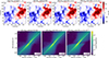 |
Fig. 6. Top row: Line-of-sight magnetic field (BLoS) at log ξ = −4 from the input model (a), compared with the weak-field estimates obtained from the original synthetic spectra (b), and from the same spectra after convolution with the CHROMIS spectral PSF with (c), and without noise (d). Bottom row: Logarithmic density plots comparing the input BLoS with the weak-field results, for the case without the convolution with the PSF (e), and with the convolution with the PSF for the noiseless case (f) and the case with added noise (g). Dashed lines in the bottom row mark the identity line. |
4. Conclusions
In this work, we explored the diagnostic potential of the Ca II H and K lines to probe magnetic fields in the solar chromosphere. To this end, we combined forward modelling and inversions based on both semi-empirical atmospheric models and atmospheres retrieved from high-resolution observations.
A first step was to assess the validity of the MZ approximation compared with the more complete MT formalism. We confirmed that the MZ approximation is inadequate for reproducing the formation of linear polarisation in these lines, consistent with earlier studies (Stenflo 1980; Belluzzi & Trujillo Bueno 2011; Juanikorena Berasategi et al. 2025). However, we also showed that circular polarisation can be reliably modelled under the MZ formalism, meaning that widely used inversion codes such as STiC (de la Cruz Rodríguez et al. 2019) can be safely applied to this observable.
From both semi-empirical and inverted model atmospheres, we synthesised spectropolarimetric profiles and examined their polarisation properties. The linear polarisation amplitudes are weak (below 1.7% in our tests), making them hard to detect with an instrument like CHROMIS. The circular polarisation, in contrast, shows a wide range of amplitudes, from fractions of a percent in quiet-Sun conditions to more than 10% in strong magnetic concentrations, even if the observations have a spectral resolution of 30 000.
The response functions to BLoS showed that the wings of the Ca II H and K lines are sensitive to magnetic fields in the lower chromosphere (around log ξ = −1), while their cores respond to magnetic fields higher in the chromosphere, peaks above log ξ = −4. Compared to the commonly used Ca II 854.2 nm line, the Ca II H and K lines probe higher atmospheric layers.
Although the peak response depths of the Ca II H and K lines largely overlap, they are not identical: assuming hydrostatic equilibrium, the location of the peak response at line core differs by approximately 90 to 130 km. This offset reflects intrinsic differences between the two transitions: the K line, having the larger oscillator strength, and thus opacity, tends to form slightly higher in the atmosphere, whereas the H line has a larger effective Landé factor and a marginally larger wavelength. Consequently, the Zeeman splitting, which scales as ΔλB ∝ geffλ2B, is somewhat larger for the H line, providing a modest enhancement in magnetic sensitivity per unit of field strength. In practice, the K line exhibits stronger line depression but lower photon flux, while the H line offers slightly larger S/N under comparable observing conditions (see Fig. A.1).
We further tested the feasibility of constraining BLoS through inversions of synthetic Ca II H and K line profiles. For representative pixels, the inversions were able to recover the magnetic field in the upper chromosphere, even when the profiles were degraded by the CHROMIS spectral PSF. To extend the analysis to the full field of view, we inverted the Ca II 854.2 nm observations with STiC. The resulting atmospheric models were used to synthesise Ca II H and K line profiles, to which we applied the weak-field approximation. Using the structure similarity index, we found that the weak-field estimate BLoS best matches the input atmosphere around log ξ = −4, consistent with the response function analysis. Even at spectral resolution, the number of spectral samples and noise level that we expect to obtain with CHROMIS, BLoS are retrieved well.
Together, these results establish that the Ca II H and K lines offer sensitivity to line-of-sight magnetic fields in the upper chromosphere, at heights inaccessible with the popular chromospheric diagnostics obtained from the Ca II 854.2 nm line (e.g. Kuridze et al. 2019; Morosin et al. 2020), while also being observable from the ground, in contrast to the Mg II h and k lines (Ishikawa et al. 2021).
The large amplitude of the circular polarisation signal indicates that the CHROMIS instrument will be able to use the Ca II H & K lines for inference of the line-of-sight magnetic field. However, the linear polarisation signals are too weak to reliably obtain estimates of the magnetic field in the plane of sky.
Acknowledgments
The authors of this paper gratefully acknowledge funding by the European Union through the European Research Council (ERC) under the Horizon Europe program (MAGHEAT, grant agreement 101088184), and the Swedish Research Council (registration number 2022-03535 and 2021-05613), and Swedish National Space Agency (2021-00116). The Swedish 1-m Solar Telescope is operated on the island of La Palma by the Institute for Solar Physics of Stockholm University in the Spanish Observatorio del Roque de los Muchachos of the Instituto de Astrofísica de Canarias. The Institute for Solar Physics is supported by a grant for research infrastructures of national importance from the Swedish Research Council (registration number 2021-00169). The computations were enabled by resources provided by the National Academic Infrastructure for Supercomputing in Sweden (NAISS), partially funded by the Swedish Research Council through grant agreement no. 2022-06725. The authors acknowledge the National Academic Infrastructure for Supercomputing in Sweden (NAISS), partially funded by the Swedish Research Council through grant agreement no. 2022-06725, for awarding this project access to the LUMI supercomputer, owned by the EuroHPC Joint Undertaking and hosted by CSC (Finland) and the LUMI consortium.
References
- Avrett, E. H. 1985, in Chromospheric Diagnostics and Modelling, ed. B. W. Lites, 67 [Google Scholar]
- Belluzzi, L., & Trujillo Bueno, J. 2011, ApJ, 743, 3 [NASA ADS] [CrossRef] [Google Scholar]
- Bjørgen, J. P., Sukhorukov, A. V., Leenaarts, J., et al. 2018, A&A, 611, A62 [Google Scholar]
- Casini, R., Landi Degl’Innocenti, M., Manso Sainz, R., Landi Degl’Innocenti, E., & Landolfi, M. 2014, ApJ, 791, 94 [NASA ADS] [CrossRef] [Google Scholar]
- de la Cruz Rodríguez, J. 2019, A&A, 631, A153 [NASA ADS] [CrossRef] [EDP Sciences] [Google Scholar]
- de la Cruz Rodríguez, J., & Leenaarts, J. 2024, A&A, 685, A85 [NASA ADS] [CrossRef] [EDP Sciences] [Google Scholar]
- de la Cruz Rodríguez, J., & Piskunov, N. 2013, ApJ, 764, 33 [Google Scholar]
- de la Cruz Rodríguez, J., Löfdahl, M. G., Sütterlin, P., & Hillberg, T. 2015, & Rouppe van der Voort. L., A&A, 573, A40 [Google Scholar]
- de la Cruz Rodríguez, J., Leenaarts, J., & Asensio Ramos, A. 2016, ApJ, 830, L30 [Google Scholar]
- de la Cruz Rodríguez, J., Leenaarts, J., Danilovic, S., & Uitenbroek, H. 2019, A&A, 623, A74 [Google Scholar]
- de Wijn, A. G., Casini, R., Carlile, A., et al. 2022, Sol. Phys., 297, 22 [NASA ADS] [CrossRef] [Google Scholar]
- del Pino Alemán, T., Casini, R., & Manso Sainz, R. 2016, ApJ, 830, L24 [Google Scholar]
- del Toro Iniesta, J. C. 2003, Introduction to Spectropolarimetry (Cambridge, UK: Cambridge University Press) [Google Scholar]
- Feller, A., Gandorfer, A., Iglesias, F. A., et al. 2020, in Ground-based and Airborne Instrumentation for Astronomy VIII, eds. C. J. Evans, J. J. Bryant, & K. Motohara, SPIE Conf. Ser., 11447, 11447AK [NASA ADS] [Google Scholar]
- Fontenla, J. M., Avrett, E. H., & Loeser, R. 1993, ApJ, 406, 319 [Google Scholar]
- Harvey, J. W. 2012, Sol. Phys., 280, 69 [NASA ADS] [CrossRef] [Google Scholar]
- Ishikawa, R., Trujillo Bueno, J., del Pino Alemán, T., et al. 2021, Sci. Adv., 7, eabe8406 [NASA ADS] [CrossRef] [Google Scholar]
- Juanikorena Berasategi, I., Alsina Ballester, E., del Pino Alemán, T., & Trujillo Bueno, J., 2025, A&A, 704, A173 [NASA ADS] [CrossRef] [EDP Sciences] [Google Scholar]
- Kleint, L. 2012, ApJ, 748, 138 [Google Scholar]
- Korpi-Lagg, A., Gandorfer, A., Solanki, S. K., et al. 2025, Sol. Phys., 300, 75 [Google Scholar]
- Kriginsky, M., & Oliver, R. 2025, ApJ, 981, 121 [Google Scholar]
- Kriginsky, M., Oliver, R., Freij, N., et al. 2020, A&A, 642, A61 [EDP Sciences] [Google Scholar]
- Kriginsky, M., Oliver, R., Antolin, P., Kuridze, D., & Freij, N. 2021, A&A, 650, A71 [NASA ADS] [CrossRef] [EDP Sciences] [Google Scholar]
- Kuridze, D., Mathioudakis, M., Morgan, H., et al. 2019, ApJ, 874, 126 [Google Scholar]
- Landi Degl’Innocenti, E., & Landolfi, M. 2004, Polarization in Spectral Lines,, 307 (Dordrecht: Kluwer Academic Publishers) [Google Scholar]
- Leenaarts, J., Pereira, T., & Uitenbroek, H. 2012, A&A, 543, A109 [NASA ADS] [CrossRef] [EDP Sciences] [Google Scholar]
- Leenaarts, J., de la Cruz Rodríguez, J., Danilovic, S., Scharmer, G., & Carlsson, M. 2018, A&A, 612, A28 [NASA ADS] [CrossRef] [EDP Sciences] [Google Scholar]
- Li, H., del Pino Alemán, T., Trujillo Bueno, J., & Casini, R. 2022, ApJ, 933, 145 [NASA ADS] [CrossRef] [Google Scholar]
- Li, H., del Pino Alemán, T., & Trujillo Bueno, J. 2024, ApJ, 975, 110 [Google Scholar]
- Löfdahl, M. G. 2002, in Image Reconstruction from Incomplete Data, eds. P. J. Bones, M. A. Fiddy, & R. P. Millane, SPIE Conf. Ser., 4792, 146 [CrossRef] [Google Scholar]
- Löfdahl, M. G., Hillberg, T., de la Cruz Rodríguez, J., et al. 2021, A&A, 653, A68 [Google Scholar]
- Martinez Pillet, V., Garcia Lopez, R. J., del Toro Iniesta, J. C., et al. 1990, ApJ, 361, L81 [NASA ADS] [CrossRef] [Google Scholar]
- Morosin, R., de la Cruz Rodríguez, J., Vissers, G. J. M., & Yadav, R. 2020, A&A, 642, A210 [NASA ADS] [CrossRef] [EDP Sciences] [Google Scholar]
- Pietarila, A., Socas-Navarro, H., & Bogdan, T. 2007, ApJ, 663, 1386 [Google Scholar]
- Piskunov, N., & Valenti, J. A. 2017, A&A, 597, A16 [NASA ADS] [CrossRef] [EDP Sciences] [Google Scholar]
- Quintero Noda, C., Shimizu, T., de la Cruz Rodríguez, J., et al. 2016, MNRAS, 459, 3363 [Google Scholar]
- Rimmele, T. R., Warner, M., Keil, S. L., et al. 2020, Sol. Phys., 295, 172 [Google Scholar]
- Scharmer, G. 2017, in SOLARNET IV: The Physics of the Sun from the Interior to the Outer Atmosphere, 85 [Google Scholar]
- Scharmer, G. B., Bjelksjo, K., Korhonen, T. K., Lindberg, B., & Petterson, B. 2003, The 1-m Swedish Solar Telescope, 4853 [Google Scholar]
- Scharmer, G. B., de la Cruz Rodríguez, J., Leenaarts, J., Lindberg, B., et al. 2026, A&A, 705, A55 [NASA ADS] [CrossRef] [EDP Sciences] [Google Scholar]
- Scharmer, G. B., Narayan, G., Hillberg, T., et al. 2008, ApJ, 689, L69 [Google Scholar]
- Stenflo, J. O. 1980, A&A, 84, 68 [NASA ADS] [Google Scholar]
- Uitenbroek, H. 2001, ApJ, 557, 389 [Google Scholar]
- Uitenbroek, H. 2006, in Solar MHD Theory and Observations: A High Spatial Resolution Perspective, eds. J. Leibacher, R. F. Stein, & H. Uitenbroek, ASP Conf. Ser., 354, 313 [NASA ADS] [Google Scholar]
- Van Noort, M., Der Voort, L. R. V., & Löfdahl, M. G. 2005, Solar Physics, 228, 191 [Google Scholar]
- Vissers, G. J. M., Danilovic, S., Zhu, X., et al. 2022, A&A, 662, A88 [NASA ADS] [CrossRef] [EDP Sciences] [Google Scholar]
- Wang, Z., & Bovik, A. C. 2009, IEEE Signal Process. Mag., 26, 98 [Google Scholar]
- Wiehr, E., & Stellmacher, G. 1991, A&A, 247, 379 [NASA ADS] [Google Scholar]
- Yadav, R., Díaz Baso, C. J., de la Cruz Rodríguez, J., Calvo, F., & Morosin, R. 2021, A&A, 649, A106 [NASA ADS] [CrossRef] [EDP Sciences] [Google Scholar]
Appendix A: K-means groups inversions and response functions
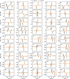 |
Fig. A.1. Expanded version of the top row of Fig. 5, including all the identified clusters with their respective Ca II H & K line profiles. The cluster numbers are shown in black inside each panel. |
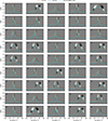 |
Fig. A.2. Expanded version of the third row of Fig. 5, including all the identified clusters. The cluster numbers are shown in black inside each panel. |
All Tables
All Figures
|
Fig. 1. Image of active region NOAA 13465 in the line core of the Ca II 854.2 nm line. The marked pixels are the locations of 45 representative line profiles that sample the variety of line profiles present in the observations as determined by k-means clustering (see Sect. 2.4). |
| In the text | |
|
Fig. 2. Comparison of linear polarisation of the Ca II H and K lines computed with the multiterm (MT, solid curves) and multilevel (ML, dashed curves) formalisms for different values of the heliocentric angle μ for the case of zero magnetic field. The colours represent the different values of μ as given in the legend. For μ = 1 no scattering polarisation is produced and both curves are identically zero. |
| In the text | |
|
Fig. 3. Fractional linear polarisation of the Ca II H and K lines under the multilevel and multiterm formalisms. As in Fig. 2, continuous curves represent the results of the MT formalism, while the results of the MZ formalism are shown in dashed curves. The different colours represent different values of B, which is shown inside the panels. The top panels show the results viewed at disc centre (μ = 1), while the bottom panels show the results for μ = 0.6. The panels on the left show the results for the Ca II K line, while the panels on the right side show the results for the Ca II H line. |
| In the text | |
|
Fig. 4. Fractional circular polarisation of the Ca II H and K lines under the multilevel and multiterm formalisms for different values of B when observed at disc centre. Again, as in Fig. 2, solid curves represent the results of the MT formalism, while the results of the MZ formalism are shown in dashed curves. The panels on the top show the Ca II K line profiles, and the panels on the bottom show the Ca II H line profiles. |
| In the text | |
|
Fig. 5. Line profiles, response functions, and magnetic fields in three representative atmosphere models. Top row: Intensity of the Ca II H line before (blue) and after (orange) being convolved with a spectral PSF of 130 mÅ. Second row: Circular polarisation of the Ca II H line before (blue) and after (orange) being convolved with a spectral PSF of 130 mÅ. Third row: Image of the response functions of Stokes V in the Ca II H line to variations of BLoS, as function of wavelength expressed as Doppler shift and column mass ξ. The three dashed curves correspond to the location on the log ξ vs Δλ space of the maxima of the response functions for the Ca II H (blue), K (orange), and 854.2 nm (cyan) lines. Bottom row: Stratification of BLoS obtained from inverting the synthesized Ca II H and K spectra compared to the input atmospheric model. Vertical lines on the bottom row represent estimations of the uncertainty of the BLoS at chosen depth points. |
| In the text | |
|
Fig. 6. Top row: Line-of-sight magnetic field (BLoS) at log ξ = −4 from the input model (a), compared with the weak-field estimates obtained from the original synthetic spectra (b), and from the same spectra after convolution with the CHROMIS spectral PSF with (c), and without noise (d). Bottom row: Logarithmic density plots comparing the input BLoS with the weak-field results, for the case without the convolution with the PSF (e), and with the convolution with the PSF for the noiseless case (f) and the case with added noise (g). Dashed lines in the bottom row mark the identity line. |
| In the text | |
|
Fig. A.1. Expanded version of the top row of Fig. 5, including all the identified clusters with their respective Ca II H & K line profiles. The cluster numbers are shown in black inside each panel. |
| In the text | |
|
Fig. A.2. Expanded version of the third row of Fig. 5, including all the identified clusters. The cluster numbers are shown in black inside each panel. |
| In the text | |
Current usage metrics show cumulative count of Article Views (full-text article views including HTML views, PDF and ePub downloads, according to the available data) and Abstracts Views on Vision4Press platform.
Data correspond to usage on the plateform after 2015. The current usage metrics is available 48-96 hours after online publication and is updated daily on week days.
Initial download of the metrics may take a while.