| Issue |
A&A
Volume 708, April 2026
|
|
|---|---|---|
| Article Number | A237 | |
| Number of page(s) | 12 | |
| Section | Atomic, molecular, and nuclear data | |
| DOI | https://doi.org/10.1051/0004-6361/202558232 | |
| Published online | 08 April 2026 | |
Simulation of proton radiolysis of H2O and O2 ices with the Nautilus code
1
School of Astronomy & Space Science, Nanjing University,
163 Xianlin Avenue,
Nanjing
210023,
China
2
Laboratoire d’Astrophysique de Bordeaux, Univ. Bordeaux, CNRS, B18N, allée Geoffroy Saint-Hilaire,
33615
Pessac,
France
3
Institut des Sciences Moléculaires (ISM), CNRS, Univ. Bordeaux,
351 cours de la Libération,
33400
Talence,
France
4
Laboratoire des deux infinis Irène Joliot Curie (IJClab), CNRS-IN2P3, Université Paris-Saclay,
91405
Orsay,
France
5
Institut des Sciences Moléculaires d’Orsay (ISMO), UMR8214, CNRS, Université Paris-Saclay,
Bât 520, Rue André Rivière,
91405
Orsay,
France
6
Key Laboratory of Modern Astronomy and Astrophysics, Nanjing University, Ministry of Education,
Nanjing
210023,
China
★ Corresponding authors: This email address is being protected from spambots. You need JavaScript enabled to view it.
; This email address is being protected from spambots. You need JavaScript enabled to view it.
Received:
24
November
2025
Accepted:
23
February
2026
Abstract
Context. The radiolysis effect of cosmic rays (CRs) plays an important role in the chemistry of molecular clouds. Cosmic rays can dissociate molecules on dust grains, producing reactive suprathermal species and radicals, which facilitate the formation of large molecules.
Aims. In this study, we attempt to reproduce laboratory experimental results on the radiolysis of pure H2O and O2 ice using the Nautilus astrochemical code, and evaluate the effects of varying several uncertain physical and chemical parameters.
Methods. We added radiolysis reactions, quenching reactions of suprathermal species, and reactions between suprathermal and thermal species to the Nautilus code. By adjusting the parameters in the code, we investigated the sensitivity of the simulation results for H2O ice to the removal of reaction-diffusion competition, the removal of non-diffusive chemistry, and the desorption energies of suprathermal species.
Results. We find that the Nautilus model, with a few adjustments to the chemistry, reproduces the steady-state [H2O2]/[H2O] and [O3]/[O2]0 abundance ratios in the H2O and O2 radiolysis experiments at any CR flux explored. However, these adjustments do not fully reproduce the fluence required to reach the steady state. The model also tends to overestimate the destruction of H2O measured in H2O radiolysis experiments. We show that reducing the G-values of H2O radiolysis, which implies an increase in the efficiency of immediate local reformation of water molecules after impact by ions, leads to simulated H2O destruction rates that are closer to experimental results. The effect of reaction-diffusion competition on the simulation results for H2O ice is significant only at ζ ≲ 10−14 s−1. Non-diffusive chemistry affects the simulation results at 16 K but not at 77 K, while the results are sensitive to the desorption energies of suprathermal H, O, O3 and OH at 77 K.
Conclusions. Our results show that the steady-state [H2O2]/[H2O] and [O3]/[O2]0 in radiolysis experiments can be reproduced by fine-tuning the chemical model, but still call for further constraints on the intermediate pathways in the radiolysis processes, especially the ion chemistry in the ice bulk, as well as activation barriers and branching ratios of the reactions in the network.
Key words: astrochemistry / ISM: abundances / cosmic rays / ISM: molecules
© The Authors 2026
 Open Access article, published by EDP Sciences, under the terms of the Creative Commons Attribution License (https://creativecommons.org/licenses/by/4.0), which permits unrestricted use, distribution, and reproduction in any medium, provided the original work is properly cited.
This article is published in open access under the Subscribe to Open model. This email address is being protected from spambots. You need JavaScript enabled to view it. to support open access publication.
1 Introduction
Cosmic rays (CRs) are energetic charged particles (~106−1018 eV) that consist of protons, heavy ions, and electrons. They permeate our Galaxy and strongly influence the physics and chemistry of the interstellar medium (ISM; e.g., Dalgarno 2006; Indriolo & McCall 2013; Gaches & Viti 2026). The heating effect of CRs plays an important role in the thermal balance of the ISM (Goldsmith & Langer 1978). Low-energy CRs act as the primary source of ionization in dense molecular clouds (MCs) shielded from UV radiation (Padovani et al. 2009; Chabot 2016). Cosmic rays ionize molecular hydrogen through the reaction
![Mathematical equation: $\[\mathrm{H}_2 \xrightarrow{\mathrm{CR}} \mathrm{H}_2^{+}+\mathrm{e}^{-},\]$](/articles/aa/full_html/2026/04/aa58232-25/aa58232-25-eq1.png) (1)
(1)
whose rate coefficient is defined as the CR ionization rate per H2 molecule. This quantity is widely used to characterize the degree of CR ionization in MCs and is typically on the order of 10−17−10−16 s−1 (e.g., Caselli et al. 1998; Indriolo & McCall 2012; Neufeld & Wolfire 2017; Bovino et al. 2020; Neufeld et al. 2024; Obolentseva et al. 2024; Bialy et al. 2026; Neufeld et al. 2026; Indriolo et al. 2026). The ![Mathematical equation: $\[\mathrm{H}_{2}^{+}\]$](/articles/aa/full_html/2026/04/aa58232-25/aa58232-25-eq2.png) ion then reacts with H2 to form
ion then reacts with H2 to form ![Mathematical equation: $\[\mathrm{H}_{3}^{+}\]$](/articles/aa/full_html/2026/04/aa58232-25/aa58232-25-eq3.png) , which initiates the formation of polyatomic molecules in the gas phase in MCs. Cosmic rays can also ionize He to form He+, which in turn dissociates CO in MCs to form C and C+, thereby affecting our understanding of the molecular inventory in galaxies (Bisbas et al. 2015, 2017). Moreover, CRs are believed to be a source of UV radiation within dense MCs (Prasad & Tarafdar 1983).
, which initiates the formation of polyatomic molecules in the gas phase in MCs. Cosmic rays can also ionize He to form He+, which in turn dissociates CO in MCs to form C and C+, thereby affecting our understanding of the molecular inventory in galaxies (Bisbas et al. 2015, 2017). Moreover, CRs are believed to be a source of UV radiation within dense MCs (Prasad & Tarafdar 1983).
In addition to gas-phase ionization, CRs release molecular species from the dust mantle back to the gas phase via global heating of grains (Léger et al. 1985; Hasegawa & Herbst 1993), impulsive spot heating of grains (Ivlev et al. 2015), photodesorption by secondary UV photons induced by CRs (Öberg et al. 2007; Ruaud et al. 2016), and sputtering (Dartois et al. 2018; Wakelam et al. 2021). These non-thermal desorption processes have been proposed as the origin of complex organic molecules (COMs) observed in cold cores (e.g., Bacmann et al. 2012). Radiolysis is another important CR process that can facilitate the formation of COMs in cold cores (e.g., Pilling et al. 2010; de Barros et al. 2011). When CRs collide with dust grains, primary CR particles and secondary electrons dissociate molecules in ice mantles to form radicals and suprathermal species, which are highly reactive and enhance the production of COMs (Shingledecker et al. 2018). This effect has been extensively studied in laboratory experiments. For example, HCOOH and CH3OH are produced after irradiation of a mixture of H2O and CO2 ice by 0.8 MeV protons (Hudson & Moore 1999). Similar experiments were conducted with energetic electrons (e.g., Bennett et al. 2005; Zheng et al. 2006) and with heavy ions as CR analogs (e.g., Palumbo et al. 2000; Baratta et al. 2002; Seperuelo Duarte et al. 2010; Boduch et al. 2012). These experiments strongly suggest that radiolysis alters the chemical composition of ice and triggers the formation of large molecules.
Radiolysis needs to be considered in complex astrochemical models to make them more realistic. Before doing so, the model needs to be benchmarked against experiments. Shingledecker & Herbst (2018) propose a method to introduce ice radiolysis into chemical models based on rate equations. The authors explored the results of radiolysis in a dark MC using a complex chemical model. By incorporating radiolysis into the MONACO code (the MONte cArlo COde; Vasyunin & Herbst 2013; Vasyunin et al. 2017), Shingledecker et al. (2019, hereafter SVHC19) successfully reproduced the experimental results of H2O and O2 ice irradiated by protons (Baragiola et al. 1999; Gomis et al. 2004a). Using the same method, the simulation of Paulive et al. (2021) suggests that the abundances of some COMs, such as HCOOCH3 and CH2OHCHO, in dark MCs are enhanced by radiolysis. A similar method was also used to simulate the experiment of O2 ice exposed to ionizing UV radiation (Mullikin et al. 2021). In contrast, Pilling et al. (2022, 2023) simulated the radiolysis experiments of H2O and CO2 ices and obtained the reaction rates by fitting the experimental results.
In this paper, we expand the work of SVHC19 by simulating proton-irradiated H2O and O2 ice using another chemical model, Nautilus. In sophisticated chemical models, many parameters are tunable, often with scarce constraints from experiments or theoretical calculations. We explore how selected parameters affect the simulated chemistry in irradiated H2O and O2 ice. The paper is organized as follows. In Section 2, we describe how we modify the chemical model and construct the reaction network. Section 3 presents the simulation results for H2O and O2 and several test models, which we discuss in Section 4. We summarize our findings in Section 5.
2 Model and network
2.1 Chemical model
The simulation is based on the Nautilus code, which is a three-phase rate-equation chemical model (Ruaud et al. 2016). The experiments we considered were conducted in thick ices with little to no interactions with the gas. To simulate the chemical processes in the experiments, we considered only bulk species and removed all gas-phase reactions, surface-bulk swapping, adsorption and desorption, and photodissociation by CR-induced UV photons. Following SVHC19, we included the following radiolysis processes in the code:
![Mathematical equation: $\[\mathrm{A} \rightsquigarrow \mathrm{~A}^{+}+\mathrm{e}^{-} \rightarrow \mathrm{A}^* \rightarrow \mathrm{~B}^*+\mathrm{C}^*\]$](/articles/aa/full_html/2026/04/aa58232-25/aa58232-25-eq4.png) (R1)
(R1)
![Mathematical equation: $\[\mathrm{A} \rightsquigarrow \mathrm{~A}^* \rightarrow \mathrm{~B}+\mathrm{C},\]$](/articles/aa/full_html/2026/04/aa58232-25/aa58232-25-eq5.png) (R2)
(R2)
![Mathematical equation: $\[\mathrm{A} \rightsquigarrow \mathrm{~A}^*,\]$](/articles/aa/full_html/2026/04/aa58232-25/aa58232-25-eq6.png) (R3)
(R3)
where the curly arrow indicates the dissociation reaction resulting from collision with CR protons or secondary electrons, and asterisks mark suprathermal species. In process R1, the target species A is ionized by the incident particle, but soon recombines to form suprathermal A*, which is then dissociated into suprathermal B* and C*. In processes R2 and R3, species A is directly excited to the suprathermal state, and in process R2 the suprathermal A* dissociates into B* and C*. We approximate the reaction rate coefficients of these processes to first order as (Shingledecker & Herbst 2018)
![Mathematical equation: $\[k=S_{\mathrm{e}}\left(\frac{G}{100 \mathrm{eV}}\right) \phi\left(\frac{\zeta}{10^{-17} \mathrm{~s}^{-1}}\right),\]$](/articles/aa/full_html/2026/04/aa58232-25/aa58232-25-eq7.png) (2)
(2)
where Se is the electronic stopping power of species A at a given energy of the incident particle, the G-value is the number of molecules destroyed per 100 eV transferred from the incident particles to the irradiated ice (Dewhurst et al. 1952), ϕ = 8.6 particles cm−2 s−1 is the integrated interstellar CR flux (Spitzer & Tomasko 1968), and ζ is the CR ionization rate. We adopted all simulated radiolysis processes and their G values from Shingledecker et al. (2018) and SVHC19 and list them in Table 1. Unlike SVHC19, which used the same H2O stopping power, Se, of Baragiola et al. (1999) for all species, we calculated Se values for each molecular species using the SRIM code (Stopping and Range of Ions in Matter; Ziegler et al. 2010). Table 1 also lists the Se values for two different energies, corresponding to the energies of impacting particles used in the reference experiments.
Suprathermal species are quenched by the bulk mantle to thermal species or react diffusively and nondiffusively with another thermal icy species. The quenching reaction can be written as
![Mathematical equation: $\[\mathrm{A}^* \longrightarrow \mathrm{~A},\]$](/articles/aa/full_html/2026/04/aa58232-25/aa58232-25-eq8.png) (R4)
(R4)
where A is an arbitrary species. Its rate coefficient (in s−1) is the characteristic vibrational frequency of species A,
![Mathematical equation: $\[\nu_{\mathrm{A}}=\sqrt{\frac{2 N_{\text {site}} E_{\mathrm{D}}^{\mathrm{A}}}{\pi^2 m_{\mathrm{A}}}},\]$](/articles/aa/full_html/2026/04/aa58232-25/aa58232-25-eq9.png) (3)
(3)
where ![Mathematical equation: $\[E_{\mathrm{D}}^{\mathrm{A}}\]$](/articles/aa/full_html/2026/04/aa58232-25/aa58232-25-eq10.png) (in K) and mA (in g) are the desorption energy and mass of species A, and Nsite is the number of sites per grain.
(in K) and mA (in g) are the desorption energy and mass of species A, and Nsite is the number of sites per grain.
Reactions between suprathermal and thermal species (denoted as A* and B, respectively) can proceed through both diffusive and nondiffusive mechanisms. The rate coefficient for diffusive reactions was introduced in Ruaud et al. (2016):
![Mathematical equation: $\[k_{\mathrm{diff}}=f_{\mathrm{br}} \kappa_{\mathrm{AB}}\left[\nu_{\mathrm{A}} \exp \left(-\frac{E_{\mathrm{diff}}^{\mathrm{A}}}{T_{\mathrm{ice}}}\right)+\nu_{\mathrm{B}} \exp \left(-\frac{E_{\mathrm{diff}}^{\mathrm{B}}}{T_{\mathrm{ice}}}\right)\right] \frac{1}{N_{\mathrm{site}} n_{\mathrm{dust}}},\]$](/articles/aa/full_html/2026/04/aa58232-25/aa58232-25-eq11.png) (4)
(4)
where fbr is the branching ratio, κAB is the probability of the reaction occurring, ![Mathematical equation: $\[E_{\text {diff}}^{\mathrm{A}}\]$](/articles/aa/full_html/2026/04/aa58232-25/aa58232-25-eq12.png) and
and ![Mathematical equation: $\[E_{\text {diff}}^{\mathrm{B}}\]$](/articles/aa/full_html/2026/04/aa58232-25/aa58232-25-eq13.png) (in K) are the diffusion barriers of A and B, and ndust is the gas-phase concentration of dust particles (in cm−3). We set κAB = 1 for exothermic, barrierless reactions (Hasegawa et al. 1992), but calculated κAB as the result of the competition between reaction and diffusion for exothermic reactions with activation barriers (Chang et al. 2007; Garrod & Pauly 2011; Ruaud et al. 2016). This modification of the surface rate coefficients mimics the fact that two species on the same site are more likely to remain together than to diffuse apart, increasing the probability of a reaction despite the barrier. The SVHC19 model did not include this competition for the ice bulk. We included this competition in our simulation; its effect is presented in Section 3.6. The SVHC19 model uses the MONACO code, as described in Vasyunin et al. (2017) and Vasyunin & Herbst (2013). Vasyunin & Herbst (2013) justify this because most, if not all, activation barriers for surface processes are based on gas-phase experiments, where this process does not occur. Another important difference between Nautilus and MONACO is that MONACO includes modified rate equations that account for stochastic effects in surface chemistry, as proposed by Garrod (2008). In models without reaction-diffusion competition, we computed κAB following Hasegawa et al. (1992), i.e., assuming quantum-mechanical tunneling probabilities. We explore the influence of reaction-diffusion competition in Section 3.6.
(in K) are the diffusion barriers of A and B, and ndust is the gas-phase concentration of dust particles (in cm−3). We set κAB = 1 for exothermic, barrierless reactions (Hasegawa et al. 1992), but calculated κAB as the result of the competition between reaction and diffusion for exothermic reactions with activation barriers (Chang et al. 2007; Garrod & Pauly 2011; Ruaud et al. 2016). This modification of the surface rate coefficients mimics the fact that two species on the same site are more likely to remain together than to diffuse apart, increasing the probability of a reaction despite the barrier. The SVHC19 model did not include this competition for the ice bulk. We included this competition in our simulation; its effect is presented in Section 3.6. The SVHC19 model uses the MONACO code, as described in Vasyunin et al. (2017) and Vasyunin & Herbst (2013). Vasyunin & Herbst (2013) justify this because most, if not all, activation barriers for surface processes are based on gas-phase experiments, where this process does not occur. Another important difference between Nautilus and MONACO is that MONACO includes modified rate equations that account for stochastic effects in surface chemistry, as proposed by Garrod (2008). In models without reaction-diffusion competition, we computed κAB following Hasegawa et al. (1992), i.e., assuming quantum-mechanical tunneling probabilities. We explore the influence of reaction-diffusion competition in Section 3.6.
Another important process is nondiffusive chemistry. This process mimics the fact that when species are abundant, their probability of being formed nearby by photoprocesses or radiolysis is so high that they react without having to diffuse (Jin & Garrod 2020). The SVHC19 model shows that including this process is crucial. We therefore included the formalism from SVHC19 with a slight modification:
![Mathematical equation: $\[k_{\text {non-diff }}=f_{\text {br }}\left(\frac{\nu_{\mathrm{A}}+\nu_{\mathrm{B}}}{\max \left(N_{\text {bulk }}, N_{\text {site }}\right)}\right) \exp \left(-\frac{E_{\text {act }}^{\mathrm{AB}}}{T_{\text {ice }}}\right),\]$](/articles/aa/full_html/2026/04/aa58232-25/aa58232-25-eq22.png) (5)
(5)
where Nbulk is the total number of bulk species in the simulated ice, rather than the number of sites on a single grain as in SVHC19. This modification accounts for the dilution of species in the mantle in a more realistic way and decreases the efficiency of nondiffusive chemistry. The quantity ![Mathematical equation: $\[E_{\text {act}}^{\mathrm{AB}}\]$](/articles/aa/full_html/2026/04/aa58232-25/aa58232-25-eq23.png) denotes the activation barrier of the reaction. The formula corresponds to Equation (4) assuming immediate diffusion, that is,
denotes the activation barrier of the reaction. The formula corresponds to Equation (4) assuming immediate diffusion, that is, ![Mathematical equation: $\[\exp (-E_{\text {diff}}^{\mathrm{A}} / T_{\text {ice}})=1\]$](/articles/aa/full_html/2026/04/aa58232-25/aa58232-25-eq24.png) . In Nautilus, we also included the formalism from Jin & Garrod (2020), which is entirely different. However, with the reduced network used here, the code did not converge because the destruction rates of minor species with nondiffusive chemistry were much higher than their production rate. We conclude that the formalism of Jin & Garrod (2020) cannot be applied in this case.
. In Nautilus, we also included the formalism from Jin & Garrod (2020), which is entirely different. However, with the reduced network used here, the code did not converge because the destruction rates of minor species with nondiffusive chemistry were much higher than their production rate. We conclude that the formalism of Jin & Garrod (2020) cannot be applied in this case.
The SVHC19 model mostly tested the effect of species diffusion efficiency in ice by comparing three models: the first includes nondiffusive chemistry, the second includes only thermal hopping of the species, and the third allows H, H2, and O to diffuse through tunneling effects. In our simulations, we allowed all species to diffuse through tunneling, but their efficiency depended on their mass (Wakelam et al. 2024). We explore the effect of nondiffusive chemistry in Sections 3.7.
We adopted the desorption energies (ED) of the simulated species from SVHC19, except for H and H2 and list them in Table 2 for quantitative comparison with the results. For H and H2, the desorption energies are 650 K and 440 K, respectively (Wakelam et al. 2017). For the other species, we assumed diffusion barriers of 0.7ED (as in SVHC19). We assumed identical desorption energies and diffusion barriers for suprathermal species and their corresponding thermal species. We investigate the influence of changing the desorption energies in Section 3.8.
Throughout the simulation, we maintained a gas density of nH = 109 cm−3 and a gas-to-dust mass ratio of 100. Variations in gas density do not affect the simulation results. We set the CR ionization rate to 1.3 × 10⁻⁷ s−1, corresponding to an ion flux of ~1.1 × 10¹¹ particles cm−2 s−1. This is significantly higher than the CR ionization rates in the ISM (Caselli et al. 1998; Indriolo & McCall 2012), but is consistent with the flux used in SVHC19 simulations and matches the typical ion flux used in experiments (e.g., Gomis et al. 2004b,a). We discuss the effect of CR ionization rates on the simulation results in Section 3.4.
Radiolysis processes considered in the simulations, including branching ratios, G-values, process types, and calculated stopping powers (10−14 eV cm2 molecule−1) for each species.
Desorption energies of the simulated species.
2.2 Reaction network
Table 3 shows the reaction network, which is based on Table 4 of SVHC19 for H2O2, with some modifications. It contains 38 reactions for nine bulk species. As stated above, we ignore gas-phase and surface reactions, as well as any exchanges between them and the bulk. Some reactions lack activation barriers in the references. Following SVHC19, we assumed unknown barriers of 10 000 K, except for radical-radical reactions, for which we assumed barriers of 0. For each thermal reaction A + B → product in Table 3, we included both the diffusive and nondiffusive pathways for reactions involving thermal radicals and atomic O. The original references for activation energies and branching ratios are provided in SVHC19. Some values have been updated and we provide the new references in the Table. Reactions involving thermal atomic H do not include the nondiffusive pathways by default because H can diffuse rapidly in the ice. We also included the diffusive and nondiffusive pathways for reactions involving suprathermal species:
![Mathematical equation: $\[\mathrm{A}^*+\mathrm{B} \longrightarrow \text { product, }\]$](/articles/aa/full_html/2026/04/aa58232-25/aa58232-25-eq25.png) (R5)
(R5)
![Mathematical equation: $\[\mathrm{A}+\mathrm{B}^* \longrightarrow \text { product.}\]$](/articles/aa/full_html/2026/04/aa58232-25/aa58232-25-eq26.png) (R6)
(R6)
We assumed zero activation barriers for reactions involving suprathermal species.
In addition to the reactions in Table 3, we included the reactions of O, O2, and O3 in Table 7 of Shingledecker et al. (2017); we list this part of the network in Table 4. We treated the electronically excited species in Shingledecker et al. (2017) as suprathermal species that can react with thermal species without a barrier. We include both diffusive and non-diffusive pathways for reactions in Table 4.
2.3 Conversion among ion fluence, energy dose, and simulation time
We express the abundances of the simulated species in the chemical model as a function of simulation time (t). Experimental abundances are given as a function of ion fluence or energy dose, with
![Mathematical equation: $\[\text { dose }=\text { fluence } \text { \times } S_{\mathrm{e}} \text {. }\]$](/articles/aa/full_html/2026/04/aa58232-25/aa58232-25-eq27.png) (6)
(6)
We define the ion fluence as the total number of impinging proton per area, in units of protons cm−2, and it can be directly monitored in experiments; we define the energy dose as the total energy absorbed by the target species, in units of eV molecule−1. As a first-order approximation, the dose is the governing parameter that determines the result of the radiolysis process. We calculated the relation between the experimental dose and the simulated time as follows. We first adopted an approximated equation for the CR spectral density (Shen et al. 2004):
![Mathematical equation: $\[j_n=\frac{9.42 \times 10^4 E^{0.3}}{\left(E+E_0\right)^3} \text { particles } \mathrm{cm}^{-2} \mathrm{~s}^{-1} \mathrm{~sr}^{-1}(\mathrm{MeV} / \mathrm{nucl})^{-1},\]$](/articles/aa/full_html/2026/04/aa58232-25/aa58232-25-eq28.png) (7)
(7)
where E is the CR energy and E0 is a form parameter between 0–940 MeV, which determines the spectra of low-energy CRs. To determine the value of E0, we fit the normalization (Padovani et al. 2009)
![Mathematical equation: $\[1.7 \times 4 \pi \sum_Z f_Z \int_{0.1 ~\mathrm{MeV}}^{10 ~\mathrm{GeV}} j_n(E, Z) \sigma(E, Z) ~d E=10^{-17} \mathrm{~s}^{-1},\]$](/articles/aa/full_html/2026/04/aa58232-25/aa58232-25-eq42.png) (8)
(8)
where Z is the nuclear charge of the CR species, fZ is the abundance of the CR species, fZ is the abundance of the CR species Z, jn(E, Z) is the CR spectral density of a CR species Z with an energy of E, σ(E, Z) = Z2σ(E, Z = 1) is the H2 ionization cross section of a CR species Z with an energy of E adopted from Rudd et al. (1983), and 10−17 s−1 on the right hand side of the equation is the characteristic CR ionization rate used in Equation (9). The coefficient 1.7 accounts for the effect of secondary electrons during ionization. We considered H, He, C, N, O, Mg, Si, and Fe in the CR constituents and adopted the abundances in Kalvāns (2018), and obtained E0 = 637 MeV. We then calculated the relation between dose and time using
![Mathematical equation: $\[\text { dose }=4 \pi t\left(\frac{\zeta}{10^{-17} \mathrm{~s}^{-1}}\right) \sum_Z f_Z \int_{0.1 ~\mathrm{MeV}}^{10 ~\mathrm{GeV}} j_n(E, Z) S_{\mathrm{e}}(E, Z) ~d E,\]$](/articles/aa/full_html/2026/04/aa58232-25/aa58232-25-eq43.png) (9)
(9)
where ζ is the CR ionization rate per H2 adopted in the simulation. After substituting the CR spectral densities of different CR constituents, jn(E, Z), obtained from Equations (7) and (8), as well as the stopping powers of the CR constituents, Se (E, Z), injected into H2O and O2 ice calculated with SRIM, we find
![Mathematical equation: $\[\frac{\text { dose }}{\mathrm{eV} / \text { atom }}=\left(\frac{t}{\mathrm{yr}}\right)\left(\frac{\zeta}{10^{-17} \mathrm{~s}^{-1}}\right) \times\left\{\begin{array}{l}1.82 \times 10^{-8} \text { for } \mathrm{H}_2 \mathrm{O} \text { ice, } \\4.14 \times 10^{-8} \text { for } \mathrm{O}_2 \text { ice, }\end{array}\right.\]$](/articles/aa/full_html/2026/04/aa58232-25/aa58232-25-eq44.png) (10)
(10)
where the dose is given per atom in the target icy molecular species, H2O and O2. In the following sections, we present the simulated results as functions of ion fluence.
Reaction network considered here, based on Table 7 of Shingledecker et al. (2017).
3 Simulation results
3.1 Experimental data of proton-irradiated pure H2O and O2 ice
3.1.1 Pure H2O ice
Using the chemical model and reaction network introduced in Section 2, we simulated the chemistry of pure thick H2O ice irradiated by 200 keV protons at 16 K and 77 K. As in SVHC19, we compared our model results with the experiments conducted by Gomis et al. (2004a), who obtained a maximum [H2O2]/[H2O] abundance ratio of 1.2% at 16 K and 0.4% at 77 K. If we assume that the column density of H2O remains constant throughout the experiment, the experimental [H2O2]/[H2O] as a function of ion fluence can be fitted by
![Mathematical equation: $\[\frac{\left[\mathrm{H}_2 \mathrm{O}_2\right]}{\left[\mathrm{H}_2 \mathrm{O}\right]}=\left(\frac{\left[\mathrm{H}_2 \mathrm{O}_2\right]}{\left[\mathrm{H}_2 \mathrm{O}\right]}\right)_{\max }\left(1-\mathrm{e}^{-\sigma_{\mathrm{d}} F}\right),\]$](/articles/aa/full_html/2026/04/aa58232-25/aa58232-25-eq45.png) (11)
(11)
where F is the fluence and σd is the destruction cross-section of H2O2. The results of Gomis et al. (2004a) can be fitted with σd = 9 × 10⁻¹⁵ cm2 and 1.6 × 10⁻¹⁴ cm2 at 16 K and 77 K, respectively. From the column density evolution of water ice upon irradiation presented in Fig. 1 of Gomis et al. (2004a), we estimate that ≲8% of the initial H2O is destroyed by 200 keV He+ ion at 16 K at large fluence, providing an upper limit to the total number of species that can be produced. We obtain the expected destruction of H2O in a proton-irradiated H2O experiment by scaling this result from the He+ experiment using the ratio of the stopping powers of protons (1.93 × 10⁻¹⁴ eV cm molecule−1) and He+ (4.98 × 10⁻¹⁴ eV cm2 molecule−1) in H2O ice. We therefore evaluate that ≲3.1% of the initial H2O is destroyed after irradiation with 200 keV protons at the same fluences at 16 K.
Loeffler et al. (2006) concluded a similar experiment with pure H2O ice exposed to 100 keV protons at 20 K and 80 K and concluded that the maximum [H2O2]/[H2O] was 0.75% at 20 K and 0.14% at 80 K. Although the temperature difference may contribute to the resulting maximum [H2O2]/[H2O], we roughly assume that the typical uncertainty in the experimental results is a factor of three.
Gomis et al. (2004a) and Loeffler et al. (2006) report only the [H2O2]/[H2O] value. However, experiments with pure H2O ice exposed to other ionizing radiation also suggest products of proton-irradiated H2O ice, which we focus on. When exposed to UV photons composed of Lyman-α (121.6 nm) and molecular H2 emission bands (130–165 nm), H2O ice can produce O2 and H2O2 with [O2]/[H2O2] ~ 0.7 at 20 K (Bulak et al. 2022). When H2O ice is irradiated by 5 keV electrons, H2, O2, and H2O2 form with [H2] : [H2O2] : [O2] ≈ 160 : 13 : 1 at 12 K (Zheng et al. 2006). Although the exact amounts of the products differ in proton-irradiated H2O ice, these experiments show that significant amounts of H2 and O2 form together with H2O2.
3.1.2 Pure O2 ice
Pure O2 ice is the simplest system for proton irradiation experiments and simulations, with only three species O, O2 and O3 to consider. Ennis et al. (2011) conducted an experiment exposing O2 ice to 5 keV protons at 12 K. They obtained a steady state O3 column density of 1.5 × 1016 cm−2, with an initial O2 column density of 3.8 × 1018 cm−3. In this section, we compare our simulation results with this experimental value, [O3]/[O2]0 = 0.395% ([O2]0 refers to the initial abundance of O2 ice) with an uncertainty of a factor of three. Although Ennis et al. (2011) did not fit the fluence-dependent evolution of O3 ice, they reported that the O3 column density reached steady state after an irradiation time of 2.5 × 10⁴ s, which corresponds to a fluence of ~7.6 × 10¹⁵ ions cm−2.
Baragiola et al. (1999) conducted a similar experiment, irradiating pure O2 ice with 100 keV protons at 5 K. Simulations (SVHC19) reproduce the O3 density. However, Baragiola et al. (1999) did not report the density of O2 in their experiment. The SVHC19 model adopted the initial O2 density from Hörl & Kohlbeck (1982). Since this value was not directly obtained from the experiment of Baragiola et al. (1999), it can introduce additional uncertainty into the analysis. Therefore, we chose the Ennis et al. (2011) experiment as our reference for greater consistency.
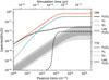 |
Fig. 1 Simulation results of abundance ratios [H2O2]/[H2O] (black lines), [H2]/[H2O] (orange lines), and [O2]/[H2O] (blue lines) with our model (model A) at 16 K (solid lines) and 77 K (dashed lines). The shaded gray and line-filled regions show the experimental results of [H2O2]/[H2O] by Gomis et al. (2004a) at 16 and 77 K, respectively, with an assumed uncertainty of a factor of three. |
3.2 Best-fit model results
3.2.1 Pure H2O ice
Figure 1. shows the simulation results for proton-irradiated pure H2O ice at 16 K and 77 K obtained with our model (hereafter model A; see the description in Section 2 for details). The abundance ratios [H2O2]/[H2O], [H2]/[H2O], and [O2]/[H2O] increase monotonically with ion fluence when the fluence is ≲ 3 × 10¹³ ions cm−2 and then reach steady states. The steady-state [H2O2]/[H2O] values are 2.65% at 16 K and 0.941% at 77 K, roughly consistent with the experimental results. Our model also produces significant amounts of H2 and O2, unlike SVHC19, with [H2]/[H2O] = 74.3% and [O2]/[H2O] = 32.5% at 16 K, and [H2]/[H2O] = 60.8% and [O2]/[H2O] = 29.9% at 77 K. However, the fluence required to reach the steady state is smaller than the experimental results by approximately one order of magnitude. In addition, the model destroys more H2O (43% at 16 K and 41% at 77 K) than observed experimentally, resulting in high steady-state [H2]/[H2O] and [O2]/[H2O] ratios.
To understand the chemical processes, we examined the reactions involved. At 16 K, the major formation reactions of H2O2 are the barrierless, nondiffusive reactions:
![Mathematical equation: $\[\mathrm{H}+\mathrm{O}_2 \mathrm{H} \longrightarrow \mathrm{H}_2 \mathrm{O}_2,\]$](/articles/aa/full_html/2026/04/aa58232-25/aa58232-25-eq46.png) (R7)
(R7)
![Mathematical equation: $\[\mathrm{O}_2 \mathrm{H}+\mathrm{O}_2 \mathrm{H} \longrightarrow \mathrm{H}_2 \mathrm{O}_2+\mathrm{O}_2,\]$](/articles/aa/full_html/2026/04/aa58232-25/aa58232-25-eq47.png) (R8)
(R8)
![Mathematical equation: $\[\mathrm{O}^*+\mathrm{H}_2 \mathrm{O} \longrightarrow \mathrm{H}_2 \mathrm{O}_2,\]$](/articles/aa/full_html/2026/04/aa58232-25/aa58232-25-eq48.png) (R9)
(R9)
![Mathematical equation: $\[\mathrm{OH}^*+\mathrm{H}_2 \mathrm{O} \longrightarrow \mathrm{H}_2 \mathrm{O}_2+\mathrm{H}.\]$](/articles/aa/full_html/2026/04/aa58232-25/aa58232-25-eq49.png) (R10)
(R10)
At 77 K, H2O2 forms mainly via reaction R8, with minor contributions from reactions R9 and
![Mathematical equation: $\[\mathrm{O}_3^*+\mathrm{H}_2 \mathrm{O} \longrightarrow \mathrm{H}_2 \mathrm{O}_2+\mathrm{O}_2.\]$](/articles/aa/full_html/2026/04/aa58232-25/aa58232-25-eq50.png) (R11)
(R11)
At both temperatures, H2O2 is destroyed by the nondiffusive reaction
![Mathematical equation: $\[\mathrm{OH}+\mathrm{H}_2 \mathrm{O}_2 \longrightarrow \mathrm{H}_2 \mathrm{O}+\mathrm{O}_2 \mathrm{H}.\]$](/articles/aa/full_html/2026/04/aa58232-25/aa58232-25-eq51.png) (R12)
(R12)
In their study, SVH19 also identified this destruction pathway as the major one at 77 K, but we cannot compare formation or destruction at lower temperatures because the authors did not provide the main reactions.
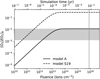 |
Fig. 2 Simulation results of [O3]/[O2]0 irradiated by 5 keV protons at 12 K, based on model A (solid line) and model S19 (dashed line). The shaded gray region shows the range of steady-state [O3]/[O2]0 obtained by Ennis et al. (2011) with an uncertainty of a factor of three. The vertical gray line indicates the fluence of 7.6 × 10¹⁵ ions cm−2 which was required to reach the steady state in the experiment of Ennis et al. (2011). |
3.2.2 Pure O2 ice
Figure 2 shows the simulation results of proton-irradiated pure O2 ice at 12 K obtained with model A. The steady-state [O3]/[O2]0 is 1.19%, which is roughly consistent with the experimental results. However, the fluence required to reach the steady state is approximately two orders of magnitude smaller than the experimental values. In this simulation, O3 is mainly formed via the nondiffusive reaction
![Mathematical equation: $\[\mathrm{O}^*+\mathrm{O}_2 \longrightarrow \mathrm{O}_3\]$](/articles/aa/full_html/2026/04/aa58232-25/aa58232-25-eq52.png) (R13)
(R13)
and the quenching of O3*. It is mainly destroyed by radiolysis, with minor contributions from the reactions
![Mathematical equation: $\[\mathrm{O}_2^*+\mathrm{O}_3 \longrightarrow 2 ~\mathrm{O}_2+\mathrm{O},\]$](/articles/aa/full_html/2026/04/aa58232-25/aa58232-25-eq53.png) (R14)
(R14)
![Mathematical equation: $\[\mathrm{O}^*+\mathrm{O}_3 \longrightarrow 2 ~\mathrm{O}_2.\]$](/articles/aa/full_html/2026/04/aa58232-25/aa58232-25-eq54.png) (R15)
(R15)
3.3 Model results using the SVHC19 network
As shown in Section 2.2, the chemical network of model A differs slightly from that used in SVHC19. Hereafter, we refer to the model based on their network as S19. We briefly summarize the differences below.
We set the branching ratios of the H + O2H reactions to 0.2, 0.2, and 0.6 for the pathways that produce OH + OH, O2 + H2, and H2O2, respectively, according to Cuppen et al. (2010); Lamberts et al. (2013), while in model S19, these values are 0.0194, 0.0857, and 0.894, respectively;
For the H + H2O2 reactions, we adopted branching ratios and activation barriers of 0.5 and 3400 K, respectively, for the reaction H + H2O2 ⟶ H2O + OH, and 0.5 and 4200 K for the reaction H + H2O2 ⟶ O2H + H2 (Ellingson et al. 2007; Lamberts et al. 2013, 2016; Lamberts & Kästner 2017; Lu et al. 2018, 2019), while in S19, the values are 0.999 and 1400 K for the former reaction and 0.0006 and 1900 K for the latter reaction;
We set the activation barriers for the O + O2 ⟶ O3/O3* reactions to 300 K, while S19 adopts 180 K for O + O2 ⟶ O3 and 0 K for O + O2 ⟶ O3*. We modified this value to reduce the formation of O3 and O3*, and it lies within the range estimated from the experiment of Benderskii & Wight (1996);
We set the branching ratios of the O* + O2 reactions to 0.05, 0.90, and 0.05 for the reactions that produce O3, O + O2, and O3*, respectively, while in S19, the values are all 0.333. We made this modification to reduce the formation of O3 and O3*;
We set the activation barrier of the OH + H2O2 ⟶ H2O + O2H reaction to 220 K, while S19 uses 760 K. We modified this barrier to increase the destruction of H2O2, and our value is reasonable according to Atkinson et al. (2004); Buszek et al. (2012);
We added a pathway to the O2H + O2H reaction that produce H2O + O3 (Zhang et al. 2011) with a branching ratio of 0.1, in addition to the H2O2 + O2 pathway in S19. Silva et al. (2025) report that the branching ratio of the H2O + O3 pathway is 0.19. Here, we adjusted it to 0.1 to better fit the experiments. Adding this pathway reduces the formation of H2O2, especially at 77 K.
Branching ratios, reaction activation energies, and chemical pathways all have substantial uncertainties. For activation energies, we examined all references in the NIST chemical kinetics database1, which show variations in values from different experiments and theoretical calculations. The exact values adopted in model A were tuned to obtain better agreement with the experimental results (see also Section 4.1). We used model S19 to simulate proton-irradiated H2O and O2 ice to demonstrate how these changes in activation barriers and branching ratios affect the simulation results.
3.3.1 Pure H2O ice
Figure 3 shows the simulation results for proton-irradiated pure H2O ice at 16 K and 77 K with model S19. Similar to model A, the steady state is reached at ~3 × 10¹³ ions cm−2, earlier than in the experiment. However, model S19 results in [H2O2]/[H2O] = 42.7% at 16 K and 14.1% at 77 K, both significantly higher than the experimental results. The higher [H2O2]/[H2O] abundance ratio in model S19 compared with model A is likely due to the higher activation barrier of reaction R12, which is 760 K in model S19 and 220 K in model A. At 16 K, H2O2 is mainly destroyed by the radiolysis reactions rather than by R12, which is the major destruction reaction in model A. At 77 K, although the higher dust temperature allows the activation barrier to be overcome, the reaction rate of R12 remains lower in model S19 than that in model A, and radiolysis reactions contribute more to the destruction of H2O2 in model S19. The major formation reactions of H2O2 at 16 K are nondiffusive reactions:
![Mathematical equation: $\[\mathrm{OH}+\mathrm{OH} \longrightarrow \mathrm{H}_2 \mathrm{O}_2,\]$](/articles/aa/full_html/2026/04/aa58232-25/aa58232-25-eq55.png) (R16)
(R16)
R7, R11, R10, and R9. At 77 K, H2O2 forms primarily by reaction R8, with minor contributions from reactions R11 and R9.
3.3.2 Pure O2 ice
Figure 2 shows the simulation results for proton-irradiated O2 ice. Generally, the results of model S19 follow a similar trend to those of model A, but the steady-state [O3]/[O2]0 is 29.6%, much higher than the experimental results. The activation barriers of reactions
![Mathematical equation: $\[\mathrm{O}+\mathrm{O}_2 \longrightarrow \mathrm{O}_3\]$](/articles/aa/full_html/2026/04/aa58232-25/aa58232-25-eq56.png) (R17)
(R17)
![Mathematical equation: $\[\mathrm{O}+\mathrm{O}_2 \longrightarrow \mathrm{O}_3{}^*\]$](/articles/aa/full_html/2026/04/aa58232-25/aa58232-25-eq57.png) (R18)
(R18)
are lower in model S19 than in model A, which boosts the formation of O3. Another difference between models A and S19 is the branching ratios of reactions,
![Mathematical equation: $\[\mathrm{O}^*+\mathrm{O}_2 \longrightarrow\left\{\begin{array}{l}\mathrm{O}_3 \\\mathrm{O}+\mathrm{O}_2, \\\mathrm{O}_3{}^*\end{array}\right.\]$](/articles/aa/full_html/2026/04/aa58232-25/aa58232-25-eq58.png) (R19)
(R19)
which are all 0.333 in model S19, and 0.05, 0.90, and 0.05 in model A. This further increases the steady-state [O3]/[O2]0 in model S19. The destruction reactions of O3 in model S19 are
![Mathematical equation: $\[\mathrm{O}_3{}^*+\mathrm{O}_3 \longrightarrow 3 ~\mathrm{O}_2,\]$](/articles/aa/full_html/2026/04/aa58232-25/aa58232-25-eq59.png) (R20)
(R20)
radiolysis reactions, R15, and R14.
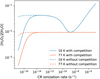 |
Fig. 4 Simulation results of the steady-state [H2O2]/[H2O] abundance ratio in model A as a function of the CR ionization rate. Results at 16 K and 77 K are shown with blue and orange lines, respectively. The solid and dashed lines indicate the results with and without reaction-diffusion competition, respectively. |
3.4 Sensitivity to the CR ionization rates
Most experiments study H2O radiolysis using CR fluxes of ~109−1012 ions s−1 cm−2 (Moore & Hudson 2000; Gomis et al. 2004b,a; Mejía et al. 2022), corresponding to CR ionization rates of ~10−9−10−6 s−1, due to instrument limitations and experiment duration. Their results show that the steady-state [H2O2]/[H2O] abundance ratio is, though not perfectly, independent of the CR flux in the experiment (Moore & Hudson 2000; Gomis et al. 2004b,a; Mejía et al. 2022). Figure 4 shows the steady-state [H2O2]/[H2O] from model A as a function of the CR ionization rate at 16 K and 77 K. At both temperatures, [H2O2]/[H2O] increases with the CR ionization rates when ζ ≲ 10−14 s−1. At higher ζ, the 77 K model predicts a constant [H2O2]/[H2O], whereas the 16 K model exhibits a complex variation in [H2O2]/[H2O]. The ratio decreases to a local minimum at ζ ~ 10−9−10−8 s−1 and then increases monotonically at higher ζ. However, the [H2O2]/[H2O] ratios in the range 10−9 s−1 < ζ < 10−6 s−1 vary roughly by a factor of two to three around ~2%, which is lower than the experimental uncertainties.
Similarly, Figure 5 shows the [O3]/[O2]0-ζ plot of model A. The [O3]/[O2]0 abundance ratio decreases with the CR ionization rate. Within the experimental range of CR flux, i.e., 10−9 s−1 < ζ < 10−6 s−1, the variation of the ratio is small. Therefore, we conclude that model A successfully reproduces the constant steady-state abundance ratios within the experimental range of CR flux in both the H2O and O2 experiments.
3.5 Sensitivity of H2O radiolysis to G-values
The G-values listed in Table 1 depend on several factors and assumptions, including the intermediate pathways considered in the radiolysis process. Shingledecker et al. (2018) adopted G-values of 3.704 for type R1 radiolysis and 1.747 for types R2 and R3. In contrast, SVHC19 adopted 0.257 for type R1 and 0.158 for types R2 and R3. The higher values represent the number of the dissociated H2O after every 100 eV deposited, whereas the lower values provide “effective” G-values that implicitly include reformation processes of H2O to compensate for those potentially underrepresented in the model. Because our model ignores the chemical effects of charged species, we may have missed some radiolysis pathways, leading to an overestimate of the G-values.
Our model A overestimates the destruction of H2O (see Section 3.2.1). Here, we test the sensitivity of the simulation results to the uncertainties in the G-values of H2O radiolysis by lowering them by one order of magnitude to determine whether this significantly reduces the destruction of H2O while maintaining a significant amount of H2O2 production. Figure 6 illustrates the results. At 16 K, the steady-state [H2O2]/[H2O] is 1.71%, remaining consistent with the experimental values. In this case, 22% of the initial H2O is destroyed, which is lower than in model A and closer to the experimental values, resulting in steady-state [H2]/[H2O] and [O2]/[H2O] ratios of 26.8% and 11.4%, respectively. At 77 K, the steady-state [H2O2]/[H2O] is 1.65%, slightly higher than in model A and the experimental value. About 20% of the initial H2O is destroyed. These results demonstrate that lowering the G-values of H2O radiolysis reduces H2O destruction and brings the simulation results closer to the experimental values, while the [H2O2]/[H2O] ratio remains roughly consistent with the experiments.
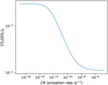 |
Fig. 5 Simulation results of the steady-state [O3]/[O2]0 abundance ratio in model A as a function of the CR ionization rate. |
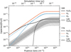 |
Fig. 6 Same as Figure 1, but for model A with the G-values of H2O radiolysis lowered by one order of magnitude. |
3.6 Effects of reaction-diffusion competition
As described in Section 2.1, the reaction-diffusion competition mechanism was introduced into the Nautilus code to increase the likelihood of reactions with finite activation barriers (Chang et al. 2007; Garrod & Pauly 2011; Ruaud et al. 2016). In contrast, the SVHC19 model does not include this competition. Figure 4, shows the [H2O2]/[H2O]-ζ plot for model A without reaction-diffusion competition, for comparison with the case with the results that include the competition. At both 16 K and 77 K, models without competition produce higher [H2O2]/[H2O] at ζ ≲ 10−14 s−1 compared with the case that includes the competition. For ζ ≳ 10−14 s−1, the results of the two cases are consistent.
To explore the differences in [H2O2]/[H2O] ratios at ζ ≲ 10−14 s−1 between models with and without competition, we examined the major formation and destruction reactions of H2O2 at low ζ. We find that these reactions match those at high ζ, i.e., formation via R7, R8, R9, R10 and R11, and destruction by R12. All formation reactions are without activation barriers, whereas the destruction reaction, R12, has a barrier of 220 K in model A. Thus, including the reaction-diffusion competition increases the destruction rate of H2O2, resulting in a lower [H2O2]/[H2O]. At higher ζ, the abundance of OH increases significantly because faster radiolysis of H2O boosts OH formation. Abundant OH rapidly destroys H2O2, so the steady-state [H2O2]/[H2O] depends on the formation rate of H2O2 rather than its destruction. Consequently, the reaction-diffusion competition no longer affects [H2O2]/[H2O] at high ζ. This interpretation is further supported by the fact that, at low ζ, OH is only destroyed via reaction R12, whereas at high ζ, reactions with H and O2H also contribute to OH destruction. Thus, at low ζ, OH is scarce and is consumed entirely by H2O2, whereas at high ζ, OH is abundant and can both destroy H2O2 and participate in the destruction of H and O2H. Such abundant OH at high ζ renders reaction R12 no longer limited by the activation barrier, so the reaction-diffusion barrier no longer affects H2O2 destruction.
The inclusion of the reaction-diffusion competition does not affect the simulation results in the O2 experiment. Therefore, we do not show these results in Figure 5.
3.7 Effects of nondiffusive chemistry
All reactions that lead to the formation and destruction of H2O2 are nondiffusive reactions. Figure 7 shows the simulation results of model A with all nondiffusive reaction removed. The steady-state [H2O2]/[H2O] abundance ratio is extremely low (~10−20) at 16 K, but 0.736% at 77 K. These results indicate that nondiffusive chemistry is crucial for H2O2 formation at 16 K. However, at 77 K, the [H2O2]/[H2O] ratio does not differ significantly from that of model A (0.941%). In this case, H2O2 forms through the reaction
![Mathematical equation: $\[\mathrm{H}+\mathrm{O}_2 \mathrm{H} \longrightarrow \mathrm{H}_2 \mathrm{O}_2 \text {. }\]$](/articles/aa/full_html/2026/04/aa58232-25/aa58232-25-eq60.png) (R21)
(R21)
The formation of O2H relies on the reaction between two O-bearing species, and is therefore slow at 16 K but fast at 77 K, as higher temperatures allow the O-bearing species to diffuse on the dust grain before reacting.
3.8 Sensitivity to the desorption energies of suprathermal species
The desorption energies (ED) of mantle species can also affect the simulation results. For diffusive reactions, the rate coefficient depends on exp(−Ediff/Tice), where Ediff = 0.7ED, except for H and H2. It also depends on the characteristic vibrational frequencies of the reactants, with ![Mathematical equation: $\[\nu \propto \sqrt{E_{\mathrm{D}}}\]$](/articles/aa/full_html/2026/04/aa58232-25/aa58232-25-eq61.png) . For nondiffusive reactions, the rate coefficient depends only on ν. The ED values of the suprathermal species are unknown due to the lack of experiments and are assumed to be the same as those of the corresponding thermal species. In this section, we explore the possible effect of changing the ED of the suprathermal species. We conducted several tests, arbitrarily lowering the ED of one suprathermal species at a time by an order of magnitude based on model A, because suprathermal species are more active than thermal species. Figure 8 shows the resulting [H2O2]/[H2O] variations relative to model A. At 16 K, the results show that the [H2O2]/[H2O] ratio is not sensitive to the change in the ED of the suprathermal species. At 77 K, lowering the ED of O*, OH*, and H2O* enhances [H2O2]/[H2O] by a factor of approximately three. In addition, changing the ED of H* reduces [H2O2]/[H2O] to ~10−4 times the value in model A. Therefore, the simulation results are sensitive to the ED values of certain suprathermal species under specific conditions; however, relevant experimental data remain scarce.
. For nondiffusive reactions, the rate coefficient depends only on ν. The ED values of the suprathermal species are unknown due to the lack of experiments and are assumed to be the same as those of the corresponding thermal species. In this section, we explore the possible effect of changing the ED of the suprathermal species. We conducted several tests, arbitrarily lowering the ED of one suprathermal species at a time by an order of magnitude based on model A, because suprathermal species are more active than thermal species. Figure 8 shows the resulting [H2O2]/[H2O] variations relative to model A. At 16 K, the results show that the [H2O2]/[H2O] ratio is not sensitive to the change in the ED of the suprathermal species. At 77 K, lowering the ED of O*, OH*, and H2O* enhances [H2O2]/[H2O] by a factor of approximately three. In addition, changing the ED of H* reduces [H2O2]/[H2O] to ~10−4 times the value in model A. Therefore, the simulation results are sensitive to the ED values of certain suprathermal species under specific conditions; however, relevant experimental data remain scarce.
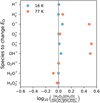 |
Fig. 8 Logarithm of the ratio between the simulated [H2O2]/[H2O] obtained after lowering the desorption energy of a specific suprathermal species by an order of magnitude and the simulated [H2O2]/[H2O] in model A. Results at 16 K are shown in blue and those at 77 K are shown in orange. The vertical gray line indicates the positions where [H2O2]/[H2O] is unchanged after modifying the desorption energy. The ratio obtained by changing the ED of H* at 77 K is −3.86, far outside the range of the x-axis, and is therefore not plotted. |
4 Discussion
4.1 Comparison with Shingledecker et al. (2019)
Model A successfully reproduces the steady-state [H2O2]/[H2O] in the H2O experiment and the [O3]/[O2]0 in the O2 experiment, although it underestimates the ion fluence required to reach the steady state. However, using the SVHC19 network fails to reproduce the experiments despite employing the same chemical network and radiolysis formalism, quenching of suprathermal species, and nondiffusive chemistry. The S19 model overproduces H2O2 in the H2O experiment (Figure 3) and O3 in the O2 experiment (Figure 2). As stated in Section 2.2, our models differ in several aspects. The main difference is that SVHC19 included the modified rate equations to account for stochastic effects in surface chemistry, as proposed by Garrod (2008). However, these modified rates should only influence the model results in the limit accretion case (when the number of reactants on the surface is close to one), which does not apply to our case. We also used a different electronic stopping power than SVHC19, which resulted in different radiolysis rates. In addition, there may be different treatments or slightly different surface parameters between the two models, which are difficult to assess. However, in their best model, SVHC19 produced negligible amounts of O2 when simulating H2O radiolysis. This is likely because they used “effective” G values, which are lower than the destruction G values that account for the reformation processes of H2O not considered in the model.
To bring the simulated results closer to the experimental data, we modified the reaction network based on that used in SVHC19, as introduced in Section 3.3. By increasing the activation barriers of the O + O2 ⟶ O3/O3* reactions and the branching ratios of the O* + O2 reactions, we produce less O3 (and O3*) in the O2 experiment compared with the SVHC19 network. By lowering the activation barrier of reaction R12 from 760 K in model S19 to 220 K in model A, we make it the major destruction reaction of H2O2. Simultaneously, we added a new pathway for the O2H + O2H reaction to reduce the formation rate of H2O2. These changes reduce the [H2O2]/[H2O] and [O3]/[O2]0 ratios of model S19, bringing model A into agreement with the experiments.
The comparison between models A and S19 highlights the importance of activation barriers and branching ratios in the chemical network. In such a small network designed to reproduce the radiolysis experiment of pure ices, the exact values of the activation energies and the branching ratios for certain reactions can completely alter the steady-state abundances. For example, by adding the reaction pathway O2H + O2H ⟶ H2O + O3 with a branching ratio of 0.1 and reducing the branching ratio of reaction O2H + O2H ⟶ H2O2 + O2 (R8) to 0.9, the steady-state [H2O2]/[H2O] decreases by a factor of approximately eight (from 7.11% to 0.941%; not shown in Section 3). Many of the activation barriers and branching ratios, if not all, are poorly or completely unknown for surface reactions. Indeed, the values for which we have estimates and references were obtained for the gas phase at room temperature and can be much lower in ices. For example, the activation energy of CO + O in the gas phase at room temperature is between 2500 and 3000 K (Talbi et al. 2006), but only 627 K in ices (Minissale et al. 2013). Consequently, we did not test all parameters to achieve perfect agreement with the experiments. Furthermore, the desorption energies of the suprathermal species, which are also poorly constrained experimentally, can also affect the simulation results.
4.2 Uncertainties in G-values of H2O radiolysis
In this study, we consider only three radiolysis processes (see Section 2.1) and neglect the production of charged species on dust grains. The grains in MCs are generally thought to be negatively charged, so molecular ions adsorbed or formed on dust grains rapidly recombine with the electrons on the dust surface (Umebayashi & Nakano 1980; Aikawa et al. 1999). However, it remains unclear whether the molecular ions in the bulk ice can react with other species. Kinetic simulation of ion chemistry on the surface and in the bulk is challenged by the lack of theoretical calculations and experiments of negatively charged dust grains (Cui & Herbst 2024). We note that charged particles, such as H2O+, H3O+, OH−, and e− (Muroya et al. 2005; Baragiola et al. 2008; Teolis et al. 2017), can be produced during radiolysis and play an important role in chemical evolution, particularly in H2O radiolysis. Experiments indicate that H2O is resistant to ion irradiation, rapidly reforming after dissociation (Le Caër 2011). Neglecting these species and processes may cause model A to overestimate both the extent and the rate of H2O destruction. By arbitrarily reducing the G-values of H2O radiolysis by an order of magnitude (see Section 3.5), i.e., taking into consideration an “effective” destruction rate lower than the primary destruction induced by the impinging ion, the simulation results better match the experiments, particularly regarding the fluence required to reach the steady state. Therefore, the lack of details about the intermediate pathways in the radiolysis processes may explain why we were unable to obtain the same evolution trend of [H2O2]/[H2O] as the experiments. This test model highlights the importance of understanding these pathways and implementing them in chemical models. Further studies on the ion chemistry in dust grains are thus needed.
4.3 Testing formalism for surface and bulk processes
The chemistry in both the gas phase and on grain surfaces is treated using the rate-equation approach. Although valid for gas-phase processes, this treatment is a strong approximation for reactions at the surface of the grains and in the grain mantles. The original equations of Hasegawa et al. (1992) do not account for the random walk of species on grains or the possibility that they remain in the same position longer, which increases the probability that a reaction occurs despite its activation energy. Chang et al. (2007) and Garrod & Pauly (2011) proposed a modification to compute reaction probabilities, commonly called “competition between reaction and diffusion.” In this study, we tested the effect of this modification to better reproduce the experimental results for the irradiation of pure water ices. Model A initially includes competition; we find that its removal increases the steady-state [H2O2]/[H2O] at low ζ (≲10−14 s−1) because competition facilitates H2O2 destruction through reaction R12, which has an activation barrier of 220 K. At higher ζ, the competition does not affect the steady-state [H2O2]/[H2O].
Another recent addition to astrochemical models is the treatment of nondiffusive chemistry. This process accounts for the fact that when two species are produced nearby on grains (e.g., by radiolysis), they can react directly without diffusing. Our test models indicate that nondiffusive chemistry is essential for the formation of H2O2 in the H2O radiolysis experiments, particularly at low temperatures where diffusive reactions of O-bearing species are inefficient. In their studies, SVHC19 and Jin & Garrod (2020) propose two very different formalisms to implement nondiffusive chemistry in models. In this work, we tested the effects of both formalisms on the model results. However, when using the reduced network, the formalism of Jin & Garrod (2020) failed to converge. In this formalism, the nondiffusive reaction rate is a sum of two terms, one of which is not proportional to the abundance of a reactant. This implies that if one of the reactants is insufficiently produced, its destruction rate may exceed its formation rate. In a larger network, with many processes, this situation may not occur. Non-diffusive chemistry is therefore the most important process for reproducing experiments at low temperatures.
4.4 Effect of the CR ionization rate
As shown in Section 3.4, model A produces nearly constant [H2O2]/[H2O] and [O3]/[O2]0 within the range of CR fluxes used in the experiments (~109−1012 ions s−1 cm−2, corresponding to ζ ~ 10−9−10−6 s−1). However, the typical values of ζ in interstellar MCs are ~10−17−10−16 s−1, significantly lower than the experimental values. Figures 4 and 5 indicate that the efficiency of radiolysis differs between these two ranges of ζ. Although the reaction network is rather simplified, the steady-state [H2O2]/[H2O] and [O3]/[O2]0 are still not proportional to ζ. We also note that modifications to the network (e.g., activation barriers and branching ratios of specific reactions) also affect how the steady-state [H2O2]/[H2O] evolves with ζ. For example, reducing the barriers of the O + O2 reactions makes the [H2O2]/[H2O] sink at 16 K and ζ ~ 10−9 s−1 in Figure 4 shallower (not shown). It remains unclear when and why the [H2O2]/[H2O]-ζ curve changes in response to modifications of activation barriers for specific reactions. Because of these complexities, it is difficult to fully interpret our results and use them to explain the observations of the real MCs.
5 Conclusions
Radiolysis has been proposed as an important process for the formation of prebiotic molecules in the interstellar environment. In this work, we attempted to reproduce the experiments of proton-irradiated pure H2O (Gomis et al. 2004a) and O2 (Ennis et al. 2011) ice using the Nautilus code, a complex gas-grain astrochemical code that includes radiolysis reactions, quenching of suprathermal species, reactions between suprathermal and thermal species, and nondiffusive reactions.
Model A, based on the SVHC19 network with modifications to certain activation barriers and branching ratios, successfully reproduces the steady-state [H2O2]/[H2O] in the H2O experiment and the [O3]/[O2]0 in the O2 experiment. It also produces nearly constant [H2O2]/[H2O] and [O3]/[O2]0 ratios across the experimental CR flux range, in agreement with the experimental findings. However, it underestimates the ion fluence required to reach the steady state in both the H2O and O2 experiments. Additionally, it overestimates the destruction of H2O, and the steady-state [H2]/[H2O] and [O2]/[H2O] in the H2O experiment.
We also conducted several tests based on model A to examine how the G-values of H2O radiolysis, reaction-diffusion competition, nondiffusive chemistry, and the desorption energies of suprathermal species affect the simulation results of the H2O experiment. By lowering the G-values of H2O radiolysis by an order of magnitude, to account for potentially insufficiently considered reformation processes from ions produced by radiolysis in the network, the destruction of H2O is reduced, bringing the simulation results closer to experimental values. Neglecting these reformation processes may explain why we could not reproduce the evolution trend of the observed abundance ratios. The reaction-diffusion competition is included in model A, and its removal increases the [H2O2]/[H2O] at low ζ (≲10−14 s−1) because this competition facilitates the destruction of H2O2 by OH. Nondiffusive reactions dominate the formation and destruction of H2O2; removing nondiffusive chemistry in model A strongly hampers the formation of H2O2 at 16 K but has minimal effect at 77 K. The simulation results are insensitive to the desorption energies of the suprathermal species at 16 K, but are sensitive to the desorption energies of H*, O*, O3*, and OH* at 77 K.
Our simulation results show that the steady-state [H2O2]/[H2O] and [O3]/[O2]0 in radiolysis experiments can be reproduced by fine-tuning the chemical model. More experiments are needed to determine the intermediate processes involved in radiolysis, particularly the ion chemistry in the ice bulk, as well as the activation barriers and branching ratios of the reactions in the network, which are crucial to improve our understanding of the radiolysis process through the chemical model.
The modified Nautilus code, with the inclusion of nondiffusive chemistry, radiolysis, and certain other processes, will be introduced in a forthcoming paper (Wakelam et al. in preparation) and will be made available at https://forge.oasu.u-bordeaux.fr/LAB/astrochem-tools/pnautilus.
Acknowledgements
The authors thank the anonymous referee for helpful comments. T.-Y. Tu acknowledges the financial support of the China Scholarship Council (No. 202406190190). V.W. acknowledges the CNRS program “Physique et Chimie du Milieu Interstellaire” (PCMI) co-funded by the Centre National d’Etudes Spatiales (CNES). Y.C. acknowledges the support from NSFC under grants Nos. 12121003, 12573047, and 12173018.
References
- Aikawa, Y., Herbst, E., & Dzegilenko, F. N. 1999, ApJ, 527, 262 [Google Scholar]
- Atkinson, R., Baulch, D. L., Cox, R. A., et al. 2004, ACP, 4, 1461 [Google Scholar]
- Bacmann, A., Taquet, V., Faure, A., Kahane, C., & Ceccarelli, C. 2012, A&A, 541, L12 [NASA ADS] [CrossRef] [EDP Sciences] [Google Scholar]
- Baragiola, R. A., Atteberry, C. L., Bahr, D. A., & Jakas, M. M. 1999, NIMPB, 157, 233 [Google Scholar]
- Baragiola, R. A., Famá, M., Loeffler, M. J., Raut, U., & Shi, J. 2008, NIMPB, 266, 3057 [Google Scholar]
- Baratta, G. A., Leto, G., & Palumbo, M. E. 2002, A&A, 384, 343 [NASA ADS] [CrossRef] [EDP Sciences] [Google Scholar]
- Benderskii, A. V., & Wight, C. A. 1996, JChPh, 104, 85 [Google Scholar]
- Bennett, C. J., Osamura, Y., Lebar, M. D., & Kaiser, R. I. 2005, ApJ, 634, 698 [Google Scholar]
- Bialy, S., Chemke, A., Neufeld, D. A., et al. 2026, NatAs [Google Scholar]
- Bisbas, T. G., Papadopoulos, P. P., & Viti, S. 2015, ApJ, 803, 37 [NASA ADS] [CrossRef] [Google Scholar]
- Bisbas, T. G., van Dishoeck, E. F., Papadopoulos, P. P., et al. 2017, ApJ, 839, 90 [Google Scholar]
- Boduch, Ph., Domaracka, A., Fulvio, D., et al. 2012, A&A, 544, A30 [NASA ADS] [CrossRef] [EDP Sciences] [Google Scholar]
- Bovino, S., Ferrada-Chamorro, S., Lupi, A., Schleicher, D. R. G., & Caselli, P. 2020, MNRAS, 495, L7 [Google Scholar]
- Bulak, M., Paardekooper, D. M., Fedoseev, G., et al. 2022, A&A, 657, A120 [NASA ADS] [CrossRef] [EDP Sciences] [Google Scholar]
- Buszek, R. J., Torrent-Sucarrat, M., Anglada, J. M., & Francisco, J. S. 2012, JPCA, 116, 5821 [Google Scholar]
- Caselli, P., Walmsley, C. M., Terzieva, R., & Herbst, E. 1998, ApJ, 499, 234 [Google Scholar]
- Chabot, M. 2016, A&A, 585, A15 [NASA ADS] [CrossRef] [EDP Sciences] [Google Scholar]
- Chang, Q., Cuppen, H. M., & Herbst, E. 2007, A&A, 469, 973 [NASA ADS] [CrossRef] [EDP Sciences] [Google Scholar]
- Cui, W., & Herbst, E. 2024, ACS Earth Space Chem., 8, 2218 [Google Scholar]
- Cuppen, H. M., Ioppolo, S., Romanzin, C., & Linnartz, H. 2010, PCCP, 12, 12077 [CrossRef] [Google Scholar]
- Dalgarno, A. 2006, PNAS, 103, 12269 [NASA ADS] [CrossRef] [Google Scholar]
- Dartois, E., Chabot, M., Id Barkach, T., et al. 2018, A&A, 618, A173 [NASA ADS] [CrossRef] [EDP Sciences] [Google Scholar]
- de Barros, A. L. F., Domaracka, A., Andrade, D. P. P., et al. 2011, MNRAS, 418, 1363 [NASA ADS] [CrossRef] [Google Scholar]
- Dewhurst, H. A., Dale, W. M., Bacq, Z. M., et al. 1952, Discuss. Faraday Soc., 12, 312 [Google Scholar]
- Ellingson, B. A., Theis, D. P., Tishchenko, O., Zheng, J., & Truhlar, D. G. 2007, JCPA, 111, 13554 [Google Scholar]
- Ennis, C. P., Bennett, C. J., & Kaiser, R. I. 2011, PCCP, 13, 9469 [Google Scholar]
- Gaches, B. A. L., & Viti, S. 2026, ACS Earth Space Chem., 10, 276 [Google Scholar]
- Garrod, R. T. 2008, A&A, 491, 239 [NASA ADS] [CrossRef] [EDP Sciences] [Google Scholar]
- Garrod, R. T., & Pauly, T. 2011, ApJ, 735, 15 [Google Scholar]
- Goldsmith, P. F., & Langer, W. D. 1978, ApJ, 222, 881 [Google Scholar]
- Gomis, O., Leto, G., & Strazzulla, G. 2004a, A&A, 420, 405 [NASA ADS] [CrossRef] [EDP Sciences] [Google Scholar]
- Gomis, O., Satorre, M. A., Strazzulla, G., & Leto, G. 2004b, P&SS, 52, 371 [Google Scholar]
- Hasegawa, T. I., & Herbst, E. 1993, MNRAS, 261, 83 [NASA ADS] [CrossRef] [Google Scholar]
- Hasegawa, T. I., Herbst, E., & Leung, C. M. 1992, ApJS, 82, 167 [Google Scholar]
- Hörl, E. M., & Kohlbeck, F. 1982, Acta Crystallogr. B: Struct. Crystallogr. Cryst. Chem., 38, 20 [Google Scholar]
- Hudson, R. L., & Moore, M. H. 1999, Icarus, 140, 451 [NASA ADS] [CrossRef] [Google Scholar]
- Indriolo, N., & McCall, B. J. 2012, ApJ, 745, 91 [NASA ADS] [CrossRef] [Google Scholar]
- Indriolo, N., & McCall, B. J. 2013, ChSRv, 42, 7763 [Google Scholar]
- Indriolo, N., Ivlev, A. V., Pellegrin, T., et al. 2026, ApJ, 997, 123 [Google Scholar]
- Ivlev, A. V., Röcker, T. B., Vasyunin, A., & Caselli, P. 2015, ApJ, 805, 59 [NASA ADS] [CrossRef] [Google Scholar]
- Jin, M., & Garrod, R. T. 2020, ApJS, 249, 26 [Google Scholar]
- Kalvāns, J. 2018, ApJS, 239, 6 [Google Scholar]
- Lamberts, T., Cuppen, H. M., Ioppolo, S., & Linnartz, H. 2013, PCCP, 15, 8287 [NASA ADS] [CrossRef] [Google Scholar]
- Lamberts, T., & Kästner, J. 2017, ApJ, 846, 43 [Google Scholar]
- Lamberts, T., Samanta, P. K., Köhny, A., & Kästner, J. 2016, PCCP, 18, 33021 [Google Scholar]
- Le Caër, S. 2011, Water, 3, 235 [Google Scholar]
- Léger, A., Jura, M., & Omont, A. 1985, A&A, 144, 147 [NASA ADS] [Google Scholar]
- Loeffler, M. J., Raut, U., Vidal, R. A., Baragiola, R. A., & Carlson, R. W. 2006, Icarus, 180, 265 [Google Scholar]
- Lu, X., Meng, Q., Wang, X., Fu, B., & Zhang, D. H. 2018, JChPh, 149, 174303 [Google Scholar]
- Lu, X., Wang, X., Fu, B., & Zhang, D. 2019, JPCA, 123, 3969 [Google Scholar]
- Mejía, C., de Barros, A. L. F., Rothard, H., Boduch, P., & da Silveira, E. F. 2022, MNRAS, 514, 3789 [CrossRef] [Google Scholar]
- Minissale, M., Congiu, E., Manicò, G., Pirronello, V., & Dulieu, F. 2013, A&A, 559, A49 [NASA ADS] [CrossRef] [EDP Sciences] [Google Scholar]
- Moore, M. H., & Hudson, R. L. 2000, Icarus, 145, 282 [Google Scholar]
- Mullikin, E., Anderson, H., O’Hern, N., et al. 2021, ApJ, 910, 72 [NASA ADS] [CrossRef] [Google Scholar]
- Muroya, Y., Lin, M., Wu, G., et al. 2005, RaPC, 72, 169 [Google Scholar]
- Neufeld, D. A., & Wolfire, M. G. 2017, ApJ, 845, 163 [Google Scholar]
- Neufeld, D. A., Welty, D. E., Ivlev, A. V., et al. 2024, ApJ, 973, 143 [Google Scholar]
- Neufeld, D. A., Silsbee, K., Ivlev, A. V., et al. 2026, ApJ, 998, 71 [Google Scholar]
- Öberg, K. I., Fuchs, G. W., Awad, Z., et al. 2007, ApJ, 662, L23 [Google Scholar]
- Obolentseva, M., Ivlev, A. V., Silsbee, K., et al. 2024, ApJ, 973, 142 [NASA ADS] [CrossRef] [Google Scholar]
- Padovani, M., Galli, D., & Glassgold, A. E. 2009, A&A, 501, 619 [NASA ADS] [CrossRef] [EDP Sciences] [Google Scholar]
- Palumbo, M. E., Strazzulla, G., Pendleton, Y. J., & Tielens, A. G. G. M. 2000, ApJ, 534, 801 [NASA ADS] [CrossRef] [Google Scholar]
- Paulive, A., Shingledecker, C. N., & Herbst, E. 2021, MNRAS, 500, 3414 [Google Scholar]
- Pilling, S., Seperuelo Duarte, E., da Silveira, E. F., et al. 2010, A&A, 509, A87 [NASA ADS] [CrossRef] [EDP Sciences] [Google Scholar]
- Pilling, S., Carvalho, G. A., & Rocha, W. R. M. 2022, ApJ, 925, 147 [NASA ADS] [CrossRef] [Google Scholar]
- Pilling, S., da Silveira, C. H., & Ojeda-Gonzalez, A. 2023, MNRAS, 523, 2858 [Google Scholar]
- Prasad, S. S., & Tarafdar, S. P. 1983, ApJ, 267, 603 [Google Scholar]
- Ruaud, M., Wakelam, V., & Hersant, F. 2016, MNRAS, 459, 3756 [Google Scholar]
- Rudd, M. E., Goffe, T. V., Dubois, R. D., Toburen, L. H., & Ratcliffe, C. A. 1983, PhRvA, 28, 3244 [Google Scholar]
- Seperuelo Duarte, E., Domaracka, A., Boduch, P., et al. 2010, A&A, 512, A71 [NASA ADS] [CrossRef] [EDP Sciences] [Google Scholar]
- Shen, C. J., Greenberg, J. M., Schutte, W. A., & van Dishoeck, E. F. 2004, A&A, 415, 203 [NASA ADS] [CrossRef] [EDP Sciences] [Google Scholar]
- Shingledecker, C. N., & Herbst, E. 2018, PCCP, 20, 5359 [Google Scholar]
- Shingledecker, C. N., Le Gal, R., & Herbst, E. 2017, PCCP, 19, 11043 [Google Scholar]
- Shingledecker, C. N., Tennis, J., Le Gal, R., & Herbst, E. 2018, ApJ, 861, 20 [Google Scholar]
- Shingledecker, C. N., Vasyunin, A., Herbst, E., & Caselli, P. 2019, ApJ, 876, 140 [Google Scholar]
- Silva, J. R. C., Queiroz, L. M. S. V., Ferrão, L. F. A., & Pilling, S. 2025, ApJ, 985, 254 [Google Scholar]
- Spitzer, Jr., L., & Tomasko, M. G. 1968, ApJ, 152, 971 [NASA ADS] [CrossRef] [Google Scholar]
- Talbi, D., Chandler, G. S., & Rohl, A. L. 2006, CP, 320, 214 [Google Scholar]
- Teolis, B. D., Plainaki, C., Cassidy, T. A., & Raut, U. 2017, JGRE, 122, 1996 [Google Scholar]
- Umebayashi, T., & Nakano, T. 1980, PASJ, 32, 405 [NASA ADS] [Google Scholar]
- Vasyunin, A. I., & Herbst, E. 2013, ApJ, 762, 86 [Google Scholar]
- Vasyunin, A. I., Caselli, P., Dulieu, F., & Jiménez-Serra, I. 2017, ApJ, 842, 33 [Google Scholar]
- Wakelam, V., Loison, J. C., Mereau, R., & Ruaud, M. 2017, MolAs, 6, 22 [NASA ADS] [Google Scholar]
- Wakelam, V., Dartois, E., Chabot, M., et al. 2021, A&A, 652, A63 [NASA ADS] [CrossRef] [EDP Sciences] [Google Scholar]
- Wakelam, V., Gratier, P., Loison, J. C., et al. 2024, A&A, 689, A63 [NASA ADS] [CrossRef] [EDP Sciences] [Google Scholar]
- Zhang, T., Wang, W., Zhang, P., Lü, J., & Zhang, Y. 2011, PCCP, 13, 20794 [Google Scholar]
- Zheng, W., Jewitt, D., & Kaiser, R. I. 2006, ApJ, 648, 753 [NASA ADS] [CrossRef] [Google Scholar]
- Ziegler, J. F., Ziegler, M. D., & Biersack, J. P. 2010, NIMPB, 268, 1818 [Google Scholar]
All Tables
Radiolysis processes considered in the simulations, including branching ratios, G-values, process types, and calculated stopping powers (10−14 eV cm2 molecule−1) for each species.
Reaction network considered here, based on Table 7 of Shingledecker et al. (2017).
All Figures
|
Fig. 1 Simulation results of abundance ratios [H2O2]/[H2O] (black lines), [H2]/[H2O] (orange lines), and [O2]/[H2O] (blue lines) with our model (model A) at 16 K (solid lines) and 77 K (dashed lines). The shaded gray and line-filled regions show the experimental results of [H2O2]/[H2O] by Gomis et al. (2004a) at 16 and 77 K, respectively, with an assumed uncertainty of a factor of three. |
| In the text | |
|
Fig. 2 Simulation results of [O3]/[O2]0 irradiated by 5 keV protons at 12 K, based on model A (solid line) and model S19 (dashed line). The shaded gray region shows the range of steady-state [O3]/[O2]0 obtained by Ennis et al. (2011) with an uncertainty of a factor of three. The vertical gray line indicates the fluence of 7.6 × 10¹⁵ ions cm−2 which was required to reach the steady state in the experiment of Ennis et al. (2011). |
| In the text | |
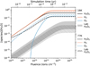 |
Fig. 3 Same as Figure 1, but for model S19. |
| In the text | |
|
Fig. 4 Simulation results of the steady-state [H2O2]/[H2O] abundance ratio in model A as a function of the CR ionization rate. Results at 16 K and 77 K are shown with blue and orange lines, respectively. The solid and dashed lines indicate the results with and without reaction-diffusion competition, respectively. |
| In the text | |
|
Fig. 5 Simulation results of the steady-state [O3]/[O2]0 abundance ratio in model A as a function of the CR ionization rate. |
| In the text | |
|
Fig. 6 Same as Figure 1, but for model A with the G-values of H2O radiolysis lowered by one order of magnitude. |
| In the text | |
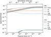 |
Fig. 7 Same as Figure 1, but for model A with all nondiffusive reactions removed. |
| In the text | |
|
Fig. 8 Logarithm of the ratio between the simulated [H2O2]/[H2O] obtained after lowering the desorption energy of a specific suprathermal species by an order of magnitude and the simulated [H2O2]/[H2O] in model A. Results at 16 K are shown in blue and those at 77 K are shown in orange. The vertical gray line indicates the positions where [H2O2]/[H2O] is unchanged after modifying the desorption energy. The ratio obtained by changing the ED of H* at 77 K is −3.86, far outside the range of the x-axis, and is therefore not plotted. |
| In the text | |
Current usage metrics show cumulative count of Article Views (full-text article views including HTML views, PDF and ePub downloads, according to the available data) and Abstracts Views on Vision4Press platform.
Data correspond to usage on the plateform after 2015. The current usage metrics is available 48-96 hours after online publication and is updated daily on week days.
Initial download of the metrics may take a while.