| Issue |
A&A
Volume 708, April 2026
|
|
|---|---|---|
| Article Number | L7 | |
| Number of page(s) | 6 | |
| Section | Letters to the Editor | |
| DOI | https://doi.org/10.1051/0004-6361/202558447 | |
| Published online | 31 March 2026 | |
Letter to the Editor
A cloudy fit to the atmosphere of WASP-107 b
1
Department of Astronomy, Tsinghua University, Haidian DS, 100084, Beijing, China
2
SRON Netherlands Institute for Space Research, Niels Bohrweg 4, 2333 CA, Leiden, The Netherlands
3
Space Telescope Science Institute, Baltimore, MD, USA
4
Kapteyn Astronomical Institute, University of Groningen, P.O. Box 800, 9700 AV, Groningen, The Netherlands
5
Leiden Observatory, Leiden University, P.O. Box 9513, 2300 RA, Leiden, The Netherlands
★ Corresponding author: This email address is being protected from spambots. You need JavaScript enabled to view it.
Received:
7
December
2025
Accepted:
8
March
2026
Abstract
Context. WASP-107 b has been observed comprehensively by JWST in the near- and mid-IR bands, meaning we can probe its composition and internal dynamics. Recent analyses reveal a 8 − 10 μm silicate feature, but it remains uncertain how silicate clouds form on this planet.
Aims. We aim to fit the complete JWST spectrum of WASP-107 b, from 0.9 μm to 12 μm with a physically motivated cloud model and self-consistent temperature profile.
Methods. We coupled two-stream radiative transfer to a cloud formation model until convergence between cloud and temperature profiles was reached. We searched a model grid that included metallicity, turbulent diffusivity, internal heat flux, and nucleation parameters to find the best-fit model.
Results. The silicate cloud feature at 10 μm and the near-IR molecular band strength can be simultaneously and naturally explained without assuming a parametrized temperature profile. A moderate vertical diffusivity of Kzz = 109 cm2 s−1 is needed to bring the cloud particles into the upper atmosphere of WASP-107 b. This Kzz is favored by the joint fitting of the near-IR water feature and mid-IR silicate feature – both of which are sensitive to clouds. Based on the strength of the H2O and CO2 bands, our model suggests a metallicity of 17 times solar.
Conclusions. Even in warm planets such as WASP-107 b, silicate clouds can form in the relatively cool upper atmosphere because turbulence uplifts vapor and cloud particles. Despite having considerably fewer degrees of freedom, the self-consistent modeling approach successfully fits WASP-107 b’s multiwavelength data, instilling confidence in the derived physical parameters.
Key words: planets and satellites: atmospheres / planets and satellites: gaseous planets / planets and satellites: individual: WASP-107 b
© The Authors 2026
 Open Access article, published by EDP Sciences, under the terms of the Creative Commons Attribution License (https://creativecommons.org/licenses/by/4.0), which permits unrestricted use, distribution, and reproduction in any medium, provided the original work is properly cited.
This article is published in open access under the Subscribe to Open model. This email address is being protected from spambots. You need JavaScript enabled to view it. to support open access publication.
1. Introduction
WASP-107 b is a warm, super-Neptune-mass planet around a K6 star. It has a size of 0.95 RJup and is on a 5.7-day orbit (Anderson et al. 2017). Follow-up radial velocity measurement refined its mass to 30.5 ± 1.7 M⊕ (Piaulet et al. 2021). WASP-107 b’s large radius makes it an ideal target for observing the transmission spectrum because the large planet-to-star radius ratio magnifies the spectral features. The Hubble Space Telescope (HST) transmission spectrum of this planet shows water features and cloud extinction in the near-IR (Kreidberg et al. 2018). Recently, JWST’s Near Infrared Camera (NIRCam) and Near InfraRed Spectrograph (NIRSpec) instruments found H2O, CO2, SO2, CO, NH3, and CH4 on WASP-107 b (Welbanks et al. 2024; Sing et al. 2024, W24W24 and S24S24 hereafter). Furthermore, JWST and HST have detected He absorption around the transit, indicating an ongoing atmospheric escaping process on this planet (Spake et al. 2018; Krishnamurthy et al. 2026, K25K25 hereafter).
With the observations from JWST, clouds on WASP-107 b are found at all wavelengths from 2.4 μm to 12 μm. S24 show that clouds are needed to lift the transit depth between 3.6 and 4.0 μm. Dyrek et al. (2024) find that the Mid-Infrared Instrument (MIRI) on board JWST clearly favors the presence of silicate clouds, whose Si-O stretching feature is hinted at 10 μm. Their retrieval suggests the presence of submicron-sized cloud particles at the ∼10−4 bar level. However, at those cool layers, it is believed that any silicates would have rained out to a deeper, hotter region. On the other hand, based on the depletion of CH4, the atmosphere of WASP-107 b is found to be strongly turbulent (S24), which could transport particles up into the visible atmosphere.
Most previous works fit the transmission spectrum of WASP-107 b with parameterized cloud properties. For example, S24 applied gray clouds and a power-law haze opacity to retrieve the 2.6–5.2 μm NIRSpec spectrum. Dyrek et al. (2024) used realistic optical properties of silicates but parameterized the vertical distribution of clouds. Also, W24 used an additional opacity with a skewed Gaussian shape along the wavelength dimension to mimic the mid-IR silicate opacity. Even though these cloud parameterizations provided successful fits to the spectra, the question of how silicate clouds form in the atmosphere of WASP-107 b has not yet been addressed.
Therefore, we investigated whether the cloud features on WASP-107 b can be understood with a realistic cloud formation model. Instead of parameterizing cloud properties, we simulated the cloud formation on WASP-107 b with the physically motivated cloud model ExoLyn (Huang et al. 2024). This allowed us to identify which silicate species the cloud particles are composed of. In addition, the temperature was calculated with a two-stream radiative transfer (RT) model that accounts for both molecular and cloud opacities (Huang et al., in prep.). We compared our model results with the transmission spectrum taken by JWST Near Infrared Imager and Slitless Spectrograph (NIRISS, K25), NIRCam (W24), and MIRI (Dyrek et al. 2024), covering near-IR to mid-IR wavelengths. Data at wavelengths λ < 1 μm and 2 − 2.5 μm were excluded as they may be affected by the transit light source effect (K25). The NIRCam data, from 2.5 μm to 5 μm, used in this study do not show evidence of a starspot crossing event (W24). Beyond λ > 2.5 μm the effect of starspots decreases with wavelength (Rackham et al. 2018). Therefore, the effect of a transit light source on our findings is minor.
2. Results
We coupled the cloud model ExoLyn with two-stream RT to get a self-consistent temperature-pressure (TP) profile and cloud structure. Our model is summarized in Appendix A, and the details are provided in Huang et al. (2024) and a companion paper. We constructed a grid of parameters (Table 1) with varying metallicity (Z), vertical turbulent diffusivity (Kzz), effective temperature of the internal emission flux (Tint), nucleus injection rate ( ), and nucleation depth (Pnuc) to find the parameters that best match the observations, including the mid-IR silicate features and the near-IR molecular band strength. For each parameter combination, we adjusted the equilibrium gas composition to account for the vertical mixing and sulfur photochemistry, which are described in Appendix A.2. The observational data from JWST/NIRISS (K25), JWST/NIRCam, and JWST/MIRI presented in W24 cover a broad wavelength range: 0.85–12 μm. The best-fit model is found with Z = 17 Z⊙, Kzz = 109 cm2 s−1, Tint = 550 K, Pnuc = 10−3 bar, and
  .
.
Parameters of the grid search.
The converged TP profile and the cloud structure are shown in Fig. 1. For the best-fit run, the upper cloud layer is dominated by SiO2, until 0.3 bar, where the dominant species changes to MgSiO3, Mg2SiO4, and Fe because SiO2 evaporates. Due to gravitational settling, the cloud mixing ratio peaks at 0.2 bar. Clouds evaporate at a pressure of 0.6 bar, where T ≈ 2200 K. At 2 × 10⁻³ bar and 5 × 10⁻³ bar, the atmosphere becomes optically thick to the stellar IR and visible photons. Here, the cloud particles reach sizes of ∼1 μm. Increasing Kzz does not change the dominant cloud species (SiO2) but does lead to more vertically extended clouds. This is because vapor gets replenished more efficiently in the cloud-forming region and the cloud particles are subject to a stronger updraft. The photospheric temperature we obtain (730 K) agrees with the retrieved values in K25 (∼700 K) and lies in between the radiative-convective-equilibrium models presented by W24 (∼500 K) and S24 (∼800 K).
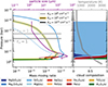 |
Fig. 1. Self-consistent temperature and cloud profiles resulting from the joint cloud and RT model. Left: Cloud profiles obtained for three Kzz values. The best-fit model has Kzz = 109 cm2 s−1 (the line with the golden highlight), and the corresponding particle size is shown by the purple line. The horizontal gray lines indicate the visible and IR photosphere. Right: Cloud composition by mass fraction of the best-fit model. The gray line shows the atmosphere temperature profile of the best fit. |
Figure 2 shows the synthetic transmission spectrum compared to observations. We also plot the simulation results obtained by varying the Kzz with respect to the best-fit model to demonstrate how this parameter affects the spectrum. Our model provides a good match to the strength of both the near-IR molecular bands and the mid-IR silicate feature. Compared to the clear spectrum, SiO2 clouds give rise to more absorption at 8 to 10 μm. In the near-IR, scattering by micron-sized particles raises the transit depth at wavelengths below 2.5 μm, suppressing the 1.2, 1.5, 1.9, and 2.8 μm H2O features. Besides H2O, other molecular features are also reproduced. The atmospheric metallicity affects the strength of the 4.4 μm CO2 feature and is constrained at ≈17 Z⊙. Our model also reproduces the SO2 feature at 7.4 μm under the assumption of a 9 × 10⁻³ conversion ratio from H2S to SO2. This conversion was applied to mimic the effects of photochemistry (not included in our model), which is believed to be the cause of SO2 on hot Jupiters (Tsai et al. 2023, W24).
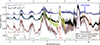 |
Fig. 2. JWST observations of WASP-107 b (colored vertical bars) along with the best-fit model (black line; Kzz = 109 cm2 s−1), resulting in a |

Varying the turbulent diffusivity parameter leads to vertical shifts in the transmission spectrum. When Kzz = 1010 cm2 s−1, clouds are more extended. In this case, cloud extinction of < 2 μm is too strong and the transit depth is overestimated compared to the observations. On the other hand, when Kzz = 108 cm2 s−1, clouds settle too deep, leading to a nearly invisible silicate feature and larger near-IR water line amplitudes. In conclusion, the cloud features at 1 − 4 μm and 8 − 10 μm can be reproduced only with a turbulent diffusivity Kzz = 109 cm2 s−1, consistent with the value inferred from the gas-phase disequilibrium chemistry model used in W24 and Changeat et al. (2025).
In Fig. 3 we show how the Kzz, Tint, and Z parameters change the spectroscopic features that are affected by clouds. To analyze the clouds’ ability to mute molecular lines, we measured the strength of the 1.4 μm H2O band. We used the water line strength metric from Stevenson (2016):
 (1)
(1)
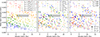 |
Fig. 3. Scatter plots demonstrating how the near-IR H2O line strength and the 10 μm silicate metric depend on the diffusivity parameter (Kzz; left), metallicity (Z; middle), and internal energy flux (Tint; right) model parameters. The size of the dots corresponds to the |

where ηwater is the transit depth at the peak of the H2O band (i.e., 1.36 − 1.44 μm) and ηcont is that at the continuum wavelengths (i.e., 1.22 − 1.3 μm). In addition to fwater, we quantified the strength of the 10 μm silicate feature through a silicate metric (fsilicate) obtained by decomposing the transmission spectrum from 8.4–10.1 μm into Legendre polynomials up to the second order: η(λ) = L0 + L1P1(λ)+L2P(λ). Then,
 (2)
(2)
where the asterisks indicate that L1 is limited to the range [ − 0.01L0, 0] and L2 < 0, respectively. The two terms encapsulate how the silicate feature manifests in the spectrum. Without silicates, the molecular opacity steeply decreases from 8–10 μm and fsilicate (through L1) becomes negatively. Silicate absorption reduces this decline: it flattens the opacity slope and increases fsilicate. With further increases of cloud thickness, a distinct absorption bump near 9 μm emerges, captured by L2. Defined in this way, the silicate metric provides substantial evidence for the presence of silicates when fsilicate takes a value ≳0.01. For WASP-107 b, the slope contribution (L1) dominates and fsilicate = 0.009, indicating the likely presence of silicates.
Although a large scatter is present in Fig. 3 due to the variation in parameters, a decreasing trend of fwater and a slightly increasing trend of fsilicate is identified with increasing Kzz. The stronger turbulence dredges up more vapor to the upper atmosphere, where it condenses to form silicates and to suppress the molecular features. Increasing the metallicity directly leads to a higher H2O abundance and stronger H2O features. On the other hand, the metallicity and Tint parameter do not influence fwater or fsilicate in a systematic way. However, a hotter interior promotes the quenching of CH4 in the upper atmosphere, resulting in better fits to JWST observations (as indicated by the size of the points): the average  of the top ten best-fit runs decreases from 4.3 to 3.8 when Tint increases from 350 K to 550 K. Three models lie within 1σ of the observational constraints on the silicate metric and the water metric. These points, all with
  , are statistically indistinguishable from the best-fit simulation. They all have parameters Kzz ≈ 109 cm2 s−1 and Z ≈ 17, confirming the robustness of our inferences.
Finally, the cloud profiles (and associated metrics) are mostly insensitive to nucleation parameters (not plotted). Higher nucleation rates are neutralized by coagulation, and turbulence efficiently spreads cloud nuclei vertically (Huang et al. 2024).
3. Conclusions and discussion
We investigated the cloud characteristics of WASP-107 b using a model strategy that couples a two-stream RT model and a physically motivated cloud formation model in a self-consistent manner. Our main findings are as follows:
-
The near-IR molecular band strength observed by JWST/NIRISS and NIRCam and the 10 μm silicate feature observed by JWST/MIRI can be reproduced simultaneously without assuming a parametrized cloud profile or temperature profile. Although the temperature in the upper atmosphere is relatively low compared to the condensation temperature of silicates, vertical updrafts lift cloud particles into the observable upper region.
-
The best-fit model employs a vertical turbulent diffusivity Kzz = 109 cm2 s−1, a typical value for exoplanet atmospheres (Kawashima & Min 2021; Baxter et al. 2021; Barat et al. 2025). When Kzz is lower, clouds become invisible due to gravitational settling, while a higher Kzz dredges up too much cloud material, inconsistent with the relatively weak silicate feature.
-
Turbulence governs both the amplitude of the 10 μm silicate feature and the strength of the near-IR water lines. Self-consistently modeling the effect of turbulence on clouds (thickness and intensity) allowed us to place tight constraints on Kzz.
The model used in this work eliminates excessive degrees of freedom compared to models that adopt a parametrized cloud opacity or TP profile. Despite consisting of just 1200 sets of parameters (Table 1), it is able to match the most prominent cloud features. With more and more JWST observations suggesting the presence of clouds on exoplanets (Grant et al. 2023; Inglis et al. 2024), the method could be applied in future (grid) retrievals.
Nevertheless, the 1D nature of the model is an assumption. Recently, differences in the morning versus evening limb spectrum of WASP-107 b have been pointed out (Murphy et al. 2024). The evening limb shows a stronger 2.7 μm H2O feature and a greater transit depth, which suggests an atmosphere that is 100 K hotter than the morning limb. The relatively weak 10 μm silicate feature may therefore only originate from the evening limb, as silicate clouds would likely rain out in the cooler morning limb. The limb asymmetry likely also affects the photochemistry related to the SO2 feature, as SO2 can only form on the dayside. A useful future effort would therefore be to integrate two limb models into our code, with different temperatures and compositions.
With its large radius relative to its mass, the super-puff WASP-107 b occupies a distinctive place in the exoplanet population. Similar to previous studies (S24 and W24), our modeling of the planet’s atmospheric indicates a high Tint, which suggests active internal heating driven by, for example, tidal or Ohmic dissipation (Batygin 2025; Tremblin et al. 2017). Notably, our inferred atmospheric metallicity of 17 times solar is consistent with the constraint in W24 but lower than the value reported by S24 – a finding that results from our self-consistent cloud model (see Appendix A.3). The slightly lower atmospheric metallicity leaves ample room for the bulk of the heavy elements to reside deep within the planet’s interior.
Acknowledgments
This work was supported by the National Natural Science Foundation of China (NSFC) project no. 12473065 and 12233004. The authors thank Kazumasa Ohno and Sharon Xuesong Wang for insightful discussion, and the anonymous referee whose comments substantially improved the quality of the paper.
References
- Allard, N. F., Spiegelman, F., Leininger, T., & Molliere, P. 2019, A&A, 628, A120 [NASA ADS] [CrossRef] [EDP Sciences] [Google Scholar]
- Anderson, D. R., Collier Cameron, A., Delrez, L., et al. 2017, A&A, 604, A110 [NASA ADS] [CrossRef] [EDP Sciences] [Google Scholar]
- Azzam, A. A. A., Tennyson, J., Yurchenko, S. N., & Naumenko, O. V. 2016, MNRAS, 460, 4063 [NASA ADS] [CrossRef] [Google Scholar]
- Barat, S., Désert, J.-M., Mukherjee, S., et al. 2025, AJ, 170, 165 [Google Scholar]
- Batygin, K. 2025, ApJ, 985, 87 [Google Scholar]
- Baxter, C., Désert, J.-M., Tsai, S.-M., et al. 2021, A&A, 648, A127 [NASA ADS] [CrossRef] [EDP Sciences] [Google Scholar]
- Borysow, A. 2002, A&A, 390, 779 [NASA ADS] [CrossRef] [EDP Sciences] [Google Scholar]
- Borysow, A., & Frommhold, L. 1989, ApJ, 341, 549 [NASA ADS] [CrossRef] [Google Scholar]
- Borysow, J., Frommhold, L., & Birnbaum, G. 1988, ApJ, 326, 509 [NASA ADS] [CrossRef] [Google Scholar]
- Borysow, A., Frommhold, L., & Moraldi, M. 1989, ApJ, 336, 495 [NASA ADS] [CrossRef] [Google Scholar]
- Borysow, A., Jorgensen, U. G., & Fu, Y. 2001, J. Quant. Spectr. Rad. Transf., 68, 235 [NASA ADS] [CrossRef] [Google Scholar]
- Changeat, Q., Bardet, D., Chubb, K., et al. 2025, A&A, 699, A219 [NASA ADS] [CrossRef] [EDP Sciences] [Google Scholar]
- Coles, P. A., Yurchenko, S. N., & Tennyson, J. 2019, MNRAS, 490, 4638 [CrossRef] [Google Scholar]
- Dominik, C., Min, M., & Tazaki, R. 2021, Astrophysics Source Code Library [record ascl:2104.010] [Google Scholar]
- Dyrek, A., Min, M., Decin, L., et al. 2024, Nature, 625, 51 [Google Scholar]
- Eddington, A. S. 1916, MNRAS, 77, 16 [NASA ADS] [Google Scholar]
- Grant, D., Lewis, N. K., Wakeford, H. R., et al. 2023, ApJ, 956, L29 [Google Scholar]
- Guillot, T. 2010, A&A, 520, A27 [NASA ADS] [CrossRef] [EDP Sciences] [Google Scholar]
- Henning, T., Begemann, B., Mutschke, H., & Dorschner, J. 1995, A&AS, 112, 143 [NASA ADS] [Google Scholar]
- Huang, H., Ormel, C. W., & Min, M. 2024, A&A, 691, A291 [NASA ADS] [CrossRef] [EDP Sciences] [Google Scholar]
- Inglis, J., Batalha, N. E., Lewis, N. K., et al. 2024, ApJ, 973, L41 [NASA ADS] [CrossRef] [Google Scholar]
- Jäger, C., Dorschner, J., Mutschke, H., Posch, T., & Henning, T. 2003, A&A, 408, 193 [NASA ADS] [CrossRef] [EDP Sciences] [Google Scholar]
- Kawashima, Y., & Min, M. 2021, A&A, 656, A90 [NASA ADS] [CrossRef] [EDP Sciences] [Google Scholar]
- Koike, C., Kaito, C., Yamamoto, T., et al. 1995, Icarus, 114, 203 [NASA ADS] [CrossRef] [Google Scholar]
- Kreidberg, L., Line, M. R., Thorngren, D., Morley, C. V., & Stevenson, K. B. 2018, ApJ, 858, L6 [Google Scholar]
- Krishnamurthy, V., Carteret, Y., Piaulet-Ghorayeb, C., et al. 2026, Nat. Astron., 10, 258 [Google Scholar]
- Leconte, J. 2021, A&A, 645, A20 [NASA ADS] [CrossRef] [EDP Sciences] [Google Scholar]
- Malik, M., Kitzmann, D., Mendonça, J. M., et al. 2019, AJ, 157, 170 [Google Scholar]
- McKemmish, L. K., Masseron, T., Hoeijmakers, H. J., et al. 2019, MNRAS, 488, 2836 [Google Scholar]
- Meador, W. E., & Weaver, W. R. 1980, J. Atmos. Sci., 37, 630 [NASA ADS] [CrossRef] [Google Scholar]
- Mihalas, D. 1978, Stellar Atmospheres (San Francisco: W.H. Freeman) [Google Scholar]
- Min, M., Hovenier, J. W., & de Koter, A. 2005, A&A, 432, 909 [NASA ADS] [CrossRef] [EDP Sciences] [Google Scholar]
- Mollière, P., Wardenier, J. P., van Boekel, R., et al. 2019, A&A, 627, A67 [Google Scholar]
- Murphy, M. M., Beatty, T. G., Schlawin, E., et al. 2024, Nat. Astron., 8, 1562 [NASA ADS] [CrossRef] [Google Scholar]
- Palik, E. D. 1991, Handbook of Optical Constants of Solids II (Boston: Academic Press) [Google Scholar]
- Piaulet, C., Benneke, B., Rubenzahl, R. A., et al. 2021, AJ, 161, 70 [NASA ADS] [CrossRef] [Google Scholar]
- Pollack, J. B., Hollenbach, D., Beckwith, S., et al. 1994, ApJ, 421, 615 [Google Scholar]
- Rackham, B. V., Apai, D., & Giampapa, M. S. 2018, ApJ, 853, 122 [Google Scholar]
- Rothman, L. S., Gordon, I. E., Barber, R. J., et al. 2010, J. Quant. Spectr. Rad. Transf., 111, 2139 [Google Scholar]
- Sing, D. K., Rustamkulov, Z., Thorngren, D. P., et al. 2024, Nature, 630, 831 [NASA ADS] [CrossRef] [Google Scholar]
- Spake, J. J., Sing, D. K., Evans, T. M., et al. 2018, Nature, 557, 68 [Google Scholar]
- Stevenson, K. B. 2016, ApJ, 817, L16 [NASA ADS] [CrossRef] [Google Scholar]
- Stock, J. W., Kitzmann, D., Patzer, A. B. C., & Sedlmayr, E. 2018, MNRAS, 479, 865 [NASA ADS] [Google Scholar]
- Stock, J. W., Kitzmann, D., & Patzer, A. B. C. 2022, MNRAS, 517, 4070 [NASA ADS] [CrossRef] [Google Scholar]
- Toon, O. B., Turco, R. P., Hamill, P., Kiang, C. S., & Whitten, R. C. 1979, J. Atmos. Sci., 36, 718 [NASA ADS] [CrossRef] [Google Scholar]
- Tremblin, P., Chabrier, G., Mayne, N. J., et al. 2017, ApJ, 841, 30 [NASA ADS] [CrossRef] [Google Scholar]
- Tsai, S.-M., Lee, E. K. H., Powell, D., et al. 2023, Nature, 617, 483 [CrossRef] [Google Scholar]
- Welbanks, L., Bell, T. J., Beatty, T. G., et al. 2024, Nature, 630, 836 [NASA ADS] [CrossRef] [Google Scholar]
- Yee, S. W., & Vissapragada, S. 2025, arXiv e-prints [arXiv:2511.07746] [Google Scholar]
- Yurchenko, S. N., Amundsen, D. S., Tennyson, J., & Waldmann, I. P. 2017, A&A, 605, A95 [NASA ADS] [CrossRef] [EDP Sciences] [Google Scholar]
- Yurchenko, S. N., Mellor, T. M., Freedman, R. S., & Tennyson, J. 2020, MNRAS, 496, 5282 [NASA ADS] [CrossRef] [Google Scholar]
- Yurchenko, S. N., Tennyson, J., Syme, A.-M., et al. 2022, MNRAS, 510, 903 [Google Scholar]
Appendix A: Methods
In this work, we computed the self-consistent cloud structure and temperature profile by coupling the multi-species cloud code ExoLyn with a two-stream RT method. Here we briefly summarize the physical principles of our simulations. Details of our RT model are described in the companion paper.
A.1. Coupling between cloud formation and radiative transfer
ExoLyn (Huang et al. 2024) is a 1D cloud formation model that solves for the composition, number density and size of the cloud particles. The cloud formation in ExoLyn is simulated as a chemical kinetics process instead of chemical equilibrium. For the cloud forming material, we assume C combines into CO and the leftover O forms H2O, which applies for the hot deep atmosphere. Due to turbulence (eddy diffusion), molecules are transported to cooler, upper layers and condense into clouds. The reaction rates at which condensates form are evaluated using the local vapor concentration and the thermo-chemical property of the cloud forming reactions. Once formed, a cloud particle is subject to sedimentation, turbulent diffusion and coagulation, until it evaporates in the bottom of the atmosphere. The steady state cloud profile is solved using a computationally efficient relaxation method. During the cloud formation process, gas-phase chemical reactions are neglected, for simplicity. After a cloud structure has been obtained, the remaining gas species are forced to chemical equilibrium using FastChem (Stock et al. 2018, 2022).
Cloud formation depends sensitively on the temperature structure of the atmosphere. Therefore instead of leaving the temperature structure as free parameters, we seek to solve for it self-consistently with cloud formation. The first step in the RT calculation is to compute the cloud and gas phase opacity structure. For the cloud opacity, we took the same setting as Huang et al. (2024). Effective medium theory (Bruggeman rule) was applied to the composition of the cloud particles to get the average (effective) refractive index of the material mixture. Then Optool (Dominik et al. 2021) was run to generate the cloud absorption and scattering opacity, assuming distribution of hollow spheres (DHS; Min et al. 2005) as the shape for the cloud particles. We used Exo-k (Leconte 2021) to mix the correlated-k tables of the individual gas species over the wavelength range from 0.3 μm to 50 μm, with a spectral resolution R = 300. The gas opacity sources included in the simulations are H2O, CH4, CO, CO2, NH3, H2S, Na, K, Mg, Fe, Al, SiO, TiO, and H2-H2, H2-He collisional induced absorption, summarized in Table A.1.
Opacity data used in this work.
Once the opacity was computed, we generalized the two-stream RT method in Guillot (2010) to get the temperature profile. The radiation field was decomposed into two components (Toon et al. 1979; Meador & Weaver 1980) – downward irradiation from the star in visible band and the upward irradiation from the planet interior in the IR band. For both the IR and visible components, moment equations (Mihalas 1978) were solved, with the addition of Eddington approximation as a closure condition (Eddington 1916). The location where the stellar energy is deposited is determined by the opacity distribution in the atmosphere, especially clouds, because they tend to absorb stellar visible photons efficiently. Applying energy balance – the radiation energy received by a layer equals the blackbody radiation it emits – the temperature at a certain layer was computed. The assumptions and simplifications in the above method are benchmarked against the RT code PICASO in the companion paper. The temperature gradient computed from radiation transfer becomes super-adiabatic in the deep atmosphere (≳0.1 bar). In reality, convection transports heat more efficiently in these regions and homogenizes the temperature. We corrected the super-adiabatic temperature gradient following the method presented in Malik et al. (2019), which guarantees that the temperature gradient is not larger than ∇ad (assumed to be 2/7) and the net energy flux is conserved throughout the atmosphere.
In this work, ExoLyn and the RT code were coupled iteratively. Starting from an initial temperature profile, we computed the cloud structure and then the gas and cloud opacity. After this, the temperature corresponding to the opacity structure was computed to update the guess temperature. This process was repeated iteratively until convergence in temperature was reached. In the end, we generated the transmission spectra with petitRADTRANS (Mollière et al. 2019).
A.2. Adjustment to the equilibrium chemistry
Before computing the transmission spectrum, we made several adjustments to the gas profile under chemical equilibrium. It was found that the gas composition on WASP-107 b is affected by disequilibrium chemistry such as photochemistry and quenching (W24). For example, the JWST transmission spectrum of WASP-107 b showed the signature of SO2, in contrast to H2S predicted by chemical equilibrium. The SO2 could be generated from oxidation of H2S in photochemical reactions. However, as the main focus of this work is to understand the cloud features on WASP-107 b with a microphysical model, running a photochemistry model is beyond the scope of the model. Therefore, we artificially converted some fraction of H2S to SO2.
In addition, at the temperature akin to WASP-107 b, the presence of CH4 and the absence of NH3 is expected by equilibrium chemistry. However, the observed underabundance of CH4 and overabundance of NH3 are signposts of disequilibrium chemistry, specifically vertical quenching. Under strongly turbulent conditions, CH4-poor gas from the deep atmosphere is dredged up into the visible, upper atmosphere, and vice versa, reducing the concentration of CH4. As simulating disequilibrium chemistry is beyond the scope of this work, we mimicked the above effects by postprocessing the gas profile before generating the transmission spectrum: we converted a fraction of fH2SH2S to SO2, and replaced all molecular abundances above a quenching pressure (Pquench) with those values at that location. For each parameter set in Table 1, the best-fit fH2S, Pquench and the reference pressure Pref at which the planet radius is measured are optimized by the conjugate gradient method. The best-fit parameters in Fig. 2 have fH2S = 9 × 10⁻³, Pquench = 0.06 bar.
Our model manages to fit the 7.2 μm SO2 feature, but undershoots the 4 μm SO2 feature. The reason could be that the cloud extinction in our model is slightly stronger than suggested by the 4 μm SO2 feature. Therefore, tuning a smaller Kzz could lead to a slightly clearer atmosphere and decrease the transit depth redward to the SO2 feature, providing a better fit. Note that the SO2 concentration in this work is calculated by simply converting 0.6% of H2S to SO2, translating to a nearly constant volume mixing ratio ≈10−6 at all locations in the atmosphere. W24 applied a 1D radiative-convective-photochemical equilibrium (RCPE) model, which found that SO2 only forms around a level of 10−5 bar, with the peak volume mixing ratio 10−4. Explaining the presence of SO2 with a cloudy RCPE model is left to a future work.
A.3. Higher-metallicity simulations
The best-fit atmospheric metallicity in our work, Z = 17 Z⊙, is consistent with the constraint from W24 (10 − 18 Z⊙) and with the K abundance from K25 ( ). However, it is lower than the values reported by S24 (43 ± 8 Z⊙). Motivated by their constraint, we simulated a metal-rich (Z = 56 Z⊙) and a low-metallicity (Z = 3.2 Z⊙) model to understand how metallicity affects the spectrum. The results are shown in Fig. A.1.
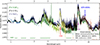 |
Fig. A.1. Same as Fig. 2 but with metallicity Z = 56 Z⊙ and Z = 3.2 Z⊙. For each metallicity, the control parameters (Appendix A.2) are kept the same as the best-fit model. |
With a  , the metal-rich atmosphere with Z = 56 Z⊙ offers a worse fit. Although a higher metallicity of 56 Z⊙ elevates the mean molecular weight to 3.07, its effect on the scale height is not strong enough to suppress the gas and cloud features. The amplitudes of the H2O features at 1.4 μm and the CO2 feature at 4.3 μm are overestimated compared to the observations. Increasing the metallicity results in a higher H2O abundance and enhances the corresponding features in the near-IR band. The CO2 abundance is especially sensitive to metallicity, with its signature at 4.3 μm enhanced from 400 ppm for 3.2 Z⊙ to 900 ppm for 56 Z⊙. The silicate feature at 10 μm is not sensitive to metallicity. Although more vapor condenses in a metal-rich atmosphere, the silicate-bearing cloud particles gravitationally settle to optically opaque layers once the particles grow larger.
The unusually large radius of WASP-107 b requires a large envelope mass fraction and small core mass of 5M⊕ (Piaulet et al. 2021). However, this poses a question to the formation theory how such a low mass core accreted an envelope of 25M⊕. The strong internal heating (Tint) inferred in our model, W24 and S24, suggests a hotter envelope and helps to explain the inflated radius of the planet without involving a small core mass fraction. This intense interior radiation potentially stems from the tidal heating related to the planet’s moderate eccentricity e ∼ 0.05 (Piaulet et al. 2021; Murphy et al. 2024; Yee & Vissapragada 2025) or from the Ohmic dissipation in the planet interior (Batygin 2025).
All Tables
All Figures
|
Fig. 1. Self-consistent temperature and cloud profiles resulting from the joint cloud and RT model. Left: Cloud profiles obtained for three Kzz values. The best-fit model has Kzz = 109 cm2 s−1 (the line with the golden highlight), and the corresponding particle size is shown by the purple line. The horizontal gray lines indicate the visible and IR photosphere. Right: Cloud composition by mass fraction of the best-fit model. The gray line shows the atmosphere temperature profile of the best fit. |
| In the text | |
|
Fig. 2. JWST observations of WASP-107 b (colored vertical bars) along with the best-fit model (black line; Kzz = 109 cm2 s−1), resulting in a |
| In the text | |
|
Fig. 3. Scatter plots demonstrating how the near-IR H2O line strength and the 10 μm silicate metric depend on the diffusivity parameter (Kzz; left), metallicity (Z; middle), and internal energy flux (Tint; right) model parameters. The size of the dots corresponds to the |
| In the text | |
|
Fig. A.1. Same as Fig. 2 but with metallicity Z = 56 Z⊙ and Z = 3.2 Z⊙. For each metallicity, the control parameters (Appendix A.2) are kept the same as the best-fit model. |
| In the text | |
Current usage metrics show cumulative count of Article Views (full-text article views including HTML views, PDF and ePub downloads, according to the available data) and Abstracts Views on Vision4Press platform.
Data correspond to usage on the plateform after 2015. The current usage metrics is available 48-96 hours after online publication and is updated daily on week days.
Initial download of the metrics may take a while.