| Issue |
A&A
Volume 708, April 2026
|
|
|---|---|---|
| Article Number | A177 | |
| Number of page(s) | 13 | |
| Section | Stellar structure and evolution | |
| DOI | https://doi.org/10.1051/0004-6361/202558578 | |
| Published online | 03 April 2026 | |
Discovery of a runaway star likely ejected by a Type Iax supernova
1
Institut für Physik und Astronomie, Universität Potsdam, Haus 28, Karl-Liebknecht-Str. 24/25, 14476 Potsdam, Germany
2
Department of Physics, University of Warwick, Coventry CV4 7AL, UK
3
Dr. Karl Remeis-Observatory & ECAP, Astronomical Institute, Friedrich-Alexander University Erlangen-Nuremberg, Sternwartstr. 7, 96049 Bamberg, Germany
4
Institut für Theoretische Physik und Astrophysik, Christian-Albrechts-Universität zu Kiel, Leibnizstraße 15, 24118 Kiel, Germany
5
Max Planck Institut für Astrophysik, Karl-Schwarzschild-Straße 1, 85748 Garching bei München, Germany
6
Department of Astronomy and Theoretical Astrophysics Center, University of California, Berkeley, CA 94720-3411, USA
★ Corresponding author: This email address is being protected from spambots. You need JavaScript enabled to view it.
Received:
15
December
2025
Accepted:
27
February
2026
Abstract
Over the past decade, runaway stars believed to originate either as surviving donors of Type Ia supernovae or as partially deflagrated accretors producing Type Iax supernovae, have been identified. While the former have been extensively studied recently, the origins of the latter (also called LP 40−365 type stars) remain under-explored, and therefore less well understood. So far six such objects are known and one more is suspected. In this paper we report the discovery of a new LP 40−365 type runaway star that is notably hotter than previously studied members of this class. Spectral analysis confirms that its atmosphere is neon- and oxygen-dominated, consistent with earlier analyses of other LP 40−365 type stars. Kinematic analysis indicates that the star has a high probability of being unbound from the Galaxy and was most likely ejected from the Galactic disc approximately 2.8 Myr ago with an ejection velocity exceeding 600 km s−1. This result further emphasizes the discrepancy between the abundance yields and kick velocities predicted by white dwarf deflagration models and those observed in stars of LP 40−365 type, underscoring the need for a reassessment of such systems.
Key words: stars: chemically peculiar / stars: kinematics and dynamics / supernovae: general / white dwarfs
© The Authors 2026
 Open Access article, published by EDP Sciences, under the terms of the Creative Commons Attribution License (https://creativecommons.org/licenses/by/4.0), which permits unrestricted use, distribution, and reproduction in any medium, provided the original work is properly cited.
This article is published in open access under the Subscribe to Open model. This email address is being protected from spambots. You need JavaScript enabled to view it. to support open access publication.
1. Introduction
Type Ia supernovae (SNe Ia) are widely interpreted as thermonuclear explosions of carbon-oxygen (CO) white dwarfs in binary systems (Nomoto 1982; Ruiter & Seitenzahl 2025). These explosions are of major importance in cosmology because their peak luminosities can be calibrated (via empirical light-curve relations) to act as ‘standardizable candles’ for measuring extragalactic distances and the Hubble constant (Arnett et al. 1985). Their use has underpinned the discovery of the accelerating expansion of the Universe (Riess et al. 1998) and plays a central role in current discussions on the Hubble tension (DES Collaboration 2024). The association between Type Ia SNe and exploding white dwarfs is supported by multiple lines of observational evidence. Several SNe have been directly linked to degenerate progenitors (Nugent et al. 2011), and pre-explosion imaging has further constrained progenitor systems by ruling out luminous non-degenerate companions in nearby events (Bloom et al. 2012; Kelly et al. 2014).
More recently, the discovery of multiple populations of runaway stars has provided an additional line of evidence linking white dwarfs in binary systems to supernova progenitor systems. So far eight stars have been observed (Shen et al. 2018a; El-Badry et al. 2023; Hollands et al. 2025) that travel faster than 1000 km s−1 through our Galaxy (and so are also called hypervelocity stars). The extreme velocities and distinctive spectral abundances of these stars can be explained only within the framework of double white dwarf binaries, where the compact nature of the components allows for the exceptionally high orbital speeds required, which are unattainable in other systems. For the last few years, it was believed that these objects had been produced by the so-called dynamically driven, double-degenerate, double detonation (D6) mechanism. In this scenario, a white dwarf transfers mass to a more massive white dwarf through dynamically unstable Roche-lobe overflow (Fink et al. 2007; Guillochon et al. 2010; Kromer et al. 2010; Dan et al. 2011, 2012; Pakmor et al. 2013; Shen et al. 2018b; Boos et al. 2021; Pakmor et al. 2022). The more massive white dwarf explodes in a SN Ia and the secondary is ejected as a hypervelocity star. Although these theories were successful in predicting a surviving donor star, they were unable to explain the inflated nature of the observed stars (Bhat et al. 2025). Recent work has instead shown that these stars can be produced in violent mergers of CO or HeCO white dwarfs (Glanz et al. 2025; Pakmor et al. 2026; Bhat et al. 2026). These scenarios can produce lower-mass stars that are faster than those produced through the D6 scenario due to the donor white dwarf plunging into the accretor and already being disrupted at the moment of the explosion.
In connection with Type Ia SNe, another set of events has been discovered to exhibit peculiar light-curve and spectral properties that could not be reconciled with existing models or observations of normal Type Ia explosions (Li et al. 2003). These SNe are characterized by lower ejecta velocities (< 8000 km s−1) and the absence of late-time signatures from iron-group elements. To account for these anomalies, pure deflagration models involving near-Chandrasekhar-mass white dwarfs were proposed (Jha et al. 2006; Phillips et al. 2007), and a new subclass known as Type Iax SNe was identified (Foley et al. 2013). In some of these models deflagrations were unable to unbind the whole star, a fast-moving runaway remnant was predicted (Jordan et al. 2012), and the prototype star LP 40−365 was later on found by Vennes et al. (2017). Similar to the case of Type Ia progenitors, a population of six neon- and oxygen-rich high-velocity (> 500 km s−1) runaway stars with masses in the range of 0.1 − 0.4 M⊙ have since been found, providing direct evidence of white-dwarf progenitors of Type Iax SNe (Vennes et al. 2017; Raddi et al. 2017, 2018, 2019; El-Badry et al. 2023). The elemental abundances and kinematics of these stars are best explained if their progenitor white dwarfs underwent partial thermonuclear explosions, leaving behind bound remnants. These objects, known as LP 40−365 stars, are named after the prototype discovered by Vennes et al. (2017). Unlike the canonical Type Ia scenario, in which the donor star is ejected, the runaway in this case is thought to be the former accretor (Jordan et al. 2012; Lach et al. 2022; Mehta et al. 2024).
The precise conditions determining whether a white-dwarf explosion results in a partial or complete disruption remain uncertain. Similarly, the nature and role of the donor star have not yet been fully constrained, although progenitor systems leading to Type Iax SNe are generally believed to consist of a white dwarf accreting from a helium-rich companion (Takaro et al. 2020). Recent studies suggest that, for accretion-induced explosions in CO white dwarfs with non-degenerate donors, white dwarfs with masses below 1.365 M⊙ always undergo partial deflagrations (Michaelis & Perets 2025). The hypothesis that CO white dwarfs serve as the main progenitors of deflagrations has been investigated (Jordan et al. 2012; Lach et al. 2022), but the observed surface abundances of the surviving stars do not match the theoretical yields (Raddi et al. 2019). The observed 20Ne abundance is in particular much higher than the theoretical predictions. More recent work instead models the observed stars as deflagrations in oxygen-neon (ONe) white dwarfs (Shen 2025), although the predicted abundances of these elements in ONe white dwarfs are still too low (Jones et al. 2016, 2019). Furthermore, the kicks produced in both CO and ONe WD deflagrations are not consistent with the observed runaway velocities (maximum ∼300 km s−1, for ONe white dwarfs as reported by Lach et al. 2022). Consequently, no single scenario currently explains both the abundances and kinematics, but enlarging the sample of confirmed objects will help place stronger observational constraints on the progenitor systems.
In this paper we detail the discovery and analysis of a new runaway star of LP 40−365 type, which we found serendipitously in a search for runaway subdwarfs. The paper is structured as follows. Section 2 describes the target selection and data acquisition. Sections 3 and 4 deal with the spectrophotometric properties. Section 5 details the kinematic properties and Sect. 6 describes the evolutionary status of the star. Finally, we discuss the results in the context of the broader context of Type Iax SNe and their progenitors.
2. Target Selection and data acquisition
Gaia DR3 5446737753669901568 or J102230.26−341420.5 (J1022−3414 from here on) was identified in a search for hypervelocity stars undertaken at ESO VLT with the FOcal Reducer and low dispersion Spectrograph 2 (FORS2). We utilized the simulation data from Neunteufel et al. (2021), and used a modified query from El-Badry et al. (2023) to the Gaia DR3 catalogue (Gaia Collaboration 2023). El-Badry et al. (2023) queried the Gaia database for stars with GBP − GRP < 0.5 and a proper motion (pm) of > 50. Furthermore, the parallax uncertainties had to be consistent either with the stars beings far away (negative parallaxes) or with tangential velocities greater than 400 km s−1. This method led to the discovery of several hypervelocity white dwarfs. Since the fastest objects have already been studied, we limited ourselves to objects with a pm of between 20 − 50 mas yr−1. At distances of > 8 kpc (the distance of US 708), this pm corresponds to a tangential velocity of vtan > 760 km s−1. This velocity lies in the predicted upper limit for hypervelocity subdwarfs by Neunteufel et al. (2021). As is described in Heber et al. (2018), the spectral energy distribution (SED) of a hot subdwarf star can be modelled using stellar atmospheric models. These models are fit to the SED using a χ2-minimization algorithm that considers the angular diameter of the star and interstellar reddening as free parameters. We modelled the candidates according to this method. This allowed us to pre-select hotter candidates and reject halo contaminants such as blue horizontal branch (BHB) stars. The astrometric parameters are given in Table 1.
Astrometric parameters of J1022−3414.
The target was observed in April 2025 and three consecutive exposures were taken to check for radial velocity (RV) variability. We used the 1200B+97 grism with a 0.7 arcsec slit and individual exposure times of 1500 s. We reduced the spectra with the FORS2 pipeline provided by the ESO reflex environment (Freudling et al. 2013). We checked and applied standard data reduction procedures including bias, flat-field correction, and wavelength calibration. No significant RV variability was detected within 10 km s−1. We can therefore rule out short-period binaries, but follow-up spectra will be needed to rule out long-period binaries (that have an orbital period of the order of days). The spectra were co-added after barycentric correction to achieve a higher signal-to-noise ratio (S/N) for the spectral analysis. The spectrum revealed that J1022−3414 was not a hot subdwarf. Instead, absorption lines of metals, in particular Mg, O, and Ne, were detected. The spectrum resembles two known LP 40−365 type stars, J1825−3757 and J1603−6613 (Raddi et al. 2017, 2019). Figure 1 shows a comparison of these stars.
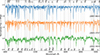 |
Fig. 1. Comparison of the normalized observed spectrum of J1022−3414 and those of two known LP 40−365 type stars from Raddi et al. (2019) retrieved from the ESO archive. The two known LP 40−365 type stars have been smoothed to the same resolution as J1022−3414 and the wavelengths are at rest. Lines of magnesium, neon, and oxygen are marked. J1022−3414 shows broader lines than the other two. |
3. Spectroscopy
The co-added spectrum has a median S/N of ∼45, enabling many individual elemental lines to be identified. Blueshifted lines of O I, Mg II, and Ne I are very clearly identified in the spectrum. Due to the lower Teff of the LP 40−365 type stars from Raddi et al. (2019), Ne I lines were visible only at the red end of the optical range, with the strongest line at 6402 Å – outside of the wavelength coverage of our spectrum. However, the presence of higher-excitation lines in our bluer spectrum reflects the higher Teff (19600 ± 700 K) of this object. We also detect many weaker lines arising from C II, O II, Mg I, AlII/III, Si II, and Ca II. The strongest and sharpest lines in the spectrum were compared with the model to infer a high barycentric RV of −390 ± 20 km s−1, again similar to the class of LP 40−365 type objects.
The spectrum was fitted using the latest version of the Koester white dwarf model atmosphere code (Koester 2010). While primarily designed for modelling white dwarfs, this LTE (local thermodynamic equilibrium) code has been successfully used in the past for modelling LP 40−365-stars (Raddi et al. 2018, 2019) and D6 stars (Hollands et al. 2025). We included all detected elements in the model calculation as listed above, but also all other elements detected in the LP 40−365-like star J1825−3757 (Raddi et al. 2019), at the same abundances relative to neon, which was the most abundant element for those stars. Approximately 25 000 lines spanning the EUV to the NIR were included in both the atmospheric structure calculations and the spectral synthesis. It was necessary for this hotter star to include as many lines as practicable, as half the flux was found to be emitted between 1500−3000 Å, and so the effect of metal line blanketing in this region, and its effect on redistributing flux to redder wavelengths, needed to be considered. Similarly to Hollands et al. (2025) who modelled a ≈16 000 K D6 star, we found that the majority of these metal lines were very narrow (with full width half maxima of the order of 0.01 Å). While these individual lines have a negligible impact on the continuum flux, their combined contribution to the emergent flux cannot be ignored, and leads to an effective lowering of the optical continuum after convolving to the instrumental resolution. For wavelengths bluer than ≈4500 Å, the continuum opacity of our models is dominated by bound-free opacities of O I, Ne I, and Mg II. These bound-free opacities, as well as those from other abundant elements in our models, were included from the Opacity Project (Cunto et al. 1993). At redder wavelengths, the continuum is instead formed from the free-free opacity of these metals. For all model calculations, fluxes were converged to 0.1% accuracy.
For the fit itself, we made Teff, log g, and number abundances of C, O, Mg, Si, and Ca (relative to Ne) free parameters, minimizing the χ2 between the data and the model (least squares fit), the latter of which was convolved to an instrumental resolution of 1.9 Å. A fixed RV of −390 km s−1 (as measured above) was applied to all models throughout. To account for the uncertain interstellar reddening and inaccuracies in flux calibration, at each step in the fit we took the ratio of the spectrum and model, fitting with a fifth-order polynomial. The model fluxes were then normalized by rescaling with this polynomial, leaving only features that varied rapidly with wavelength, i.e. absorption lines. Since aluminium has only a small number of relatively weak lines, it does not have a strong effect on the atmospheric structure. Therefore, we fitted the Al abundance independently by constructing a 1D grid of models, reducing the number of free parameters in the former least squares fit.
The best-fitting model is illustrated in Fig. 2 and the corresponding atmospheric parameters and stellar abundances are listed in Table 2. Although neon is the most abundant element by number, abundances are reported relative to oxygen, as this element was found to dominate the continuum opacity. The abundance of neon confirms the observed trend of neon-dominated atmospheres for LP 40−365 type stars, in stark contrast to D6 stars, which are carbon-dominated. Upper limits were derived for hydrogen, helium, and iron. Helium in particular was constrained better than previous studies owing to the higher temperature of this star. The upper limit of log(He/O) = − 2.8 is lower than those of LP 40−365 and J1603−6613 as studied by Raddi et al. (2019). Since the O/Ne ratio of the best-fit model is extraordinary, two models that have abundances similar to ONe-cores of ultra-massive white dwarfs were also produced. These models did not fit the data as well, but are discussed in Appendix C.
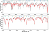 |
Fig. 2. Best-fit spectrum in the rest-frame (red) overlaid on top of the co-added FORS2 spectrum (grey). Prominent lines of oxygen (blue), neon (orange), and magnesium (green) are marked. |
Stellar atmospheric parameters and abundance ratios.
Similar to Hollands et al. (2025), the statistical uncertainties were found to be small (e.g. ∼0.01 dex for abundances), and so we estimated the uncertainties by constructing 1D grids of models for each parameter around the best-fitting values (steps of 50 K in Teff and 0.05 dex in log g and abundances). These grids were visually compared to the data to determine the uncertainties. An example of the impact of the Teff on the Mg line at 4740 Å is shown in Fig. 3. The log g has a much higher uncertainty than the one of normal white dwarfs due to the asymmetric impact on various metal lines. The Bayesian approach of Hollands et al. (2020) was used to determine the 99th percentile upper limits of log(H/O), log(He/O), and log(Fe/O). However, spectra in the wavelength range < 3800 Å will be required to better probe Fe and Ni, which are expected to form in Type Iax deflagrations.
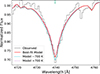 |
Fig. 3. Comparison of the best-fit model (red) and the models that have Teff of 21 300 K and 18 900 K (in purple and cyan, respectively), for a strong magnesium absorption line. |
Note that the uncertainties as described above do not account for uncertainties in atomic data, or in our models. While the best-fitting model shown in Fig. 2 shows generally good agreement, some discrepancies indicate areas for improvement. For instance, there are a few lines that are present in our spectrum that are absent in our models, most notably lines with vacuum rest wavelengths of 3939 Å and 4717 Å. For the 3939 Å line, candidate lines within 1 Å of the line centre are N III, Ti III, and Ni III. However, all candidate ions ought to have much stronger lines at other wavelengths covered by our data, which we do not observe. Similarly, for the 4717 Å line, Si III and S II are also ruled out as candidate ions. In other cases lines are correctly included in our models but fit poorly, with the 4129/4132 Å Si II doublet the most notable example. While increasing the abundance in our models will of course improve the fit to this doublet, it also introduces other Si II lines that are not observed in our data, and so the best-fitting abundance is a compromise between these considerations. This likely points to a need for improved atomic data for some weaker lines that would not normally cause problems for other types of star. It could also point to the fact that NLTE effects become more apparent at the hotter temperature of this object.
We are also limited by the number of lines we can feasibly include in our models. Each model requires several hours of computation time. When combined with the large number of necessary free parameters, the least squares fit became computationally expensive. As an experiment, we calculated a model with an order-of-magnitude more lines in the spectral synthesis, finding a visually identical spectrum in the optical (after convolving to the instrumental resolution), indicating that our reported abundances are likely to be accurate. However we also found the GALEX UV flux reduced by about 0.1 mag. This is comparable to the estimated error on the GALEX photometry (see Sect. 4), and could correspond to a 2% systematic uncertainty in Teff, which is smaller than our reported uncertainty.
Furthermore, the instrumental resolution limits the detection of any rotational broadening to v sin i > 100 km s−1. We did not find any evidence of rotational velocity greater than 100 km s−1. LP 40−365 has previously been shown to have rotational modulation in the light curve, but of the order of v sin i < 50 km s−1 (Raddi et al. 2019; Hermes et al. 2021).
Considering the fact that the atmosphere of the star is neither carbon- nor oxygen-dominated, our spectroscopic analysis does not favour a D6 or violent merger scenario. A detailed kinematic study represents the logical next step to confirm the nature of the star. However, since the kinematic analysis can be better constrained by the inter-stellar reddening and the angular diameter of the star, we first describe the photometric analysis.
4. Photometry
We used the best-fit spectral model to model the stellar energy distribution. We fit the angular diameter (Θ) and the reddening E(44 − 55) of the star using the χ2 fitting method described in Heber et al. (2018). We used the monochromatic interstellar extinction law from Fitzpatrick et al. (2019), with a fixed total-to-selective extinction parameter, R(55) = 3.02, which is an average value representative of the diffuse Galactic interstellar medium. The SED fit along with the corresponding photometry is shown in Fig. 4. We derived E(44 − 55) = 0.126 ± 0.009 mag, corresponding to E(B − V) = 0.11 ± 0.02 mag, which is only slightly higher than the line-of-sight value of E(B − V) = 0.087 mag from Schlafly & Finkbeiner (2011). The photometric parameters are shown in the lower part of Table 2.
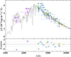 |
Fig. 4. SED of J1022−3414. Photometry was queried from DELVE DR2 (Drlica-Wagner et al. 2022), SPLUS DR4 (Herpich et al. 2024), Gaia DR3 (Gaia Collaboration 2023), SkyMapper (Onken et al. 2024), and GALEX (Martin et al. 2005). The model spectrum (in grey) is smoothed for visual clarity. The flux was multiplied with λ2 to reduce the flux steepness. |
5. Kinematic analysis
The main limitation on modelling the kinematics of these stars is the large uncertainty on their Gaia parallaxes, which limits our ability to constrain their distances. Their intrinsic absolute magnitudes are not well constrained, showing a spread of approximately MG ≈ 3.5 − 8 mag. Nevertheless, once spectroscopic information is available, kinematics provide a key discriminant between stars originating from violent mergers, double detonations, or deflagrations. In particular, the expected ejection velocities occupy distinct regions of parameter space for the different progenitor channels. We modelled the kinematics for the case of J1022−3414, using the Gaia parameters listed in Table 1. The parallax was corrected for the zero point following Lindegren et al. (2021) using the Python package GAIADR3-ZEROPOINT.
5.1. The lower limit of distance
The 2σGaia upper limit on the parallax corresponds to a lower limit on the distance of 1.8 kpc. This corresponds to a tangential velocity (Vt) of 252 km s−1. Combined with the RV, the heliocentric spatial velocity of the star would be 464 km s−1. Corrected for values of the Sun’s motion from Schönrich et al. (2010), the Galactocentric lower bound is ∼706 km s−1, suggesting that the star was boosted due to Galactic rotation. This velocity is higher than the local escape velocity, ∼550 km s−1 (Koppelman & Helmi 2021), making the star unbound. A lower limit of the absolute magnitude of the star in the GaiaG band ( ) would be 7.45 mag, close to the lower end of the observed LP 40−365 -type stars (El-Badry et al. 2023).
5.2. Distance sampling with flat magnitude prior
We used the Python package emcee (Foreman-Mackey et al. 2013) to sample the posterior distribution of the Gaia G-band absolute magnitude, MG, the mass, and the pm components of the target. Similar to El-Badry et al. (2023) we relied on the Gaia ϖ, proper motions (μα*, μδ), apparent magnitude, G, and reddening, E(B–V). We used the astrometric covariance matrix, Σobs, constructed from Gaia uncertainties and correlations. Following Hollands et al. (2025), we added spectro-photometric constraints: angular diameter, log Θ, and surface gravity, log g. To make sure that the sampling was physical, we added a mass prior: M < 1.3 M⊙, using  and
and  . The likelihood function for vector (ϖ,MG) was compared using ϖpred = 10(MG − G + 10 + AG)/5, where AG is the extinction, 2.7 × E(B − V), from Casagrande & VandenBerg (2018). We used the astrometric vector,
and the astrometric log-likelihood:
We added the predicted log g to the likelihood as
The uncertainties on Θ, and E(B − V), were added in quadrature to the likelihood for log g and ϖ, respectively.
The mass was initialized uniformly between 0.1 − 1.3 M⊙ and the upper bound of (< 1.3 M⊙) is conservative, reflecting an upper limit of remnant masses that might be left behind after deflagration of a Chandrasekhar-mass white dwarf. Work on the D6 stars (Bhat et al. 2025; Glanz et al. 2025; Bhat et al. 2026; Wong & Bildsten 2025) shows that objects less massive than 0.1 M⊙ or more massive than 0.5 M⊙ will either be too cold or too hot, respectively, compared to our star. Work on fully convective and heated C/O and O/Ne white dwarf models shows the same result, since the Kelvin-Helmholtz cooling is set by the mass and luminosity (Shen 2025). We explore this prior in Appendix B. We initialized the absolute magnitude by using a uniform distribution for MG based on the other known LP 40−365 -type stars, assuming a flat prior on MG between 0 and 15, and a positive prior on ϖ. We also applied an upper bound of 20 kpc on the derived distance, which corresponds to an upper bound of ∼2500 km s−1 on the ejection velocity of the star. 2500 km s−1 reflects a conservative bound, which is achievable only in rare cases through the violent merger scenario of Pakmor et al. (2026) or for white dwarfs more massive than 1.1 M⊙ in the D6 scenario (El-Badry et al. 2023).
The total log-posterior is then

We used 128 walkers for 10000 steps and discarded the first 4000 as burn-in. This allowed us to reach chain lengths greater than 50 auto-correlation times, which is recommended for convergence, and have enough independent samples after burn-in.
The corner plot is shown in Fig. 5 and the corresponding statistics are given in Table 3. The radius, ejection velocity, and time of flight were derived from the sampled parameters. The high correlation between the parameters is clear, with the parallax being the main source of uncertainty. The Galactocentric ejection velocity was calculated assuming a straight line path and subtracting the rotation of the Galaxy at plane crossing, similar to El-Badry et al. (2023). We assumed a circular velocity of 240 km s−1. While there seems to be a positive correlation between mass and ejection velocity, this correlation appears to be small. The uncertainty in log g shows up in the mass distribution and without any other prior is very uncertain. Higher-mass, higher-velocity stars may be produced in the double detonation mechanism, but that scenario is excluded due to the spectroscopic results, since carbon is not the dominant element.
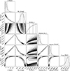 |
Fig. 5. Posterior distributions of the distance, absolute magnitude, mass, radius, ejection velocity, and midplane-crossing time. Vertical dashed lines represent 16 − 84% confidence intervals. |
Parameters sampled with emcee with mode, median, and 16−84% confidence intervals.
A flat magnitude prior (p(M) = const) implies an inverse distance prior (p(d)∝d−1). From geometric considerations it can be shown that this implies that ρ(d)∝d−3. In the case of ejected runaways, this is most likely not true. Therefore, we also tested a constant density prior that implies that p(d)∝d2, and should be valid for such runaway stars up to a distance scale proportional to their thermal times (which sets the timescale for their inflated radii when they become observable). This prior is discussed in Appendix A.
5.3. Kinematic age
We also calculated precise trajectories from the sampled distances and the measured RV as described in Irrgang et al. (2013, 2018). We used a revised version of the mass model introduced by Allen & Santillan (1991), which is called Model 1 in Irrgang et al. (2013), for the Galactic potential. We numerically integrated the equations of motion for the stars using a fourth-order Runge-Kutta solver with adaptive step size. The local standard of rest velocities (U, V, W)⊙ are (11.10 ± 1.25, 12.24 ± 2.05, 7.25 ± 0.62) km s−1, taken from Schönrich et al. (2010).
Out of the 105 computed trajectories, the star is bound for 0.005% of the simulated trajectories. Nine representative 3D trajectories, corresponding to the 68% confidence thresholds, are shown in Fig. 6. The star has a high uncertainty in the Galactic y co-ordinate stemming from the distance uncertainty but was ejected almost perpendicular to the disc. The ejection velocity of the star calculated by removing the Galactic rotation at the point of disc crossing, and assuming a 1 kpc disc scale height, lies within 608 − 1190 km s−1 (16 − 84% confidence interval). The corresponding time of flight of  Myr is in line with those of other LP 40−365 type stars.
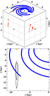 |
Fig. 6. Top panel: 3D kinematic trajectory of the star since disc ejection. Blue curves show representative spiral arms from Hou & Han (2014). The Sun is marked by the yellow circle and the Galactic centre by the black plus. Bottom panel: 2D plane-crossing contours marking regions where 68% and 95% of the trajectories intersected the Galactic plane when uncertainties were propagated. |
6. Evolutionary status and the problem with Type Iax survivors
Partial deflagrations of CO white dwarfs have previously been studied as the progenitors of Type Iax SNe (Lach et al. 2022). Hybrid CONe white dwarfs and ONe white dwarfs are other systems that have been studied (Kromer et al. 2015). However, recent observations show that the surface abundances, mainly the high neon abundances of observed surviving remnants, are incompatible with the nucleosynthesis yields of such explosions from CO white dwarfs (Raddi et al. 2019). Abundance patterns from deflagrations in ONe white dwarfs might be better suited to explain the observed spectra, which are dominated by neon and oxygen but still do not produce neon that is more abundant than oxygen. In fact, no known standard mechanism has so far been shown to produce neon that is this abundant. These stars are significantly different from the hottest D6 stars. Helium-deficient stars also include post-AGB stars called PG1159 stars. However, both D6 and PG1159 stars have high carbon and oxygen abundances and only marginal amounts of neon (Werner et al. 2024). We performed envelope calculations (the procedure is described in detail in Koester et al. 2020) by integrating the atmospheric model downwards. We found that neon is less buoyant than oxygen in the star’s outer convective zone, and therefore diffusion processes are unlikely to explain the overabundance of neon that we observe. Furthermore, the remnant masses and kicks received through these deflagration (see for example Lach et al. 2022) are too low to explain the observed velocities by at least a factor of 2 for the fastest simulated velocities.
However, heated post-explosion models can still help shed some light on the evolutionary state of these stars, especially to describe their inflated states (Zhang et al. 2019). Using the 1D stellar evolution code Modules for Experiments in Stellar Astrophysics (MESA, Paxton et al. 2011, 2013, 2015, 2018, 2019; Jermyn et al. 2023), Shen (2025) showed that the Kelvin-Helmholtz cooling of initially fully convective ONe stars could explain the inflated nature of the observed LP 40−365 type stars.
We show the Kiel diagram for the evolutionary tracks of Shen (2025) in Fig. 7. We overplot a few known LP 40−365 type stars taken from Raddi et al. (2019) and the suspected LP 40−365 type star J1240+6710 (Gänsicke et al. 2020; Kepler et al. 2016) for which a spectral analysis with a corresponding log g exists. Our object is hotter than every other known LP 40−365 type star and more inflated than all but one. The lower log g shows this to be the case. The evolutionary track of the 0.3 M⊙ model matches our observation quite well. The results of the kinematic analysis cannot be compared further due to a lack of higher-mass evolutionary models. While the ages of these models are prone to uncertainty due to starting entropy profiles (see the discussion and comparison in Bhat et al. 2026), the upper limit of a few million years matches the calculated kinematic age well (see Table 4).
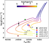 |
Fig. 7. Kiel diagram of the observed stars plotted over evolutionary tracks of ONe-dominated cooling convective balls from Shen (2025). A lower limit of 0.20 M⊙ may be established for the mass of J1022−3414 due to the observed Teff. |
Orbital parameters for J1022−3414.
The inflated nature of the star is also reflected in the colour-magnitude diagram, as is shown in Fig. 8. Overplotted are the known LP 40−365 -type stars taken from El-Badry et al. (2023), and 10000 stars within 100 pc in Gaia, showing that the star is the hottest and second most inflated LP 40−365 -type star known.
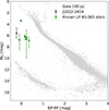 |
Fig. 8. Colour-magnitude diagram of the confirmed LP 40−365 type stars from El-Badry et al. (2023) in green. Background stars (in grey) were selected from the Gaia 100 pc sample. J1022−3414 is plotted in red with the absolute magnitude sampled using the emcee procedure described before. |
In Fig. 9 we plot the measured ejection velocities of the observed stars as a function of their mass. Along with the observations, we also plot results of 3D simulations from the works of Jordan et al. (2012) and Lach et al. (2022). While other models exist, in particular the oxygen deflagration models of Jones et al. (2016, 2019) that lead to lower-mass remnants (0.366 M⊙ at the lowest), kick velocities are not reported for them. Similarly the models of Fink et al. (2014) are not plotted due to negligible kick velocities. We also plot curves for the expectation from a simple momentum conservation argument, wherein asymmetric ejecta with an ejecta velocity, Vej, with an asymmetry factor, f, from an initial white dwarf (Mi) lead to a remnant mass, Mrem, such that the kick velocity may be written as
 (1)
(1)
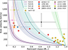 |
Fig. 9. Ejection velocities of the observed LP 40−365 type stars as a function of their derived masses. Yellow squares and red diamonds are deflagration models from Lach et al. (2022) and Jordan et al. (2012), respectively. Curves show different kick velocities from ejecta derived using Eq. (1) for different asymmetry factors. The spread for each curve was computed using ejecta velocities between 3000 − 8000 km s−1. The dashed grey line shows the maximum velocity achieved by any model so far. |
Since it is assumed that the deflagrations are Chandrasekhar-mass, we assume the initial white dwarf mass to be 1.4 M⊙. The analytical expression matches well for 1 − 5% asymmetry, which is characterized by a slightly off-centre ignition.
The simulated models so far cannot consistently produce such low-mass remnants with similar ejection velocities to those observed. Furthermore, these models have differences in their gravity solvers that rely on monopole or multipole expansion and that lead to different kick velocities. As such the higher velocities of the remnants from Jordan et al. (2012) might be a consequence of a different solver. Fink et al. (2014) pointed this out as they were unable to reproduce the kick velocities most likely because of their monopole solver. Shifting to an FFT-based solver, however, still did not significantly increase the kicks in their study.
7. Discussion
In this paper we have detailed the spectroscopic and kinematic analysis of the hottest (Teff = 19 600 ± 700 K) and second-most inflated (radius of 0.32 − 0.74 R⊙) confirmed LP 40−365 type star. The spectroscopic results show a high neon abundance, followed by oxygen, in line with previous results of LP 40−365 type stars, and different from known runaway donors of Type Ia SNe, which are carbon-dominated. A Bayesian analysis using the Gaia astrometric and photometric parameters, the spectroscopic log g, and the photometric angular diameter and reddening suggests that the star is unbound from the Milky Way and was ejected ∼2.8 Myr ago from the Galactic disc.
Taken together, the observations of all LP 40−365 stars offer a comprehensive view of this class and pose a significant challenge to existing theoretical models. The following summarises the problems.
-
The abundance issue. While the presence of heavier elements has been suggested to be a signature of Chandrasekhar-mass deflagrations, no current deflagration model is able to reproduce the neon-rich abundances of the observed stars. Models only predict carbon- or oxygen-dominated survivors. Our spectroscopic models with higher O/Ne ratios are discussed in Appendix C. The data prefers models that have a lower O/Ne ratio. This seems to be the case for all the LP 40−365 type stars whose spectra have been modelled. The influence of reaction rates on the core mass fractions of ONe white dwarfs provides an interesting avenue to study. Similar studies have found that the carbon and oxygen fractions can change significantly (up to 60%) with reaction rates for CO white dwarfs (Fields et al. 2016). Similar results have been found for the mass compositions of heavier elements for core-collapse progenitors (Fields et al. 2018). The reaction rates would need to be significantly different than what is assumed in stellar evolution codes for the abundances to be reproduced, and would therefore have massive consequences for other areas of study as well.
-
The ejection velocity issue. From observations, slightly asymmetric, off-centre ignited deflagrations that eject more than 0.9 M⊙ and lead to bound remnants less than 0.5 M⊙ are favoured. However, most models show higher remnant masses (> 0.5 M⊙) and lower kicks. The orbital velocity of massive ONe accretors at the time of Roche-lobe overflow from a He star companion should be of the order of 200 − 300 km s−1. It should be even lower for main-sequence companions. In the highly improbable case in which every deflagration gives a preferential kick in the direction of orbital motion, the minimal kick based on observed ejection velocities would have to be of the order of 400 km s−1, significantly larger than what simulations can currently produce.
-
The mass issue. Similarly to ejection velocities, most models end up creating massive survivors (> 0.5 M⊙). These are far off from the 0.1 − 0.3 M⊙ values inferred for most of the LP 40−365 -type stars. In the case of J1022−3414, the mass is not well constrained and a higher value is favoured, but so far this remains an exception.
Finally, an observational lack of fast (> 800 km s−1) He star donors (in comparison with accretors) to this channel further contributes to an already confusing picture. The unbound He-sdO US708 is the only known star of this kind (Hirsch et al. 2005; Geier et al. 2015), but is expected to be the surviving donor of a SN Ia. A fast-moving (∼600 − 800 km s−1) population of He star donors (some of which may be partially degenerate) has been predicted for Type Ia SNe (Rajamuthukumar et al. 2025). While matching the kick velocities observed for LP 40−365 type stars, they cannot explain the high observed neon abundances. This lack of observed He star donors may be alleviated slightly by a slower moving main-sequence star donor population. For now, LP 40−365 type stars present an opportunity to better understand some of the most peculiar supernovae in our Galaxy.
Acknowledgments
We thank the anonymous referee for their helpful comments. A.B. was supported by the Deutsche Forschungsgemeinschaft (DFG) through grant GE2506/18-1. Based on observations collected at the European Southern Observatory under ESO programme 115.28G1.002. We thank Abinaya Swaruba Rajamuthukumar and Evan Bauer for insightful discussions. This work made use of the following software packages: matplotlib (Hunter 2007), numpy (Harris et al. 2020), python (Van Rossum & Drake 2009), Cython (Behnel et al. 2011), emcee (Foreman-Mackey et al. 2013, 2024a), corner.py (Foreman-Mackey 2016; Foreman-Mackey et al. 2024b), and h5py (Collette 2013; Collette et al. 2023). Software citation information aggregated using https://www.tomwagg.com/software-citation-station/ (Wagg & Broekgaarden 2024; Wagg et al. 2025). This work presents results from the European Space Agency (ESA) space mission Gaia. Gaia data are being processed by the Gaia Data Processing and Analysis Consortium (DPAC). Funding for the DPAC is provided by national institutions, in particular the institutions participating in the Gaia MultiLateral Agreement (MLA). The Gaia mission website is https://www.cosmos.esa.int/gaia. The Gaia archive website is https://archives.esac.esa.int/gaia.
References
- Allen, C., & Santillan, A. 1991, Rev. Mexicana Astron. Astrofis., 22, 255 [Google Scholar]
- Arnett, W. D., Branch, D., & Wheeler, J. C. 1985, Nature, 314, 337 [Google Scholar]
- Behnel, S., Bradshaw, R., Citro, C., et al. 2011, Comput. Sci. Eng., 13, 31 [Google Scholar]
- Bhat, A., Bauer, E. B., Pakmor, R., et al. 2025, A&A, 693, A114 [NASA ADS] [CrossRef] [EDP Sciences] [Google Scholar]
- Bhat, A., Pakmor, R., Shen, K. J., Bauer, E. B., & Rajamuthukumar, A. S. 2026, A&A, 706, A375 [NASA ADS] [CrossRef] [EDP Sciences] [Google Scholar]
- Bloom, J. S., Kasen, D., Shen, K. J., et al. 2012, ApJ, 744, L17 [NASA ADS] [CrossRef] [Google Scholar]
- Boos, S. J., Townsley, D. M., Shen, K. J., Caldwell, S., & Miles, B. J. 2021, ApJ, 919, 126 [NASA ADS] [CrossRef] [Google Scholar]
- Camisassa, M. E., Althaus, L. G., Córsico, A. H., et al. 2019, A&A, 625, A87 [NASA ADS] [CrossRef] [EDP Sciences] [Google Scholar]
- Casagrande, L., & VandenBerg, D. A. 2018, MNRAS, 479, L102 [NASA ADS] [CrossRef] [Google Scholar]
- Collette, A. 2013, Python and HDF5 (O’Reilly) [Google Scholar]
- Collette, A., Kluyver, T., Caswell, T. A., et al. 2023, https://doi.org/10.5281/zenodo.7560547 [Google Scholar]
- Cunto, W., Mendoza, C., Ochsenbein, F., & Zeippen, C. J. 1993, A&A, 275, L5 [NASA ADS] [Google Scholar]
- Dan, M., Rosswog, S., Guillochon, J., & Ramirez-Ruiz, E. 2011, ApJ, 737, 89 [NASA ADS] [CrossRef] [Google Scholar]
- Dan, M., Rosswog, S., Guillochon, J., & Ramirez-Ruiz, E. 2012, MNRAS, 422, 2417 [NASA ADS] [CrossRef] [Google Scholar]
- DES Collaboration (Abbott, T. M. C., et al.) 2024, ApJ, 973, L14 [NASA ADS] [CrossRef] [Google Scholar]
- Drlica-Wagner, A., Ferguson, P. S., Adamów, M., et al. 2022, ApJS, 261, 38 [NASA ADS] [CrossRef] [Google Scholar]
- El-Badry, K., Shen, K. J., Chandra, V., et al. 2023, Open J. Astrophys., 6, 28 [CrossRef] [Google Scholar]
- Fields, C. E., Farmer, R., Petermann, I., Iliadis, C., & Timmes, F. X. 2016, ApJ, 823, 46 [CrossRef] [Google Scholar]
- Fields, C. E., Timmes, F. X., Farmer, R., et al. 2018, ApJS, 234, 19 [NASA ADS] [CrossRef] [Google Scholar]
- Fink, M., Hillebrandt, W., & Röpke, F. K. 2007, A&A, 476, 1133 [NASA ADS] [CrossRef] [EDP Sciences] [Google Scholar]
- Fink, M., Kromer, M., Seitenzahl, I. R., et al. 2014, MNRAS, 438, 1762 [NASA ADS] [CrossRef] [Google Scholar]
- Fitzpatrick, E. L., Massa, D., Gordon, K. D., Bohlin, R., & Clayton, G. C. 2019, ApJ, 886, 108 [Google Scholar]
- Foley, R. J., Challis, P. J., Chornock, R., et al. 2013, ApJ, 767, 57 [Google Scholar]
- Foreman-Mackey, D. 2016, J. Open Source Softw., 1, 24 [Google Scholar]
- Foreman-Mackey, D., Hogg, D. W., Lang, D., & Goodman, J. 2013, PASP, 125, 306 [Google Scholar]
- Foreman-Mackey, D., Farr, W. M., Archibald, A., et al. 2024a, https://doi.org/10.5281/zenodo.10996751 [Google Scholar]
- Foreman-Mackey, D., Price-Whelan, A., Vousden, W., et al. 2024b, https://doi.org/10.5281/zenodo.14209694 [Google Scholar]
- Freudling, W., Romaniello, M., Bramich, D. M., et al. 2013, A&A, 559, A96 [NASA ADS] [CrossRef] [EDP Sciences] [Google Scholar]
- Gaia Collaboration (Vallenari, A., et al.) 2023, A&A, 674, A1 [NASA ADS] [CrossRef] [EDP Sciences] [Google Scholar]
- Gänsicke, B. T., Koester, D., Raddi, R., Toloza, O., & Kepler, S. O. 2020, MNRAS, 496, 4079 [CrossRef] [Google Scholar]
- Geier, S., Fürst, F., Ziegerer, E., et al. 2015, Science, 347, 1126 [Google Scholar]
- Glanz, H., Perets, H. B., Bhat, A., & Pakmor, R. 2025, Nat. Astron., 9, 1523 [Google Scholar]
- Guillochon, J., Dan, M., Ramirez-Ruiz, E., & Rosswog, S. 2010, ApJ, 709, L64 [Google Scholar]
- Harris, C. R., Millman, K. J., van der Walt, S. J., et al. 2020, Nature, 585, 357 [NASA ADS] [CrossRef] [Google Scholar]
- Heber, U., Irrgang, A., & Schaffenroth, J. 2018, Open Astron., 27, 35 [Google Scholar]
- Hermes, J. J., Putterman, O., Hollands, M. A., et al. 2021, ApJ, 914, L3 [Google Scholar]
- Herpich, F. R., Almeida-Fernandes, F., Oliveira Schwarz, G. B., et al. 2024, A&A, 689, A249 [NASA ADS] [CrossRef] [EDP Sciences] [Google Scholar]
- Hirsch, H. A., Heber, U., O’Toole, S. J., & Bresolin, F. 2005, A&A, 444, L61 [NASA ADS] [CrossRef] [EDP Sciences] [Google Scholar]
- Hollands, M. A., Tremblay, P.-E., Gänsicke, B. T., et al. 2020, Nat. Astron., 4, 663 [CrossRef] [Google Scholar]
- Hollands, M. A., Shen, K. J., Raddi, R., et al. 2025, MNRAS, 541, 2231 [Google Scholar]
- Hou, L. G., & Han, J. L. 2014, A&A, 569, A125 [NASA ADS] [CrossRef] [EDP Sciences] [Google Scholar]
- Hunter, J. D. 2007, Comput. Sci. Eng., 9, 90 [NASA ADS] [CrossRef] [Google Scholar]
- Irrgang, A., Wilcox, B., Tucker, E., & Schiefelbein, L. 2013, A&A, 549, A137 [NASA ADS] [CrossRef] [EDP Sciences] [Google Scholar]
- Irrgang, A., Kreuzer, S., & Heber, U. 2018, A&A, 620, A48 [NASA ADS] [CrossRef] [EDP Sciences] [Google Scholar]
- Jermyn, A. S., Bauer, E. B., Schwab, J., et al. 2023, ApJS, 265, 15 [NASA ADS] [CrossRef] [Google Scholar]
- Jha, S., Branch, D., Chornock, R., et al. 2006, AJ, 132, 189 [NASA ADS] [CrossRef] [Google Scholar]
- Jones, S., Röpke, F. K., Pakmor, R., et al. 2016, A&A, 593, A72 [NASA ADS] [CrossRef] [EDP Sciences] [Google Scholar]
- Jones, S., Röpke, F. K., Fryer, C., et al. 2019, A&A, 622, A74 [NASA ADS] [CrossRef] [EDP Sciences] [Google Scholar]
- Jordan, G. C., Perets, H. B., Fisher, R. T., & van Rossum, D. R. 2012, ApJ, 761, L23 [NASA ADS] [CrossRef] [Google Scholar]
- Kelly, P. L., Fox, O. D., Filippenko, A. V., et al. 2014, ApJ, 790, 3 [NASA ADS] [CrossRef] [Google Scholar]
- Kepler, S. O., Koester, D., & Ourique, G. 2016, Science, 352, 67 [Google Scholar]
- Koester, D. 2010, Mem. Soc. Astron. Ital., 81, 921 [Google Scholar]
- Koester, D., Kepler, S. O., & Irwin, A. W. 2020, A&A, 635, A103 [NASA ADS] [CrossRef] [EDP Sciences] [Google Scholar]
- Koppelman, H. H., & Helmi, A. 2021, A&A, 649, A136 [NASA ADS] [CrossRef] [EDP Sciences] [Google Scholar]
- Kromer, M., Sim, S. A., Fink, M., et al. 2010, ApJ, 719, 1067 [Google Scholar]
- Kromer, M., Ohlmann, S. T., Pakmor, R., et al. 2015, MNRAS, 450, 3045 [NASA ADS] [CrossRef] [Google Scholar]
- Lach, F., Callan, F. P., Bubeck, D., et al. 2022, A&A, 658, A179 [NASA ADS] [CrossRef] [EDP Sciences] [Google Scholar]
- Li, W., Filippenko, A. V., Chornock, R., et al. 2003, PASP, 115, 453 [Google Scholar]
- Lindegren, L., Hernández, J., Bombrun, A., et al. 2018, A&A, 616, A2 [NASA ADS] [CrossRef] [EDP Sciences] [Google Scholar]
- Lindegren, L., Bastian, U., Biermann, M., et al. 2021, A&A, 649, A4 [EDP Sciences] [Google Scholar]
- Martin, D. C., Fanson, J., Schiminovich, D., et al. 2005, ApJ, 619, L1 [Google Scholar]
- Mehta, V., Sullivan, J., Fisher, R., et al. 2024, MNRAS, 532, 1087 [Google Scholar]
- Michaelis, A., & Perets, H. B. 2025, ArXiv e-prints [arXiv:2507.16907] [Google Scholar]
- Neunteufel, P., Kruckow, M., Geier, S., & Hamers, A. S. 2021, A&A, 646, L8 [NASA ADS] [CrossRef] [EDP Sciences] [Google Scholar]
- Nomoto, K. 1982, ApJ, 253, 798 [Google Scholar]
- Nugent, P. E., Sullivan, M., Cenko, S. B., et al. 2011, Nature, 480, 344 [NASA ADS] [CrossRef] [Google Scholar]
- Onken, C. A., Wolf, C., Bessell, M. S., et al. 2024, PASA, 41, e061 [NASA ADS] [CrossRef] [Google Scholar]
- Pakmor, R., Kromer, M., Taubenberger, S., & Springel, V. 2013, ApJ, 770, L8 [Google Scholar]
- Pakmor, R., Callan, F. P., Collins, C. E., et al. 2022, MNRAS, 517, 5260 [NASA ADS] [CrossRef] [Google Scholar]
- Pakmor, R., Shen, K. J., Bhat, A., et al. 2026, A&A, 706, A239 [NASA ADS] [CrossRef] [EDP Sciences] [Google Scholar]
- Paxton, B., Bildsten, L., Dotter, A., et al. 2011, ApJS, 192, 3 [Google Scholar]
- Paxton, B., Cantiello, M., Arras, P., et al. 2013, ApJS, 208, 4 [Google Scholar]
- Paxton, B., Marchant, P., Schwab, J., et al. 2015, ApJS, 220, 15 [Google Scholar]
- Paxton, B., Schwab, J., Bauer, E. B., et al. 2018, ApJS, 234, 34 [NASA ADS] [CrossRef] [Google Scholar]
- Paxton, B., Smolec, R., Schwab, J., et al. 2019, ApJS, 243, 10 [Google Scholar]
- Phillips, M. M., Li, W., Frieman, J. A., et al. 2007, PASP, 119, 360 [CrossRef] [Google Scholar]
- Raddi, R., Gentile Fusillo, N. P., Pala, A. F., et al. 2017, MNRAS, 472, 4173 [NASA ADS] [CrossRef] [Google Scholar]
- Raddi, R., Hollands, M. A., Koester, D., et al. 2018, ApJ, 858, 3 [NASA ADS] [CrossRef] [Google Scholar]
- Raddi, R., Hollands, M. A., Koester, D., et al. 2019, MNRAS, 489, 1489 [Google Scholar]
- Rajamuthukumar, A. S., Pakmor, R., Justham, S., Bhat, A., & Shen, K. J. 2025, A&A, submitted [arXiv:2511.11998] [Google Scholar]
- Riess, A. G., Filippenko, A. V., Challis, P., et al. 1998, AJ, 116, 1009 [Google Scholar]
- Ruiter, A. J., & Seitenzahl, I. R. 2025, A&ARv, 33, 1 [Google Scholar]
- Schlafly, E. F., & Finkbeiner, D. P. 2011, ApJ, 737, 103 [Google Scholar]
- Schönrich, R., Binney, J., & Dehnen, W. 2010, MNRAS, 403, 1829 [NASA ADS] [CrossRef] [Google Scholar]
- Shen, K. J. 2025, ApJ, 982, 6 [Google Scholar]
- Shen, K. J., Boubert, D., Gänsicke, B. T., et al. 2018a, ApJ, 865, 15 [Google Scholar]
- Shen, K. J., Kasen, D., Miles, B. J., & Townsley, D. M. 2018b, ApJ, 854, 52 [Google Scholar]
- Takaro, T., Foley, R. J., McCully, C., et al. 2020, MNRAS, 493, 986 [Google Scholar]
- Van Rossum, G., & Drake, F. L. 2009, Python 3 Reference Manual (Scotts Valley: CreateSpace) [Google Scholar]
- Vennes, S., Nemeth, P., Kawka, A., et al. 2017, Science, 357, 680 [Google Scholar]
- Wagg, T., & Broekgaarden, F. S. 2024, ArXiv e-prints [arXiv:2406.04405] [Google Scholar]
- Wagg, T., Broekgaarden, F., Van-Lane, P., Wu, K., & Gültekin, K. 2025, https://doi.org/10.5281/zenodo.17654855 [Google Scholar]
- Werner, K., Reindl, N., Rauch, T., El-Badry, K., & Bédard, A. 2024, A&A, 682, A42 [NASA ADS] [CrossRef] [EDP Sciences] [Google Scholar]
- Wong, T. L. S., & Bildsten, L. 2025, ApJ, 992, 108 [Google Scholar]
- Zhang, M., Fuller, J., Schwab, J., & Foley, R. J. 2019, ApJ, 872, 29 [Google Scholar]
Appendix A: Distance prior
The results for the distance prior are given in Table A.1. The star is farther away and has a higher predicted mass. The ejection velocity of the star increases slightly to 742 − 1477 km s−1 which is a consequence of the larger distance. The star is more inflated, with radius between 0.45 − 1.09 R⊙. With this distance prior, the star is even more of an outlier when considering theoretical models, as discussed in Sect. 7.
Parameters sampled with emcee with mode, median, and 16–84% confidence intervals.
Appendix B: Priors on mass and their influence on kinematics
The spectroscopic Teff combined with previous studies of such stars allows us to place a conservative limit on the mass of the star which is between 0.1 − 0.5 M⊙. Using this prior, we can constrain the ejection velocity to be within 585 − 976 km s−1 (68% confidence). The corresponding values are given in Table B.1 and the corner plot is shown in Fig. B.2. Since the mass is also constraining for the distance, there is only a 2 − 5% difference in the flat magnitude prior and the distance prior for this case. The updated velocity-mass diagram is shown in Fig. B.1.
Stellar parameters with mode, median, and 16−84% confidence intervals, assuming a < 0.5 M⊙ prior on mass.
The posterior distributions of our mass samples indicate that a substantial fraction of the samples accumulate near the imposed upper limits. For the prior M < 1.3 M⊙, approximately 20% of the posterior samples lie in the range 1.2 − 1.3 M⊙. Similarly, for the prior M < 0.5 M⊙, about 36% of the samples fall between 0.4 and 0.5 M⊙. This tendency toward higher masses is driven by the large uncertainties in log g and the parallax. Nevertheless, this behaviour does not affect our interpretation of the star’s ejection mechanism, as the inferred ejection velocity exceeds 600 km s−1 in all cases. A positive correlation between mass and distance is present due to the larger radii at higher masses, but this effect is weak. Consequently, both the flight time and the ejection velocity remain largely unchanged.
Appendix C: Standard O/Ne-core models
We also created models for two compositions with mass-fractions O/Ne = 0.5/0.4 and O/Ne = 0.58/0.3 to reflect two possible core compositions of ONe white dwarfs. For the first model C/Na/Mg fractions were 0.01/0.03/0.06, and heavier metals were fixed to their solar mass fractions. This first composition with O/Ne = 0.5/0.4 reflects an extreme case of composition in standard ONe white dwarfs. The latter composition of O/Ne = 0.58/0.3 is taken from the abundance of 1.23 M⊙ ONe white dwarf from Camisassa et al. (2019). The comparisons of the models to the data are shown in Fig. C.1. The χ2 of the models were 6014.43 for the best-fit neon-rich model, 6870.98 for O/Ne = 0.5/0.4, and 7948.05 for O/Ne = 0.58/0.3. This difference arises mainly due to the oxygen lines, which become a bit stronger and do not match the data as well. This can be seen for lines at 3750 Å, 4577 Å, 4772 Å, and 4980 Å. Therefore, our modelling of J1022-3414 as with the other analysed LP 40−365 type stars, supports a Ne-enhanced composition compared to evolutionary models of ONe core white dwarfs.
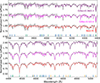 |
Fig. C.1. Comparison of three different models with different amounts of O/Ne. O/Ne ratios are given in terms of mass-fraction. The best-fit model has a nmass-fraction ratio of O/Ne of 0.28/0.67. The higher oxygen abundances lead to stronger oxygen lines such as the one at 4780 Å. |
All Tables
Parameters sampled with emcee with mode, median, and 16−84% confidence intervals.
Parameters sampled with emcee with mode, median, and 16–84% confidence intervals.
Stellar parameters with mode, median, and 16−84% confidence intervals, assuming a < 0.5 M⊙ prior on mass.
All Figures
|
Fig. 1. Comparison of the normalized observed spectrum of J1022−3414 and those of two known LP 40−365 type stars from Raddi et al. (2019) retrieved from the ESO archive. The two known LP 40−365 type stars have been smoothed to the same resolution as J1022−3414 and the wavelengths are at rest. Lines of magnesium, neon, and oxygen are marked. J1022−3414 shows broader lines than the other two. |
| In the text | |
|
Fig. 2. Best-fit spectrum in the rest-frame (red) overlaid on top of the co-added FORS2 spectrum (grey). Prominent lines of oxygen (blue), neon (orange), and magnesium (green) are marked. |
| In the text | |
|
Fig. 3. Comparison of the best-fit model (red) and the models that have Teff of 21 300 K and 18 900 K (in purple and cyan, respectively), for a strong magnesium absorption line. |
| In the text | |
|
Fig. 4. SED of J1022−3414. Photometry was queried from DELVE DR2 (Drlica-Wagner et al. 2022), SPLUS DR4 (Herpich et al. 2024), Gaia DR3 (Gaia Collaboration 2023), SkyMapper (Onken et al. 2024), and GALEX (Martin et al. 2005). The model spectrum (in grey) is smoothed for visual clarity. The flux was multiplied with λ2 to reduce the flux steepness. |
| In the text | |
|
Fig. 5. Posterior distributions of the distance, absolute magnitude, mass, radius, ejection velocity, and midplane-crossing time. Vertical dashed lines represent 16 − 84% confidence intervals. |
| In the text | |
|
Fig. 6. Top panel: 3D kinematic trajectory of the star since disc ejection. Blue curves show representative spiral arms from Hou & Han (2014). The Sun is marked by the yellow circle and the Galactic centre by the black plus. Bottom panel: 2D plane-crossing contours marking regions where 68% and 95% of the trajectories intersected the Galactic plane when uncertainties were propagated. |
| In the text | |
|
Fig. 7. Kiel diagram of the observed stars plotted over evolutionary tracks of ONe-dominated cooling convective balls from Shen (2025). A lower limit of 0.20 M⊙ may be established for the mass of J1022−3414 due to the observed Teff. |
| In the text | |
|
Fig. 8. Colour-magnitude diagram of the confirmed LP 40−365 type stars from El-Badry et al. (2023) in green. Background stars (in grey) were selected from the Gaia 100 pc sample. J1022−3414 is plotted in red with the absolute magnitude sampled using the emcee procedure described before. |
| In the text | |
|
Fig. 9. Ejection velocities of the observed LP 40−365 type stars as a function of their derived masses. Yellow squares and red diamonds are deflagration models from Lach et al. (2022) and Jordan et al. (2012), respectively. Curves show different kick velocities from ejecta derived using Eq. (1) for different asymmetry factors. The spread for each curve was computed using ejecta velocities between 3000 − 8000 km s−1. The dashed grey line shows the maximum velocity achieved by any model so far. |
| In the text | |
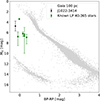 |
Fig. A.1. Same as Fig. 8 but with a distance prior. |
| In the text | |
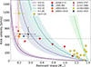 |
Fig. B.1. Same as Fig. 9 but for bounded mass priors between 0.1 − 0.5 M⊙. |
| In the text | |
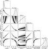 |
Fig. B.2. Same as Fig. 5 but for a bounded mass prior. |
| In the text | |
|
Fig. C.1. Comparison of three different models with different amounts of O/Ne. O/Ne ratios are given in terms of mass-fraction. The best-fit model has a nmass-fraction ratio of O/Ne of 0.28/0.67. The higher oxygen abundances lead to stronger oxygen lines such as the one at 4780 Å. |
| In the text | |
Current usage metrics show cumulative count of Article Views (full-text article views including HTML views, PDF and ePub downloads, according to the available data) and Abstracts Views on Vision4Press platform.
Data correspond to usage on the plateform after 2015. The current usage metrics is available 48-96 hours after online publication and is updated daily on week days.
Initial download of the metrics may take a while.