| Issue |
A&A
Volume 708, April 2026
|
|
|---|---|---|
| Article Number | A51 | |
| Number of page(s) | 10 | |
| Section | The Sun and the Heliosphere | |
| DOI | https://doi.org/10.1051/0004-6361/202558637 | |
| Published online | 25 March 2026 | |
Equipartition field strength on the sunspot boundary
Statistical study
1
Astronomical Institute of the Czech Academy of Sciences, Fričova 298, 25165, Ondřejov, Czech Republic
2
Institut für Sonnenphysik (KIS), Georges-Köhler-Allee 401a, 79110, Freiburg, Germany
★ Corresponding authors: This email address is being protected from spambots. You need JavaScript enabled to view it.
; This email address is being protected from spambots. You need JavaScript enabled to view it.
; This email address is being protected from spambots. You need JavaScript enabled to view it.
Received:
18
December
2025
Accepted:
17
February
2026
Abstract
Context. A recent case study of a long-lived sunspot confirmed earlier observational indications that the outer boundary of sunspots is defined by an invariant value of the magnetic field strength. This property is also found in magnetohydrodynamic sunspot simulations, which show that this invariant value corresponds to the equipartition field strength.
Aims. We investigated a large sample of sunspots throughout their evolution to statistically assess the magnetic field strength at their outer boundaries, determine whether it systematically reaches an invariant value, and evaluate possible dependences on sunspot size and evolutionary phase.
Methods. We automatically processed nearly 1000 active regions observed by the Helioseismic and Magnetic Imager on board the Solar Dynamics Observatory and identified and tracked 312 unique sunspots. The outer boundary of each sunspot was defined using a continuum-intensity threshold. For all evolutionary stages, we computed the mean magnetic field strength along this boundary and its standard deviation.
Results. Across the sample, the mean magnetic field along the boundary decreases during formation, reaches a minimum during the stable phase, and increases again during decay. For sunspots with a fully developed penumbra, this minimum is remarkably consistent, with a value of 605 ± 27 G. The standard deviation of the magnetic field exhibits a similar temporal evolution, and its minimum provides an additional diagnostic of penumbral maturity: fully developed penumbrae correspond to σB ⪅ 200 G, whereas higher values indicate either forming or decaying structures. For sunspots with fully developed penumbrae, the mean B value at their boundaries varies weakly with sunspot size; larger sunspots tend to have stronger B.
Conclusions. The results demonstrate that fully developed sunspots systematically reach an invariant magnetic field strength value, namely the equipartition field strength, at their outer boundary. The temporal evolution of the mean field and its spatial variability along the boundary provides a robust diagnostic of sunspot formation, stability, and decay.
Key words: methods: numerical / Sun: magnetic fields / Sun: photosphere / sunspots
© The Authors 2026
 Open Access article, published by EDP Sciences, under the terms of the Creative Commons Attribution License (https://creativecommons.org/licenses/by/4.0), which permits unrestricted use, distribution, and reproduction in any medium, provided the original work is properly cited.
This article is published in open access under the Subscribe to Open model. This email address is being protected from spambots. You need JavaScript enabled to view it. to support open access publication.
1. Introduction
The morphological appearance of sunspots is defined by the interaction between convective motions and the magnetic field. Sunspot umbrae are regions in which the vertical component of the magnetic field exceeds a critical value (Bvercritical) that is about 1.8 kG (Jurčák 2011; Jurčák et al. 2018; Schmassmann et al. 2018). These observational findings agree with theoretical work studying stability against overturning convection in the presence of magnetic field as Gough & Tayler (1966) derived Schwarzschild’s convective stability criterion for compressible gases, including the stabilising effect of the magnetic field. In the simplest form, the Gough & Tayler criterion for stability is given by
 (1)
(1)
where Γ1 is Schwarzschild’s first adiabatic exponent, ρ is the density, p is the pressure, and Bver is the vertical component of the magnetic field. Once Bver < Bvercritical, the overturning convection sets in and can operate, but it is still affected by the magnetic field. The Gough & Tayler criterion in sunspot simulations was investigated in detail by Schmassmann et al. (2021).
In sunspots, umbrae are surrounded by penumbrae, in which the horizontal component of the magnetic field is sufficiently strong to shape the convective cells into elongated filaments. This results in the formation of the so-called uncombed structure of the penumbra (Solanki & Montavon 1993), in which the background magnetic field of the opening sunspot magnetic funnel is mixed with horizontal fields contained within the filaments of convective origin (Tiwari et al. 2013).
Recently, Schmassmann et al. (2026) confirmed that the outer sunspot intensity boundary is well defined by a constant magnetic field strength value of about 625 G. On the other hand, from magnetohydrodynamic (MHD) sunspot simulations, Jurčák et al. (2020) found that this constant field corresponds to the equipartition field. This value is comparable to the estimates of the equipartition field strength estimated from MHD simulations of the solar photosphere (Rempel 2014). Schmassmann et al. (2026) thus confirmed two previous observational studies by Wiehr (1996) and Kálmán (2002), who found indications that the outer sunspot intensity boundary matches the iso-contour of the equipartition field strength.
From a theoretical standpoint, the equipartition field corresponds to the magnetic field strength at which the magnetic energy density equals the kinetic energy density of the moving plasma. This condition marks a natural transition between flow-dominated dynamics and regimes in which the magnetic fields play the leading role. Under this assumption, we obtain  , where ρ denotes the mass density, and v is the characteristic plasma velocity.
The theory of the equipartition field strength therefore implies that outer sunspot boundaries should correspond to Beq. Numerous studies have investigated the magnetic properties of sunspots using azimuthal averages of magnetic parameters (see e.g. Westendorp Plaza et al. 2001; Borrero et al. 2004; Bellot Rubio et al. 2004; Beck 2008; Borrero & Ichimoto 2011). These studies consistently showed that the magnetic field strength reaches its maximum in the umbral core and decreases radially outward. Depending on the data and method, the azimuthally averaged magnetic field strength at the outer sunspot boundary varies, but is typically found to be about 800 G. This value is comparable to the estimates of equipartition field strength in the solar photosphere for typical densities and velocities expected there. However, based on these studies, no direct relation between the outer sunspot boundary and Beq was established.
The analyses pointing out the similarity of B at the sunspot boundary to Beq were either based on a few vector magnetograms of a complex active region (Kálmán 2002) or on a long time series of a stable simple sunspot (Schmassmann et al. 2026). We note that Wiehr (1996) inferred on Beq using spectroscopic data alone, without performing any inversion. Therefore, it is necessary to confirm these previous observational findings using a statistical approach. This is now feasible based on the extensive archives of consistent space-based observations.
The source code we used in this work is publicly available in the GitHub repository solar-feature-contour-tracking1, released under the MIT license. This ensures full reproducibility of the data processing and statistical analysis described in this study.
2. Data selection and processing
We analysed a large set of solar active regions using data from the Helioseismic and Magnetic Imager (HMI; Scherrer et al. 2012; Schou et al. 2012) on board the Solar Dynamics Observatory (SDO; Pesnell et al. 2012). Our dataset includes all HMI Active Region Patches (HARPs) with IDs between 1 and 1500, yielding 837 time series, supplemented by additional previously collected datasets. In total, we gathered 974 candidate regions, encompassing a broad range of sunspot and pore activity. For each region, we used the HMI observables of the continuum intensity Ic and the magnetic field strength B.
The HMI observes the Fe I 617.3 nm photospheric spectral line, sampling it at six wavelength positions across the line profile with an effective spectral resolution of approximately 76 mÅ. The magnetic field strength B used in this study corresponds to the total field inferred from these filtergram measurements through the Very Fast Inversion of the Stokes Vector (VFISV), a Milne–Edington inversion code (Borrero et al. 2011). This inversion yields a magnetic field strength representative of the formation region in which the line is most sensitive.
The continuum intensity was corrected for limb darkening by applying the fifth-order polynomial in the cosine of the heliocentric angle μ using coefficients published by Pierce & Slaughter (1977, Table IV, wavelength 660.4 nm). After correction, the intensity was normalised by the median intensity of the quiet Sun, defined as the intensities outside magnetically active regions (i.e. B < 500 G) and within the range 60–95% of the maximum continuum intensity. This avoids contamination by bright points or low-contrast network features.
To enhance the spatial resolution and remove instrumental degradation, the processed observations were passed through the deep-learning-based deconvolution algorithm developed by Korda et al. (2025). This model incorporates the precise HMI point-spread function and realistic noise synthesis, restoring the image quality to a level comparable with that of Hinode’s Solar Optical Telescope Spectro-Polarimeter (SOT-SP; Tsuneta et al. 2008; Lites et al. 2013). Figure 1 illustrates the improvement, showing the original HMI continuum intensity alongside the corresponding deconvolved output produced by the neural network. The subsequent identification, tracking, classification, and analysis of sunspots and magnetic structures were carried out using these deconvolved observations. All datasets were analysed at a uniform temporal cadence of one hour.
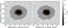 |
Fig. 1. Comparison of the original HMI continuum intensity (left) and its deconvolved version (right) for NOAA AR 11084 (HARP 71 dataset), observed on 2010 July 2 at 04:00:00 UT. The red and blue contours correspond to 0.5 and 0.9 of the original continuum intensity, respectively, and the dashed yellow and green contours indicate the same levels in the deconvolved image. The colour bars are identical in the two panels. |
2.1. Initial detection and sunspot definition
We detected the sunspots on the enhanced continuum-intensity maps produced by the neural network deconvolution model. These maps, derived from HMI observables corrected for limb darkening, allowed us to identify the fine structure in active regions more accurately.
Two fixed intensity thresholds were used to delineate dark solar features: regions with 0.5 < Ic/IQSc ≤ 0.9 were classified as penumbrae, and regions with Ic/IQSc ≤ 0.5 were identified as umbrae. To eliminate spurious or transient features, only regions with a minimum area of about 0.25 Mm2 and a minimum lifetime of 3 hours were retained. This ensured that only well-defined persistently trackable features were included in the analysis.
All regions meeting these criteria were stored, including small pores and irregular fragments, to enable future studies beyond the current scope. For this work, we exclusively focused on sunspots, which are defined as contiguous penumbral structures that may enclose no or several umbral cores. The defining boundary of a sunspot was taken to be the outer penumbral contour. Bright structures enclosed within this boundary, such as light bridges or trapped granulation, were considered part of the penumbra. Each detected sunspot was assigned a unique identifier and tracked consistently throughout its observed evolution.
This definition allowed us to unambiguously separate umbral and penumbral areas, even in morphologically complex or fragmented regions. It also enabled a consistent statistical treatment throughout the sunspot lifetime.
2.2. Sunspot filtering and phase segmentation
We applied additional filters to the full set of detected and tracked sunspot candidates to select only once-mature and well-defined sunspots for analysis. Specifically, a region was retained when it satisfied both of the following criteria: (1) The umbra persisted for at least 30 hours, ensuring that short-lived or marginal features were excluded. (2) The penumbral area exceeded about 250 Mm2 (sunspot diameter about 27″) in at least one observation during its evolution, filtering out pores and fragmentary structures. For comparison, the penumbral area shown in Fig. 1 equals 351 Mm2. When a sunspot temporarily split into multiple parts and then re-formed, the fragments were considered part of the same evolving feature as long as the time gap between disappearance and reappearance was shorter than 3 hours. When the gap exceeded this threshold, the reappearing feature was assigned a new identifier. This criterion helped us to maintain continuity in the presence of transient segmentation events while ensuring that truly distinct features were treated separately. To avoid projection effects, sunspot observations at μ < 0.4 (i.e. closer than ≈24° to the limb) were discarded from the further analysis. After we applied these filters, the final dataset comprised 312 unique sunspots tracked across a total of 43 190 frames.
To segment the temporal evolution of each sunspot into formation, stable, and decaying phases, we fitted a piecewise linear model to the time series of the total magnetic flux, normalised by its maximum value. The model complexity was increased gradually by allowing an increasing number of linear segments, starting from a single-segment base model. At each step, a candidate model with m segments was compared to the previously accepted model with n segments and was only accepted when its mean squared error was reduced by a fraction  or more relative to the most recent accepted model. The models were tested sequentially up to a maximum of ten segments, with the constraint m ≤ n + 5. The relaxed acceptance criterion for additional segments allows the algorithm to capture more complex temporal behaviour, such as multiple magnetic merging events, without immediately favouring overfitted solutions. When none of the tested candidates met the criterion, the previously accepted model was retained as optimal. On average, 2.8 segments were sufficient to capture the evolutionary trend.
Each fitted segment was then classified according to its slope k, using an empirically determined threshold of |k|≤0.00225 h−1 to define a stable phase. Segments with k > 0.00225 h−1 were classified as formation, while those with k < −0.00225 h−1 were classified as decaying. Segments shorter than 3 hours were ignored to avoid fitting noise or short-term artefacts due to detection uncertainties.
3. Results and discussion
For every sunspot and at every time step, we extracted the contour corresponding to the quiet-Sun penumbra intensity threshold (Ic/IQSc = 0.9) and evaluated the mean magnetic field strength ⟨B⟩ along this boundary. Each contour therefore provides one measurement of the penumbral boundary field. To ensure a consistent comparison across the solar disc, we applied the foreshortening correction of the pixel area and point-density correction using
 (2)
(2)
where i indexes the sampled points along a given contour, each associated with a magnetic field value Bi, dsi is the arc-length element corresponding to the spacing between neighbouring sampled points along the contour, and μi is the cosine of the heliocentric angle at the position of point i. The contour points were sampled using linear interpolation of the underlying observables, with a maximum point spacing of 0.5 px along the contour. This procedure ensured a faithful representation of the contour geometry and sufficient point density to accurately compute the mean magnetic field along the boundary.
3.1. Statistical properties of the penumbral boundary field
From the time series of 312 sunspots, we obtained 43 190 individual quiet-Sun penumbra boundary measurements, spanning the three evolutionary phases (forming, stable, and decaying). This large statistical sample allowed us to quantify not only the typical magnetic field strength at the penumbral boundary, but also the evolution of its distribution throughout the sunspot lifetime.
3.1.1. Boundary magnetic field distribution
The distributions of the mean magnetic field strength ⟨B⟩ on the penumbral boundary (see Fig. 2) rise steeply towards their modal values, followed by a comparatively slow decline. This behaviour is observed in all evolutionary phases.
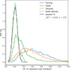 |
Fig. 2. Histograms of ⟨B⟩ for the three evolutionary phases, together with a reference histogram constructed from stable-phase observations whose boundary σB is below 130 G. A Gaussian fit to this high-stability subset provides an estimate of the magnetic field strength outlining the sunspot outer boundary. |
During the fast forming phase (18% of the contours), many penumbrae are incomplete or irregular. Local variations along the contour, caused by incomplete or merging penumbral segments, broaden the ⟨B⟩ distribution. In addition, parts of the Ic/IQSc = 0.9 contour may lie close to the umbra, sample intrinsically stronger fields, and produce a high-field tail.
During the stable phase (41% of the contours), penumbrae are typically clearly separated from the umbra and are largely uniform, resulting in a relatively narrow ⟨B⟩ distribution. Nonetheless, a modest high-field tail persists, arising from quasi-stable sunspots or partially developed penumbrae, where parts of the Ic/IQSc = 0.9 contour still sample stronger fields near the umbra. Despite these occasional high-field excursions, the bulk of the measurements is concentrated around ⟨B⟩mode ≈ 629 G, providing a direct indication of an invariant field around stable sunspots. We note that the ⟨B⟩mode agrees very well with the recent result of Schmassmann et al. (2026).
To obtain a clean estimate of the invariant field around sunspots with fully developed penumbrae, we further filtered the dataset of stable sunspots by a standard deviation σB < 130 G along a given contour. We empirically found that this threshold filters boundaries along sunspots with fully developed penumbrae. The corresponding histogram (see Fig. 2) exhibits a sharply peaked distribution, and a Gaussian fit to this subset yields our best estimate of the magnetic field strength outlining the sunspot outer boundary ⟨B⟩inv ≈ 605 ± 27 G. The extended high-field tail seen in the full distributions arises primarily from penumbrae that are not yet fully formed, where parts of the quiet-Sun penumbra boundary lie close to the umbral boundary and thus sample intrinsically stronger fields.
During the decay phase (41% of the contours), penumbrae are initially well developed and clearly separated from the umbra. As the phase progresses and the sunspot gradually loses structure, the boundary becomes increasingly irregular, producing larger local variations along the contour that broaden the ⟨B⟩ distribution. In addition, in regions in which the penumbra is absent or has partially disappeared, the Ic/IQSc = 0.9 contour samples intrinsically stronger fields closer to the sunspot centre, generating an extended high-field tail.
3.1.2. Boundary magnetic field evolution
Figure 3 shows the time series of individual ⟨B⟩ measurements for each sunspot along with the median value. To facilitate comparison among sunspots, the durations of each evolutionary phase were normalised. During the forming phase, the individual ⟨B⟩ measurements exhibit large scatter, reflecting the irregular and incomplete penumbrae discussed above. Despite this variability, the median clearly decreases over time, indicating that the penumbral boundary is moving away from the umbra and the field strength is converging towards a more stable value. The standard deviation, σB, similarly decreases throughout the forming phase, consistent with the progressive reduction of gaps and irregularities in the penumbra and the general homogenisation of the boundary.
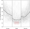 |
Fig. 3. Time series of individual ⟨B⟩ measurements for the three evolutionary phases. The thick black curve shows the phase-wise median. The solid and dashed red lines indicate the peak and standard deviation of the Gaussian fit to the high-stability subset, respectively (black curve in Fig. 2). The vertical black lines separate different phases. |
For the stable phase, the temporal median ⟨B⟩med remains approximately constant (694 ± 15 G), with only a slight decrease near the phase midpoint, indicating a well-defined and persistent field along the penumbral boundary. The standard deviation declines steeply at the start of the phase and increases gradually towards its end, likely affected by the limitations of the phase-detection algorithm at the boundaries. In the central portion of the stable phase, however, the standard deviation is less than one-third of that observed at the end of forming or the beginning of decay, demonstrating the relative uniformity and stability of the penumbral boundary in long-lived sunspots, where the field is concentrated around the invariant value.
In the decay phase, the behaviour is analogous, but with opposite trends to those in the forming phase. The phase begins with a relatively low ⟨B⟩med ≈ 780 G along the penumbral boundary, essentially the same value observed at the end of the forming phase, ⟨B⟩med ≈ 794 G, suggesting that despite the large scatter, the average penumbral boundary field exhibits similar properties at the transitions between evolutionary phases. As the decaying phase progresses, ⟨B⟩ increases gradually before culminating in a rapid rise and the development of a broad distribution towards the end of the phase. The standard deviation grows sharply in the final part of the decay, reflecting the enhanced structural irregularity and the partial disappearance of penumbral regions.
3.2. Boundary magnetic field versus sunspot size
To examine whether the boundary field depends on the sunspot size, we analysed the relation between the sunspot area and the mean magnetic field strength ⟨B⟩ measured along the Ic/IQSc = 0.9 for sunspots with fully developed penumbrae (σB < 130 G). The probability density distribution of sunspot area versus ⟨B⟩ (see Fig. 4) reveals a marginal trend: larger sunspots tend to exhibit slightly stronger boundary fields. A linear fit to the distribution yields a slope of ≈0.09 G Mm−2, implying that the average boundary field increases from roughly 570 G for small sunspots to about 650 G for the largest ones in our sample. We note that the sample of sunspots we studied is mostly populated by sunspots with areas of about 500 Mm2, while smaller and larger sunspots are observed, but there are only a few of them. The Pearson correlation coefficient between area and ⟨B⟩ is moderate, ≈0.73, indicating that the sunspot size accounts for a part, but not for all, of the observed variability in the boundary field strength. Overall, the boundary field is remarkably stable across the full range of sunspot sizes, with only a weak systematic dependence on area.
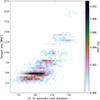 |
Fig. 4. Probability density distribution of the sunspot area and mean magnetic field strength ⟨B⟩ measured along the Ic/IQSc = 0.9 boundary for sunspots with fully developed penumbrae. |
However, from a theoretical point of view, the value should not depend on the sunspot size, as the kinetic energy density of the granulation should be the same around both large and small sunspots. To investigate the cause of the observed dependence, we examined the mean magnetic field inclination at the sunspot boundaries (not shown), and it shows no dependence on the sunspot area.
A possible source of the dependence might be a difference in stray-light contamination between large and small sunspots. However, García-Rivas et al. (2024) showed that HMI data appear to be affected by stray light only for relatively small structures that have already lost their penumbrae. Moreover, the convolutional neural network (CNN) code we applied to enhance the analysed data further reduces the role of stray light.
The measured magnetic field corresponds to photospheric heights at which the inverted line is most sensitive, well above the continuum formation height. On the other hand, the kinetic forces that disrupt the magnetic trunk of the sunspot and cause the sharp outer edge of the penumbra act below the visible solar surface. We can speculate that there might be a different gradient of the magnetic field with height between large and small sunspots that would result in the observed dependence. However, measurements of the magnetic field gradient with height are extremely complicated in the penumbra, and different studies produced different results (see the review by Balthasar 2018). We are not aware of any study showing a dependence of the magnetic field gradient on height for sunspots of different sizes.
A possible way to assess the role of the vertical gradient of the magnetic field is to repeat this analysis using spectral lines that form deeper in the photosphere, such as the Fe I lines around 1.5 μm. These lines form closer to the depths where kinetic forces disrupt the magnetic trunk of a sunspot. If the dependence of B on sunspot size were found to be weaker in this case, it would suggest that the observed trend is indeed caused by differences in the magnetic field gradient with height among sunspots of different sizes. However, we note that no space-based observations are currently available for these spectral lines, and ground-based measurements are difficult to exploit because the seeing conditions vary (as shown by Lindner et al. 2020, umbra–penumbra boundaries).
3.3. Case studies of the boundary field evolution
To complement the statistical analysis, we now examine the temporal evolution of a small set of representative sunspots. These case studies, selected to span different sizes, morphologies, and evolutionary behaviours, serve to illustrate specific features of the sunspot evolution that underlie the trends identified in the statistical sample. By following each sunspot through its forming, stable, and decaying phases, we highlight how variations in the structure and completeness of the penumbra manifest in the measured boundary field ⟨B⟩, and how the characteristic signatures of each phase appear in individual examples.
Throughout this section, active regions are identified using the numbering scheme assigned by the National Oceanic and Atmospheric Administration (NOAA). They are hereafter referred to as NOAA Active Regions (ARs).
3.3.1. NOAA Active Region 11250
We begin with sunspot NOAA AR 11250 (HARP 712 dataset), which exhibits all evolutionary phases and displays the characteristic behaviour identified in the statistical analysis. Our tracking algorithm identified the coherent magnetic structure after roughly 10 hours in which the small magnetic elements coalesced. The penumbra became fully fledged about 15 hours after the initial detection. This was followed by approximately 130 hours of stability, after which the sunspot entered a slow decay that continued until its disappearance beyond the west limb.
Figure 5 shows the temporal evolution of ⟨B⟩ and the boundary field standard deviation, together with selected intensity snapshots taken near the midpoint of each evolutionary phase. We note that the beginning of the stable phase was slightly misidentified by the algorithm; visual inspection indicates that the penumbra formation continued for an additional ≈30 hours. During the forming phase, ⟨B⟩ decreased steeply as the penumbra developed and an increasing portion of the intensity boundary was co-spatial with the outer penumbral boundary, while σB simultaneously dropped as irregular fragments merged into a coherent boundary.
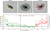 |
Fig. 5. Temporal evolution of sunspot NOAA AR 11250 (HARP 712 dataset). Top: Snapshots of the continuum intensity selected near the midpoint of each evolutionary phase with Ic/IQSc = 0.9 contours. Bottom: Time series of the mean magnetic field strength ⟨B⟩ (solid line) and the field standard deviation (dotted line). The phase is indicated by the line colours. The sunspot exhibits a clear forming, stable, and decaying phases with ⟨B⟩ approaching the invariant value (dashed black line) during the fully developed stable interval. The vertical dashed black lines mark the times corresponding to the snapshots shown in the top row. |
The stable phase exhibits an almost constant ⟨B⟩ = 622 ± 29 G. Over time, the standard deviation gradually decreased as the penumbra completed its development; initially, it was not fully developed around the ends of light bridges that separated the umbral cores. A fully developed penumbra was reached between approximately 91 and 135 hours after initial detection. Within this interval, the boundary magnetic field, ⟨B⟩ = 602 ± 22 G, agreed very well with the estimated invariant field ⟨B⟩inv.
In the decaying phase, the sunspot began to lose magnetic fragments and the boundary became increasingly irregular, leading to a sharp rise in σB. As penumbral gaps appeared, the Ic/IQSc = 0.9 boundary locally sampled stronger fields closer to the umbra, which further increased both σB and ⟨B⟩ towards the end of the time series.
To further illustrate the relation between the intensity-defined boundary and the invariant field strength, Fig. 6 shows additional snapshots with the B = ⟨B⟩inv ≈ 605 G contour overplotted. These examples confirm that the magnetic contour tracks the penumbral boundary accurately during the stable phase, whereas during formation and decay, it lies partially outside the intensity boundary, especially in regions in which the penumbra is not yet fully developed or becomes fragmented.
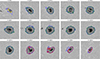 |
Fig. 6. Evolution of sunspot NOAA AR 11250 (HARP 712 dataset). Snapshots of the continuum intensity, selected at equidistant time intervals, are shown spanning the sunspot evolutionary phases. The overplotted blue contours indicate the magnetic field strength B = ⟨B⟩inv ≈ 605 G. The sunspot phases are colour-coded as in Fig. 5, and the time shown above each panel indicates the elapsed time since the first detection. |
3.3.2. NOAA Active Region 11381
Next, we considered sunspot NOAA AR 11381 (HARP 1210 dataset), which exhibits an irregular penumbra throughout its lifetime. This example is a quasi-stable sunspot with all three evolutionary phases present, each lasting roughly 50 hours. The time evolutions of ⟨B⟩ and σB are shown in Fig. 7.
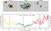 |
Fig. 7. Same as Fig. 5, but for sunspot NOAA AR 11381 (HARP 1210 dataset). The sunspot displays a quasi-stable phase with highly irregular penumbral structure despite an approximately constant total magnetic flux. |
The forming phase followed a pattern broadly similar to the representative stable sunspot: both ⟨B⟩ and σB declined gradually as penumbral segments merged and the boundary became increasingly coherent. The formation is detected approximately 2 hours after the first small magnetic elements appeared in the region.
The interval identified as the stable phase, however, is qualitatively different from that of a canonical stable sunspot. Although the total magnetic flux remains approximately constant (the criterion used for phase identification), the penumbra is highly non-uniform. At various times, granulation intruded deeply into the penumbral ring, producing large-scale intrusions, while in other locations, penumbral filaments extended outward to form elongated protrusions. The umbra was frequently split into multiple fragments, and sizeable sections of the Ic/IQSc = 0.9 contour lie close to the umbra boundary. Consequently, the boundary geometry remained highly dynamic despite the globally steady magnetic flux. We therefore refer to this interval as a quasi-stable phase: the total flux was stable, but the boundary geometry and the local field sampled by the contour varied continuously.
The decaying phase is characterised by a progressive loss of penumbral structure and increasingly frequent gaps along the boundary. Both ⟨B⟩ and σB rose as the Ic/IQSc = 0.9 contour began to sample stronger magnetic fields closer to the residual umbra. In the final stage, the sunspot became pore-like, and ⟨B⟩ along the contour fluctuated strongly.
The evolution of the B = ⟨B⟩inv ≈ 605 G contour is shown in Fig. 8. During the forming phase, the contour of the invariant field did not align with the Ic/IQSc = 0.9 boundary and lay partly outside it, reflecting the incomplete and spatially fragmented nature of the developing penumbra. Throughout the quasi-stable phase, the contour intersected the intensity boundary in multiple locations: in regions in which the penumbra was underdeveloped or temporarily disrupted, the ⟨B⟩inv ≈ 605 G contour lay outside the Ic/IQSc = 0.9 boundary, while around long extensions of penumbral filaments into quiet-Sun regions, it lay inside it. In the decaying phase, as penumbral gaps appear and the boundary became increasingly irregular, the magnetic field contour was frequently located outside the Ic/IQSc = 0.9 boundary, as the latter samples stronger fields closer to the remnant umbra. This behaviour is consistent with the strong spatial variability of ⟨B⟩ and σB measured along the boundary in this example.
3.3.3. NOAA Active Region 11084
Finally, we examined NOAA AR 11084 (HARP 71 dataset), an exceptionally stable sunspot. The sunspot appeared to be already fully developed near the east limb and maintained an essentially unchanged structure until it disappeared behind the west limb. Consequently, only a single, long-lived stable phase was present.
The temporal evolutions of ⟨B⟩ and σB are shown in Fig. 9. At the beginning of the observation, both quantities were slightly above the invariant field, with ⟨B⟩ ≈ 650 G and a comparatively large standard deviation σB ≈ 180 G. This slightly elevated scatter results from minor boundary irregularities, as small-scale faculae locally perturb the Ic/IQSc = 0.9 contour during the first hours of the time series.
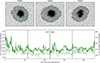 |
Fig. 9. Same as Fig. 5, but for sunspot NOAA AR 11084 (HARP 71 dataset). The sunspot remains stable over the full ≈200-hour interval, with ⟨B⟩ staying nearly constant at a value consistent with ⟨B⟩inv. |
Both quantities then quickly converged towards stable values: σB declined below 150 G, while ⟨B⟩ settled at 613 ± 16 G, a value fully consistent with ⟨B⟩inv, and remained nearly constant for the entire ≈200-hour interval. This sustained stability highlights the robustness of the penumbral boundary in this fully developed sunspot. Notably, the asymptotic value of ⟨B⟩ is essentially equal to the estimated invariant field, reinforcing the interpretation that mature, long-lived sunspots maintain a well-defined and physically meaningful boundary field strength, in agreement with Schmassmann et al. (2026).
Near the western limb, σB increased only very weakly. This indicates that the applied foreshortening and point-density corrections effectively minimise geometric effects related to projection and line-of-sight sampling. Residual variations can still be attributed to the fact that at large heliocentric angles, the contour is distorted and the line of sight samples slightly different atmospheric heights with varying magnetic structure. However, these effects introduce only a minor additional scatter in ⟨B⟩ and σB.
In this example, the Ic/IQSc = 0.9 boundary closely followed the invariant magnetic field contour, B = ⟨B⟩inv ≈ 605 G (see Fig. 10). For nearly the entire observation, the two contours overlapped almost perfectly, reflecting the remarkable stability of the magnetic and intensity boundaries. A significant deviation occurred only at the very beginning of the sequence, where small faculae temporarily interrupted the match between the contours. This same region corresponds to the elevated values of σB seen at the start of the temporal evolution in Fig. 9, as the Ic/IQSc = 0.9 boundary locally samples stronger, umbra-adjacent fields.
4. Summary and conclusions
We have systematically analysed the evolution of the sunspot outer boundary, defined by Ic/IQSc = 0.9, for 312 sunspots across 43 190 individual SDO/HMI observations, processed with our deconvolution and super-resolution pipeline (Korda et al. 2025). We used the time evolution of the magnetic flux within individual sunspots to segment it into formation, stable, and decaying phases, and we characterised the temporal evolutions of the mean magnetic field strength, ⟨B⟩, and field spatial variability, σB, along the penumbral intensity boundary.
Our results demonstrate a clear and consistent pattern across the sunspot sample. During the formation phase, the mean magnetic field along the boundary decreases, reaching a minimum that is maintained during the stable phase. For mature sunspots with fully fledged penumbra, statistically defined as σB < 130 G, this minimum corresponds to an invariant field strength ⟨B⟩inv = 605 ± 27 G, representing the typical boundary field across the full range of sunspot sizes. The mean boundary field slightly increases systematically with sunspot area, approximately 0.09 G Mm−2, rising from ≈570 G for small sunspots to ≈650 G for the largest in our sample, confirming that the boundary field is largely invariant. In the decaying phase, ⟨B⟩ increases again as penumbral structures gradually disappear. The standard deviation of the magnetic field along the boundary, σB, exhibits a similar temporal evolution, with its minimum coinciding with the presence of a fully developed penumbra. We note that the inverse evolution of ⟨B⟩ during the formation and decaying phases suggests a mirrored magnetic field evolution at the sunspot boundary.
The statistical trends were further supported by detailed case studies of representative sunspots. These examples illustrate the full temporal evolution of ⟨B⟩ and σB along individual penumbral boundaries, confirming that the patterns observed in the large dataset are representative of real sunspot behaviour. In particular, the cases highlight the characteristic decrease of ⟨B⟩ and σB during formation, their sustained low values during the stable phase, and the increase of both quantities during decay. For quasi-stable sunspots, the minimum ⟨B⟩ is 100–200 G higher than the invariant field strength found in fully developed and morphologically stable sunspots.
Additionally, we compared the Ic/IQSc = 0.9 intensity boundary with the contour corresponding to the invariant magnetic field, B = ⟨B⟩inv. For fully developed sunspots, the two contours closely coincide for most of the stable phase, with only minor deviations in regions of not yet fully developed penumbra. During the forming and decaying phases, the contours also align well in regions where the penumbra is already developed. This agreement confirms that the intensity-defined boundary reliably traces the physically relevant invariant field at the penumbral edge.
Together, these results provide strong statistical evidence that fully developed sunspots systematically attain an invariant magnetic field strength at their outer penumbral boundary. In agreement with earlier case studies (Schmassmann et al. 2026) and radiative MHD simulations (Jurčák et al. 2020), we identify this invariant value with the equipartition magnetic field strength. Our analysis further supports the interpretation proposed by Schmassmann et al. (2026), who associated the equipartition field with the surface manifestation of the underlying sunspot magnetopause, marking the transition where magnetic fields cease to dominate convective motions.
The statistical behaviour observed during the formation and decay phases in which areas are found where the intensity and the equipartition boundaries detach from each other is consistent with the existence of a distinct magneto-convective regime that differs from the penumbra and from regular quiet-Sun granulation and is characterised by granular convection coexisting with super-equipartition magnetic fields. In this regime, the magnetic field remains sufficiently strong to dominate convection, but it lacks the horizontal component required to sustain filamented penumbral magneto-convection. This naturally explains the observed decoupling between intensity-defined and magnetically defined boundaries in forming and decaying sunspots.
The statistical analysis further demonstrated that the tendency of the outer penumbral boundary to converge towards the equipartition field strength is a local property of the boundary itself and not a consequence of global sunspot or solar conditions. The boundary field reaches equipartition independently of sunspot size, total magnetic flux, or evolutionary stage, indicating that the outer penumbral edge is governed by a local magneto-convective balance. This establishes the outer boundary as a physically defined interface that limits the lateral extent of penumbral magneto-convection and acts as the primary control surface for penumbral stability and evolution.
Taken together, the radiative MHD simulations and the statistical evidence presented here suggest that sunspot evolution involves transitions between four distinct magneto-convective regimes. These include suppressed umbral convection (umbrae), penumbral magneto-convection (penumbrae), normal granular convection in sub-equipartition fields (quiet-Sun granulation), and a super-equipartition granular regime that occurs predominantly during sunspot formation and decay.
In summary, the invariant magnetic field strength at the sunspot boundary emerges as a fundamental physical property of mature sunspots, governed by the balance between magnetic and convective energy densities. The evolution of the mean boundary field strength and its spatial variability provides a quantitative framework for characterising sunspot formation, stability, and decay, and it places the concept of an equipartition-defined outer boundary within a broader classification of magneto-convective regimes.
Acknowledgments
This work was supported by the Czech-German common grant, funded by the Czech Science Foundation under the project 23-07633K and by the Deutsche Forschungsgemeinschaft under the project BE 5771/3-1 (eBer-23-13412), and the institutional support ASU:67985815 of the Czech Academy of Sciences. This research has made use of NASA’s Astrophysics Data System Bibliographic Services.
References
- Balthasar, H. 2018, Sol. Phys., 293, 120 [NASA ADS] [CrossRef] [Google Scholar]
- Beck, C. 2008, A&A, 480, 825 [NASA ADS] [CrossRef] [EDP Sciences] [Google Scholar]
- Bellot Rubio, L. R., Balthasar, H., & Collados, M. 2004, A&A, 427, 319 [NASA ADS] [CrossRef] [EDP Sciences] [Google Scholar]
- Borrero, J. M., & Ichimoto, K. 2011, Liv. Rev. Sol. Phys., 8, 4 [Google Scholar]
- Borrero, J. M., Solanki, S. K., Bellot Rubio, L. R., Lagg, A., & Mathew, S. K. 2004, A&A, 422, 1093 [NASA ADS] [CrossRef] [EDP Sciences] [Google Scholar]
- Borrero, J. M., Tomczyk, S., Kubo, M., et al. 2011, Sol. Phys., 273, 267 [Google Scholar]
- García-Rivas, M., Jurčák, J., & Bello González, N. 2024, A&A, 689, A160 [NASA ADS] [CrossRef] [EDP Sciences] [Google Scholar]
- Gough, D. O., & Tayler, R. J. 1966, MNRAS, 133, 85 [Google Scholar]
- Jurčák, J. 2011, A&A, 531, A118 [NASA ADS] [CrossRef] [EDP Sciences] [Google Scholar]
- Jurčák, J., Rezaei, R., González, N. B., Schlichenmaier, R., & Vomlel, J. 2018, A&A, 611, L4 [NASA ADS] [CrossRef] [EDP Sciences] [Google Scholar]
- Jurčák, J., Schmassmann, M., Rempel, M., Bello González, N., & Schlichenmaier, R. 2020, A&A, 638, A28 [NASA ADS] [CrossRef] [EDP Sciences] [Google Scholar]
- Kálmán, B. 2002, Sol. Phys., 209, 109 [Google Scholar]
- Korda, D., Jurčák, J., Švanda, M., & Bello González, N. 2025, A&A, 697, A28 [NASA ADS] [CrossRef] [EDP Sciences] [Google Scholar]
- Lindner, P., Schlichenmaier, R., & Bello González, N. 2020, A&A, 638, A25 [NASA ADS] [CrossRef] [EDP Sciences] [Google Scholar]
- Lites, B. W., Akin, D. L., Card, G., et al. 2013, Sol. Phys., 283, 579 [NASA ADS] [CrossRef] [Google Scholar]
- Pesnell, W. D., Thompson, B. J., & Chamberlin, P. C. 2012, Sol. Phys., 275, 3 [Google Scholar]
- Pierce, A. K., & Slaughter, C. D. 1977, Sol. Phys., 51, 25 [NASA ADS] [CrossRef] [Google Scholar]
- Rempel, M. 2014, ApJ, 789, 132 [Google Scholar]
- Scherrer, P. H., Schou, J., Bush, R. I., et al. 2012, Sol. Phys., 275, 207 [Google Scholar]
- Schmassmann, M., Schlichenmaier, R., & Bello González, N. 2018, A&A, 620, A104 [NASA ADS] [CrossRef] [EDP Sciences] [Google Scholar]
- Schmassmann, M., Rempel, M., Bello González, N., Schlichenmaier, R., & Jurčák, J. 2021, A&A, 656, A92 [NASA ADS] [CrossRef] [EDP Sciences] [Google Scholar]
- Schmassmann, M., Bello González, N., Jurčák, J., & Schlichenmaier, R. 2026, A&A, 706, A218 [NASA ADS] [CrossRef] [EDP Sciences] [Google Scholar]
- Schou, J., Scherrer, P. H., Bush, R. I., et al. 2012, Sol. Phys., 275, 229 [Google Scholar]
- Solanki, S. K., & Montavon, C. A. P. 1993, A&A, 275, 283 [NASA ADS] [Google Scholar]
- Tiwari, S. K., van Noort, M., Lagg, A., & Solanki, S. K. 2013, A&A, 557, A25 [NASA ADS] [CrossRef] [EDP Sciences] [Google Scholar]
- Tsuneta, S., Ichimoto, K., Katsukawa, Y., et al. 2008, Sol. Phys., 249, 167 [Google Scholar]
- Westendorp Plaza, C., del Toro Iniesta, J. C., Ruiz Cobo, B., et al. 2001, ApJ, 547, 1130 [Google Scholar]
- Wiehr, E. 1996, A&A, 309, L4 [NASA ADS] [Google Scholar]
All Figures
|
Fig. 1. Comparison of the original HMI continuum intensity (left) and its deconvolved version (right) for NOAA AR 11084 (HARP 71 dataset), observed on 2010 July 2 at 04:00:00 UT. The red and blue contours correspond to 0.5 and 0.9 of the original continuum intensity, respectively, and the dashed yellow and green contours indicate the same levels in the deconvolved image. The colour bars are identical in the two panels. |
| In the text | |
|
Fig. 2. Histograms of ⟨B⟩ for the three evolutionary phases, together with a reference histogram constructed from stable-phase observations whose boundary σB is below 130 G. A Gaussian fit to this high-stability subset provides an estimate of the magnetic field strength outlining the sunspot outer boundary. |
| In the text | |
|
Fig. 3. Time series of individual ⟨B⟩ measurements for the three evolutionary phases. The thick black curve shows the phase-wise median. The solid and dashed red lines indicate the peak and standard deviation of the Gaussian fit to the high-stability subset, respectively (black curve in Fig. 2). The vertical black lines separate different phases. |
| In the text | |
|
Fig. 4. Probability density distribution of the sunspot area and mean magnetic field strength ⟨B⟩ measured along the Ic/IQSc = 0.9 boundary for sunspots with fully developed penumbrae. |
| In the text | |
|
Fig. 5. Temporal evolution of sunspot NOAA AR 11250 (HARP 712 dataset). Top: Snapshots of the continuum intensity selected near the midpoint of each evolutionary phase with Ic/IQSc = 0.9 contours. Bottom: Time series of the mean magnetic field strength ⟨B⟩ (solid line) and the field standard deviation (dotted line). The phase is indicated by the line colours. The sunspot exhibits a clear forming, stable, and decaying phases with ⟨B⟩ approaching the invariant value (dashed black line) during the fully developed stable interval. The vertical dashed black lines mark the times corresponding to the snapshots shown in the top row. |
| In the text | |
|
Fig. 6. Evolution of sunspot NOAA AR 11250 (HARP 712 dataset). Snapshots of the continuum intensity, selected at equidistant time intervals, are shown spanning the sunspot evolutionary phases. The overplotted blue contours indicate the magnetic field strength B = ⟨B⟩inv ≈ 605 G. The sunspot phases are colour-coded as in Fig. 5, and the time shown above each panel indicates the elapsed time since the first detection. |
| In the text | |
|
Fig. 7. Same as Fig. 5, but for sunspot NOAA AR 11381 (HARP 1210 dataset). The sunspot displays a quasi-stable phase with highly irregular penumbral structure despite an approximately constant total magnetic flux. |
| In the text | |
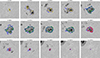 |
Fig. 8. Same as Fig. 6, but for sunspot NOAA AR 11381 (HARP 1210 dataset). |
| In the text | |
|
Fig. 9. Same as Fig. 5, but for sunspot NOAA AR 11084 (HARP 71 dataset). The sunspot remains stable over the full ≈200-hour interval, with ⟨B⟩ staying nearly constant at a value consistent with ⟨B⟩inv. |
| In the text | |
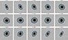 |
Fig. 10. Same as Fig. 6, but for sunspot NOAA AR 11084 (HARP 71 dataset). |
| In the text | |
Current usage metrics show cumulative count of Article Views (full-text article views including HTML views, PDF and ePub downloads, according to the available data) and Abstracts Views on Vision4Press platform.
Data correspond to usage on the plateform after 2015. The current usage metrics is available 48-96 hours after online publication and is updated daily on week days.
Initial download of the metrics may take a while.